Verification and Diagnosis Infrastructure of SoC HDL-model Vladimir Hahanov1, Wajeb Gharibi2, Eugenia Litvinova1, Svetlana Chumachenko1 1
Computer Engineering Faculty, Kharkov National University of Radioelectronics, Kharkov, Ukraine,
[email protected] 2 Jazan University, Jazan, Kingdom of Saudi Arabia,
[email protected]
Abstract — This article describes technology for diagnosing SoC HDL-models, based on transactional graph. Diagnosis method is focused to considerable decrease the time of fault detection and memory for storage of diagnosis matrix by means of forming ternary relations in the form of test, monitor, and functional component. The following problems are solved: creation of digital system model in the form of transaction graph and multi-tree of fault detection tables, as well as ternary matrices for activating functional components in tests, relative to the selected set of monitors; development of a method for analyzing the activation matrix to detect the faults with given depth and synthesizing logic functions for subsequent embedded hardware fault diagnosing. Keywords-system-on-chip; diagnosis; fault detection table; transaction graph, SoC HDL- model; infrastructure IP.
I.
TAB-MODEL FOR DIAGNOSIS FAULTY COMPONENTS OF SOC HDL-MODEL
Motivation of this paper is determined by the following: 1) the creation of simple and applicable models, methods and engines for diagnosis of multilayer software and hardware systems; 2) market appeal of matrix or table method for fault detection of SoC IP components (hardware and software) as the most effective one, which is focused on parallel processing and makes it possible to considerably reduce the time of faults diagnosis in non-functional mode. Aim of this article is creation of model and method for considerable decrease the testing time and memory for storage of diagnosis matrix by means of forming ternary relations (test – monitor – IP-function) in a single table TAB: Tests – Assertions – Blocks. The problems and background as published papers are: 1) development of diagnosability criteria and HDL digital system model in the form of transaction graph, as well as multi-level model and engine for diagnosis of software and hardware modules, based on activation matrix of functional components by using tests responded on the selected monitor set [1-6]; 2) development of a fault diagnosis method based on activation matrix analysis with a given depth [4-7]; 3) Implementation of diagnosis infrasructure in the system Riviera, Aldec [8-11].
Model for diagnosis of HDL digital system model is represented by the following transformation of the initial diagnosis equation, defined by xor-relation of the parameters : T F B 0 B T F B {T A} F , B {T A} {F m} which is transformed in ternary matrix relation of the T,F,B: M {{T A} {B}} Mij (T A)i B j . Here, the coordinate of matrix (table) is equal to 1, if the pair test–monitor (assertions) (T A)i activates faults of the functional block B j B on the monitors. A digital system model is presented as transaction graph: G B, A , B {B1, B2 ,...,Bi ,...,Bn }, , A {A1, A 2 ,...,A j ,...,A m } where sets of arcs B – functional blocks; A – monitors for observation of the HDL-code variables are defined. Test segments set T {T1, T2 ,...,Tr ,...,Tk } for HDLblocks diagnosis overlaps the graph model, and activates the transaction paths in the graph. In general, the testing model is represented by the Cartesian product M B A T that has the dimension Q n m k . To reduce the amount of diagnostic information it is offered to assign assertion monitor to each test segment, which answers for visualization of an activation way of functional blocks. It makes possible to decrease the dimension of model (matrix) to Q n k and retain all features of the triad relationship M B A T . For the pair «test – monitor» not only one-to-one correspondence is possible Ti A j , but functional
{Ti , Tr } A j
Ti {A j , As }
are
used
and too.
injective Such
variety
ones of
correspondences makes it possible to duplicate one test segment for different monitors, as well as assign several tests to the same monitor. At that the matrix cell Mij {0,1} always preserves its dimension, equal to 1 bit. The analytical matrix diagnosis model by using monitor engine, focused to achieving a given depth of faulty code diagnosis, is presented in the following form:
M f (G, L, T, B, A, t ), B {B1, B2 ,...,Bi ,...,Bm }; L {L1, L 2 ,...,Li ,...,L n }; A(t) {A1, A 2 ,...,A i ,...,A k }; A L; G L B; k n; T {T1, T2 ,...,Ti ,...,Tp }. Here Bi is a group of code statements, assigned to the node L i (variable, register, counter, memory), determining its state; G is functionality, presented by the transaction graph G (L, A) B in the form of the Cartesian product of node and arc sets; A is a set of monitors, as a subset of transaction graph nodes A L . The method for detecting faults of the functional blocks (FB) uses pre-built activation table (matrix) ATFB M [M ij] , where row is the relation between the test segment and a subset of activated blocks Ti A j (M i1, Mi2,...,Mij,...,Min ), Mij {0,1} , observed by the monitor A j . Column of the table describes the relation between the functional block, test segments and monitors M j B j f (T, A) . In the monitor engine the simulated time can be introduced, which complicates the activation matrix, and indicate real or simulated cycle, on which monitoring the node or functional block states on the test segment A j f (Ti , B j , t j ) is performed. At the modeling stage of fault diagnosis the response (column vector) m {m1, m2 ,...,mi ,...,mp } of monitor engine A on the test segments T is determined, by mi f (Ti , Ai ) . Searching faulty functional blocks is based on the definition of xor-operation between the assertion state vector and columns of the functional violation table m (M1 M 2 ... M j ... M n ) . The choice of solution is realized by using a method for xor-analysis columns, to choose a set of vectors B j with minimum number of unit coordinates: p
p
i 1
i 1
B min [B j (Bij mi )] , j1,n
forming the functional blocks with faults, verified on the test segments. In addition to the model for matrix diagnosis is necessary to describe the following important features of the matrix: 1) M i (Ti A j ); m
2) M ij M j 1; i 1
n
3) M ij M rj M ij; j1 k
4) M ij M ir M ij; i 1
5) log 2 n k log 2 B T 6) B j f(T, A) B T A 0. The features means: 1) Each row of the matrix is a match or subset of the Cartesian product (test – monitor).
2) Disjunction of all rows of the matrix gives a vector equal to one over all the coordinates. 3) All rows are distinct, which eliminates the test redundancy. 4) All columns of the matrix are distinct, which exclude the existence of equivalent faults. 5) The number of matrix rows must be greater than the binary logarithm of the columns number that determines the potential diagnosability of all blocks. 6) Diagnosis function for block depends on the complete test and monitors, which must be minimized without reduction the diagnosability. II.
DIAGNOSABILITY OF SOC HDL-MODEL
As for the model quality for diagnosis functional violations, it shows the efficiency of the use of pair (test, assertions) for a given diagnosis depth. Evaluation of the model quality is functionally dependent on the length of the test T , a assertions number A , and detected blocks number with functional violation N d on the total number of software blocks N: ]log 2 N[ N d . Q ED TA N The diagnosis efficiency is the ratio of the minimum number of bits needed for identification (recognition) of all the blocks to the real number of code bits, presented by the product of test length by number of assertions in each of them. If the first estimate fraction is equal to 1 and all the blocks with functional violation are detected ( Nd N ), it means a test and assertions are optimal that gives value of 1 for quality criterion of diagnosis model. Evaluation of the structure quality for the design code is interested as the perspective of the diagnosability of software blocks. The purpose of the analysis is determining the quantitative assessment of the graph structure and a node for placement of assertion monitors, which make possible to obtain maximum diagnosis depth of functional violation of the software components. It is important not controllability and observability as in testability, but the distinguish ability of the software components with functional violation, in the limit it is zero blocks with the equivalent (indistinguishable) violation. Such an assessment may be useful to compare the graphs implemented the same functionality. It is necessary to evaluate the graph structure from the position of potential detection depth of software functional violation. One possible option is diagnosability of ABC-graph as a function depending on adjacent arcs of each node (the number N n ), one of which is incoming, other one is outgoing. These arcs form paths without reconvergent fan-outs and branching (N is total number of arcs in the graph): N - Nn D . N Each node, joining two arcs entering in the number N n , is called transit one. The estimation N n is the number of indistinguishable functional violation of the software components. Potential locations of monitors for
distinguishing functional violation are transit nodes. Given the above estimation of the diagnosability D the diagnosis model quality for software takes the form: ]log 2 N[ N - N n . Q ED TA N Rules for synthesis of diagnosable software: 1) Test (testbench) must create minimum number of onedimensional activation paths, covered all the nodes and arcs of ABC-graph. 2) The base number of monitor-assertions equals the number of end nodes of the graph with not outgoing arcs. 3) An additional monitor can be placed in each node, which has one incoming and one outgoing arc. 4) Parallel independent code blocks have n monitors and a single test or one integrated monitor and n tests. 5) Serially connected blocks have one activation test for serial path and n-1 monitor or n tests and n monitors. 6) The graph nodes, which have different numbers of input and output arcs, create the conditions for the diagnosability of current section by one-dimensional activation tests without having to install additional monitors. 7) The set of test segments (testbench) has to be 100% functional coverage, given by the nodes of ABC-graph. 8) Diagnosability function is directly proportional to the test length, the number of assertions and inversely proportional to the binary logarithm of the number of software blocks: TA N - Nn D f (T, A, N) . N ]log 2 N[ Diagnosability as a function depending on the graph structure (for software), test and assertion monitors can always be reduced to unit value. For this purpose there are two alternative ways. The first one is increase of test segments, activating new paths for distinguishing equivalent faults without increasing assertions, if the software graph structure allows the potential links. The second is placement of additional assertion monitors in transit nodes of the graph. A third hybrid variant is possible, based on the joint application of two above ways. The relation of three components (the number of software blocks, the power of assertion engine and the test length) forms the set of optimal solutions TA D 1 1 ]log 2 N[ T A , ]log 2 N[ when quality of the diagnosis and diagnosability model is equal to 1. It can be useful for choosing an quasioptimal variant of alternative way for providing the full distinguish ability of software functional violation on a pair T A . III.
MODEL FOR DETECTING FUNCTIONAL FAILURES IN SOFTWARE
An analytic model for verification of HDL-code by using temporal assertion engine (additional observation lines) is focused to achievement the specified diagnosis depth and presented as follows:
M f (F, A, B, S, T, L), A {A1 , A 2 ,...,A i ,...,A n }; S {S1 , S 2 ,...,Si ,...,S m }; T {T1 , T2 ,...,Ti ,...,Tk };
F (A * B) S; S f (T, B); B {B1 , B 2 ,...,Bi ,...,B n }; Si {Si1 , Si2 ,...,Sij,...,Sip}; L {L1 , L 2 ,...,L i ,...,L n }.
Here F (A * B) S is functionality, represented by CodeFlow Transaction Graph – CFTG (Fig. 1); S {S1, S2 ,...,Si ,...,Sm} are nodes or states of software when simulating test segments. Otherwise the graph can be considered as ABC-graph – Assertion Based Coverage Graph. Each state Si {Si1, Si2,...,Sij,...,Sip} is determined by the values of design essential variables (Boolean, register variables, memory). The oriented graph arcs are represented by a set of software blocks n
n
i 1
i 1
B (B1, B2 ,...,Bi ,...,Bn ), Bi B; Bi , where the assertion Ai A {A1, A2 ,...,Ai ,...,An } can be put in correspondence to each of them. Each arc Bi – a sequence of code statements – determines the state of the node depending on the test Si f (T, Bi ) T {T1, T2 ,...,Ti ,...,Tk } . The assertion monitor, uniting the assertions of node incoming arcs A(Si ) Ai1 Ai2 ... Aij ... Ain can be put in correspondence to each node. A node can have more than one incoming (outcoming) arc. A set of functionally faulty blocks is represented by the list L {L1, L2 ,...,Li ,...,Ln } .
B (B1B3 B9 (B 2 B 7 B1B5 )B11)B13 (( B1B 4 B 2 B 6 )B10 B 2 B8 B12 )B14 B1B3 B9 B13 B 2 B 7 B11B13 B1B5 B11B13 B1B 4 B10B14 B 2 B 6 B10B14 B 2 B8 B12B14 . Figure 1. Example of ABC-graph for HDL-code
The model for HDL-code, represented in the form of ABC-graph, describes not only software structure, but test slices of the functional coverage, generated by using software blocks, incoming to the given node. The last one defines the relation between achieved on the test variable space and potential one, which forms the functional coverage p
as the power of state i-th graph node Q cardC ir / cardC i . In the aggregate all nodes have to be full coverage of the state space of software variables, which determines the test
m
m
i 1
i 1
quality, equal to 1 (100%): Q card Cir / card Cip 1 . Furthermore, the assertion engine A, C that exists in the graph allows monitoring arcs (code-coverage) A {A1, A2 ,...,Ai ,...,An } and nodes (functional coverage) C {C1, C2 ,...,Ci ,...,Cm} . The assertions on arcs are designed for diagnosis of the functional failures in software blocks. The assertions on graph nodes carry information about the quality of test (assertion) for their improvement or complement. The Code-Flow Transaction Graph makes possible the following: 1) use the testability design to estimate the software quality; 2) estimate the costs for creating tests, diagnosing and correcting the functional failures; 3) optimize test synthesis by means of solving the coverage problem by the minimum set of activated paths of all arcs (nodes). For instance, the minimum test for the above mentioned ABC-graph has six segments, which activate all existent paths:
T S0S1S3S7 S9 S0S1S 4S8S9 S0S1S5S7 S9 S0S 2S 4S8S9 S0S 2S5S7 S9 S0S 2S6S8S9 .
monitors (assertions or bits of boundary scan register) under all test patterns. If at least one coordinate of vector xor-sum rs is equal to zero Brs j A 0 then one of the following action is performed: the transition to the activation matrix of
lower level Brj 1,s or repair of the functional block B rs j . At that analysis is carried out, what is the most important: 1) time – then repair of faulty block is performed; 2) money – then a transition down is carried out to specify the fault location, because replacement of smaller block substantially decreases the repair cost. If at least one coordinate of the rs resulting xor-sum vector is equal to one Brs j A 1 , then transition to the next matrix column is performed. When all coordinates of the assertion monitor vector are equal to zero
A rs 0 , fault-free state of a device is fixed. If all vector rs sums are not equal to zero Brs j A 1 , it means a test, generated for check the given functionality, has to be corrected.
Tests can be associated with the following program block activization matrix: Bij B1 B2 B3 B4 B5 B6 B7 B8 B9 B10 B11 B12 B13 B14 T1 1 . 1 . . . . . 1 . . . 1 . T2 1 . . 1 . . . . . 1 . . . 1 T3 1 . . . 1 . . . . . 1 . 1 . T4 . 1 . . . 1 . . . 1 . . . 1 T5 . 1 . . . . 1 . . . 1 . 1 . T6 . 1 . . . . . 1 . . . 1 . 1
The activization matrix shows the fact of indistinguishability of the functional failures on a test in the blocks 3 and 9, 8 and 12, which constitute two equivalence classes if there is one assertion (monitor) in the node 9. To resolve this indistinguishability it is necessary to create two additional monitors in the nodes 3 and 6. As a result, three assertions in the nodes A (A3 , A6 , A9 ) allow distinguishing all the blocks of software code. Thus, the graph enables not only to synthesize the optimal test, but also to determine the minimum number of assertion monitors in the nodes to search faulty blocks with a given diagnosis depth. IV.
MULTILEVEL METHOD (ENGINE) FOR DIAGNOSIS OF DIGITAL SYSTEM
Process model or method for searching faults by diagnosis multi-tree is reduced to creation of the engine (Fig. 2) for traversal of tree branch on the depth, specified by the user: 0 {Br 1,s , R}; j rs rs Bj A rs 1 {B j1, , T}.
Here vector xor-operation is executed between the columns of the matrix and the output response vector A rs , which is determined by the functionality response taken from the
Figure 2. Engine for traversal of diagnosis multitree
Thus, the dataflow shown in the Fig. 2, allows realizing efficient infrastructure IP for complex technical systems. The advantages of the engine, which is invariant to the hierarchy levels, are the simplicity of preparation and presentation of diagnostic information in the form of minimizing activation table of functional blocks on the test patterns. V.
VERIFICATION OF MODELS AND METHOD FOR DIAGNOSIS
To illustrate the performance of the proposed model and method the functionalities of three modules of the digital filter of Daubechies [11] are considered below. The first component is component Row_buffer; its transaction graph, based on RTL-model, shown in Fig. 3. Nodes are presented by the states of variables and monitors, which are responsible for node incoming transactions or arcs, corresponding to the functional blocks.
Second test case for the practical use of the activation model and xor-method for searching faults is presented below. Synthesis of the diagnosis matrix for discrete cosine transform module from Xilinx library in the form of functional coverage is shown in Listing 1. Listing 1. Part of functional coverage Figure 3. Component Row_buffer of transaction graph
An activation table for functional blocks is generated by using graph, obtained during the simulation (Table I). Table rows are activation paths for blocks to the given monitornode. A table is a coverage all columns or functional blocks by rows of paths. In this case it should not have at least two identical columns. The difference of table is creation of the pair , making it possible to considerably reduce the dimension of the table with 100% detection of all faulty blocks. The main feature of the proposed model is the ability to describe the following relations by using the table: distinct tests – one node, one test – distinct nodes. TABLE I. A ij t1 D 3 t 2 D1 t 3 D1 t 4 D1 t 5 D1 t 6 D1 t 7 D2 t8 D2 t9 D2 t10 D 2 t11 D 2
T1 T2 . . 1 . . . . . . . . . . 1 . . . . . . . .
T3 . . 1 . . . . . . . .
T4 . . . . . . . 1 . . .
ACTIVATION TABLE T5 . . . 1 . . . . . . .
T6 . . . . . . . . 1 . .
T7 . . . . . . . . . 1 .
T8 1 . . . . . . . . . .
T9 . . . . . 1 . . . . .
T10 T11 T12 T13 . . . . . . . 1 . . . 1 . . . 1 . 1 . 1 . . . 1 . . 1 . . . 1 . . . 1 . . . 1 . 1 . 1 .
The use of the activation matrix of functional blocks (transaction graph) and xor-method for detecting faults allows synthesizing logic functions for the combination circuit, which determines number of functional block with semantic errors in process of simulation:
D3 T81 ; 1 1 1 1 1 1 1 1 1 1 D1 T13 T1 T13 T3 T13 T5 T13 T11 T13 T9 ; 1 1 1 1 1 1 1 1 1 1 D2 T12 T2 T12 T4 T12 T6 T12 T7 T12 T10 .
This feature is possible due to the lack of equivalent faults or identical columns in the activation matrix. Therefore, fixing the actual state of monitors at the nodes D1, D2 , D3 on 11 test patterns makes it possible to unambiguously identify an incorrect functional module by performing xor-operation between the assertion vector and the columns of activation matrix. Zero value of all coordinates for the result of xor-operations determines the number of the column corresponding to a faulty module. The implementation of the model and method in a logical function allows identifying the faulty block before the completion of the diagnosing experiment, if it is possible. This means significant savings of diagnosis time for certain types of faults. For instance, the test-monitor t1 D3 allows identifying a fault of the block B8 at the first test.
c0: coverpoint xin { bins minus_big={[128:235]}; bins minus_sm={[236:255]}; bins plus_big={[21:127]}; bins plus_sm={[1:20]}; bins zero={0}; } c1: coverpoint dct_2d { bins minus_big={[128:235]}; bins minus_sm={[236:255]}; bins plus_big={[21:127]}; bins plus_sm={[1:20]}; bins zero={0}; bins zero2=(0=>0); } endgroup
For all 12 modules the transaction graphs, activation tables, and logic functions are developed for testing and fault detection in the discrete cosine transform. Graph with the activation matrix and logic function (Fig. 4) are presented below. This graph is associated with the following diagnosis matrix (Table II). TABLE II.
DIAGNOSIS MATRIX
A ij T1 T2 T3 T4 T5 T6 T7 T8 T9 T10 T11 T12 T13 T14 P1 F7 1 . 1 . 1 . 1 . . . . . . . P2 F8 . 1 . 1 1 . . 1 . . . . . . P3 F9 1 . 1 . . 1 . . . . 1 . . . P4 F10 . 1 . 1 . 1 . . . . . 1 . . P5 F12 1 . 1 . 1 . . . 1 . . . 1 . P6 F13 . 1 . 1 . 1 . . . 1 . . . 1 P1 F2 1 . . . . . . . . . . . . . P2 F3 . 1 . . . . . . . . . . . .
The system of diagnosis functions is presented below: 1 1 1 1 F7 T11T31T51T71 ; F8 T21T41T51T81 ; F9 T11 T6T1 T3 ; 1 1 F10 T41T51T61T12 ; F12 T11T31T51T91T13 ; 1 1 F13 T21T41T61T10 T14 ;
F2 T11 ; F3 T21 ; Fragment of monitor engine is presented by Listing 2. Listing 2. Code fragment of monitor engine sequence first( reg[7:0] a, reg[7:0]b); reg[7:0] d; (!RST,d=a) ##7 (b==d); endsequence property f(a,b); @(posedge CLK) // disable iff(RST||$isunknown(a)) first(a,b); !RST |=> first(a,b); endproperty
odin:assert property (f(xin,xa7_in)) // $display("Very good"); else $error("The end, xin =%b,xa7_in=%b", $past(xin, 7),xa7_in);
Figure 5. Implementation of results in the system Riviera Time-to-market comparison Time-to-market (KMen/Hour)
30,00 25,00 20,00
Design + Classic Testbench Design + Stimulus + Assertions
15,00 10,00 5,00 0,00 0,112 0,207 0,315 0,389 0,504 0,620 0,731 0,824 0,931 1,015
Design capacity (MGates)
Figure 4. Transaction graph of main-RTL module
Testing of discrete cosine transformation in the environment Riviera, Aldec detects incorrectness in seven rows of HDL-models: //add_sub1a