Verification and Validation and Artificial Intelligence Tim Menzies Computer Science, Portland State University, Oregon, USA
Charles Pecheur RIACS at NASA Ames Research Center, Moffett Field, CA, USA
Abstract Artifical Intelligence (AI) is useful. AI can deliver more functionality for reduced cost. AI should be used more widely but won’t be unless developers can trust adapative, nondeterministic, or complex AI systems. Verification and validation is one method used by software analysts to gain that trust. AI systems have features that make them hard to check using conventional V&V methods. Nevertheless, as we show in this article, there are enough alternative readily-available methods that enable the V&V of AI software.
1
Introduction
Artificial Intelligence (AI) is no longer some bleeding technology that is hyped by its proponents and mistrusted by the mainstream. In the 21st century, AI is not necessarily amazing. Rather, it is often routine. Evidence for the routine and dependable nature of AI technology is everywhere (see the list of applications in [1]). AI approach has always been at the forefront of computer science research. Many hard tasks were first tackled and solved by AI researchers before they Email addresses:
[email protected] (Tim Menzies),
[email protected] (Charles Pecheur). URLs: http://menzies.us (Tim Menzies), http://ase.arc.nasa.gov/pecheur (Charles Pecheur).
Preprint submitted to Elsevier Science
12 July 2004
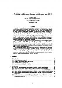
transitioned to standard practice. Those examples include time-sharing operating systems, automatic garbage collection, distributed processing, automatic programming, agent systems, reflective programming and object-oriented programming. This tradition of AI leading the charge and solving the hard problems continues to this day. AI offers improved capabilities at a reduced operational cost. For example, Figure 1 describes the AI used in NASA’s Remote Agent Experiment (RAX) [2]. For over a day, this system ran a deep-space probe without any help from mission control. Such AI-based autonomy is essential to future deep space missions. NASA needs such autonomous software so that deep space probes can handle unexpected or important events billions of miles away from earth when they are hours away from assistance by mission control. AI software can be complex and the benefits of complexity are clear. Some applications such as the RAX described in Figure 1 are inherently complex and require an extension to existing technology. However, the cost of complexity is that complex systems are harder to understand and hence harder to test. Complex systems like can hide intricate interactions which, if they happen during flight, could compromise the mission. For example, despite a year of extensive testing, when Remote Agent was first put in control of NASA’s Deep Space One mission, it froze because of a software deadlock problem (RAX was re-activated two days later and successfully completed all its mission objectives). After analysis, it turns out that the deadlock was caused by a highly unlikely race condition between two concurrent threads inside Remote Agent’s executive. The scheduling conditions that caused the problem to manifest never happened during testing but indeed showed up in flight [2]. Hardware engineers solve such problems with hardware redundancy (when one component fails, its back-up wakes up and takes over). However, redundancy may not solve software reliability problems. Hardware components fail statistically because of wear or external damage. Software components programs fail almost exclusively due to latent design errors. Failure of an active system is thus highly correlated with failure of a duplicate back-up system (unless the systems use different software designs, as in the Space Shuttle’s on-board computers). If redundancy may not increase the reliability of AI software, what else should we do to check our AI software? How should standard verification and validation (V&V) be modified to handle AI systems? What are the traps of V&V of AI software? What leverage for V&V can be gained from the nature of AI software? This article offers an overview of the six features of AI systems that a V&V analysts must understand. An AI system may be: 2
NASA’s deep space missions require autonomous spacecrafts that don’t rely on ground control. The Remote Agent Experiment (RAX) was an experiment in autonomy technology: for two days, RAX provided on-board AI control for the Deep Space One probe, while it was 60,000,000 miles from Earth. RAX had three main components. The Planner & Scheduler (PS) took general goals and determined detailed activities needed to achieve the goals. If a hardware problem developed that prevents execution of the plan, the planner made a new plan, taking into account degraded capabilities. The Smart Executive (EXEC) interpreted the plans and added more detail to them, then issued commands to rest of the satellite. Lastly, the Mode Identification and Recovery (MIR) component (based on the Livingstone diagnosis system) acted like a doctor, monitoring the spacecraft’s health. If something went wrong, MIR would detect it and report it to EXEC. Exec could then consult the “doctor” for simple procedures that may quickly remedy the problem. If those simple procedures could not resolve the problem, EXEC asked PS for a new plan that still achieved the mission goals while accounting for the degraded capabilities. Fig. 1. The Remote Agent Experiment, from http://cmex-www.arc.nasa.gov/CMEX/RemoteAgent.html
3
(1) complex software; (2) declarative and model-based, and sometimes knowledge-level software; (3) nondeterministic or even adaptive software. Fortunately, not all AI systems have all the above features since each can come with a significant cost. However, each of these features grants significant benefits that can make the costs acceptable. The rest of this article is structured around this list of features of an AI system. Each feature will be defined and their associated cost and benefits will be discussed. To help the reader who is a not an AI specialist, many of our sections start with short tutorials. Note that the approach of this review is different to the traditional reviews of AI verification (e.g. [3–15]) or AI (e.g. [16–24]). Much has changed since the early days of AI and the field has moved on to more than just simple rule-based systems. While other articles offer success stories with that representation (e.g. [25–28] and Chapt. 8,30,31,34 in [29]), this review focuses on the features of modern AI that distinguishes it from conventional procedural software; e.g. nondeterministic adaptive knowledge-level systems. If the reader is interested in that traditional view, then they might care to read the references in this paragraph (in particular [4, 24, 28, 29]) or one of the many excellent on-line bibliographies on V&V of AI systems 1 .
2
AI Software can be Complex
The rest of this paper stresses what is different about AI systems and how those differences effect V&V for AI. Before moving on to that material, this section observes that AI software is still software, albeit sometimes quite complex software. Hence, methods developed for assessing normal software systems still apply to AI systems. V&V analysts should view this article as techniques that augment, not replace their standard V&V methods such as peer reviews, automated test suites, etc [30–32]. In this section, we review the state-of-the-art in verifying complex software. Many of these techniques are routinely applied at NASA when verifying complex AI systems such as RAX. We start with conventional testing as a baseline, then introduce more advanced formal methods: run-time monitoring, static analysis, model checking and theorem proving. Those methods vary in the strength of the verdicts they provide, as well as the level of expertise they require—generally speaking, 1
e.g. http://www.csd.abdn.ac.uk/~apreece/Research/vvbiblio.html
4
Expertise Testing
Run-Time Static Monitoring Analysis
Theorem Model Checking Proving
Strength
Fig. 2. The verification methods spectrum.
more thorough approaches require more expertise. This can be laid out as the “verification methods spectrum” shown in Figure 2 2 .
2.1
Testing
Traditionally, software verification is done using scenario-based testing. The system to be verified is embedded into a test harness that connects to the inputs and outputs of that component, and drives it through a suite of test runs. Each test run is an alternated sequence of provided inputs and expected outputs, corresponding to one scenario of execution of the tested component. An error is signaled when the received output does not meet the expected one. Even for simple systems, the design and maintenance of test suites is a difficult and expensive process. It requires a good understanding of the system to be tested, to ensure that a maximum number of different situations are covered using a minimum number of test cases. Running the tests is also a timeconsuming task, because the whole program code has to be executed and everything must be re-initialized before each test run. In the development of complex systems, it is quite common that testing the software actually takes more resources than developing it. While traditional testing may be enough for more conventional software, it falls short for complex AI software, mainly because the range of situations to be tested is incomparably larger. A typical intelligent program implicitly incorporates responses to a very large space of possible inputs (for example, consider the possible interaction sequences that an autonomous agent like RAX may face). The internal state of the program is typically huge, dynam2
Adapted from John Rushby, in slides of [33]. This spectrum is notional and expresses trends rather than absolute truths. In particular, a comparative experimental evaluation conducted at NASA [34] concluded that static analysis may require a deep understanding of its underlying algorithms to be used effectively.
5
ically allocated (heap memory, garbage collection) and may involve complex data structures (knowledge, rules, theories). It depends on the past history of the system in intricate ways. AI systems may involve several concurrent components, or other sources of non-determinism. Because of all these factors, a test suite can only exercise a very limited portion of the possible configurations, and it is very hard to assess how much has been covered and therefore measure the residual risk of errors.
2.2
Run-Time Monitoring
Run-time monitoring, or run-time verification, refers to advanced techniques for scrutinizing artifacts from an executing program (variables, events, typically made available through program instrumentation), in order to detect effective or potential misbehaviors or other useful information. Simple runtime monitoring methods have been used for decades. For example, it is standard practice for programmers to add conditionals to their code that print warning messages if some error condition is satisfied, or to generate and scan additional logging messages for debugging purposes. In essence, runtime verification automates the otherwise strenuous and error-prone task of reviewing these logs manually. This analysis can be conducted after-the-fact on stored execution traces, but also on-the-fly while the program is executing. In this latter case, the need to store the execution trace is alleviated, and the monitor can also trigger recovery mechanisms as part of a software fault protection scheme. Recently, the sophistication of runtime monitoring methods has dramatically increased. Commercial tools such as Temporal Rover [35] can instrument a program to execute inserted code fragments based on complex conditions expressed as temporal logic formulae (see Figure 3). New algorithms can detect suspicious concurrent programming patterns (data races [36], deadlocks [37]) that are likely to cause an error, even if no error occurs on the observed trace. Runtime monitoring typically requires little computing resources and therefore scales up well to very large systems. On the other hand, it will only observe a limited number of executions and thus gives only uncertain results. In the case of error predictions, it can also give false negatives, i.e. flag potential errors that cannot actually occur. One example of a runtime monitoring system is Java Path Explorer (JPaX) [37]. Given a specification of properties to be monitored, JPaX instruments a Java program to generate a trace of relevant events. JPaX also produces an 6
A temporal logic is a classical logic augmented with operators to reason about the evolution of the model over time. Temporal logic allows to express conditions over time, such as “any request is always eventually fulfilled”. For example, (propositional) linear temporal logic, or LTL uses the following operators: Property
Reads
Means p holds . . .
◦p
“next p”
2p
“henceforth p”
. . . in all future states
3p
“eventually p”
. . . in some future state
pUq
“p until q”
. . . in the next state
. . . in all states until q holds
Fig. 3. About temporal logic.
observer program that reads that trace and verifies the properties. The trace can be streamed through a socket, to allow local or remote on-the-fly monitoring. Both user-provided temporal logic conditions and generic deadlock and data race conditions can be monitored. In [38], run-time monitoring is applied (in conjunction with automated testcase generation) to verify the controller of the K9 planetary rover. The controller is a large multi-threaded program (35,000 lines of C++) that controls the rover according to a flexible plan generated by a planning program. Each test case amounts to a plan, for which a set of temporal properties are derived, according to the semantics of the plan. The EAGLE system [39] is then used to monitor this properties. This system is fully automated and unveiled a flaw in plan interpretation, that indeed occurred during field tests before it was fixed in the controller. A potential deadlock and a data race were also uncovered.
2.3
Static Analysis
Static Analysis consists in exploring the structure of the source code of a program without executing it. It is an important aspect of compiler technology, supporting type analysis and compiler optimizations. A good reference textbook on the topic can be found in [40]. Static analysis includes such aspects as control- and data-flow analysis (tracking the flows of execution and the propagation of data in the code), abstract interpretation (computing abstract approximations of the allowed ranges of program variables) and program slicing (capturing the code portions that are relevant to a particular set of variables or a function). In principle, static analysis can be applied to source code early in the devel7
Fig. 4. Slicing in Grammatech’s CodeSurfer tool http://www.grammatech.com/products/codesurfer/example.html).
(see
opment and is totally automatic. There is, however, a trade-off between the cost and the precision of the analysis, as the most precise algorithms have a prohibitive complexity. More efficient algorithms make approximations that can result in a large number of false positives, i.e. spurious error or warning messages. Two commercial static analysis tools are Grammatech’s CodeSurfer and the PolySpace Verifier [41]. Figure 4 shows CodeSurfer using a static control flow analysis to find the code not reachable from the main function. Such code is dead code and represents either over-specification (i.e. analysts exploring too many special cases) or code defects (e.g. the wrong items are present in a conditional). In Figure 4 the code sections reached from main are shown with dark colored marks in the right-hand-side of the display. Note that in this case, most of the code is not reachable from the main program. PolySpace uses abstract interpretation to find potential run-time errors in (C or Ada) programs such as: • • • • • •
access to non-initialized variables, unprotected shared variables in concurrent programs, invalid pointer references, array bound errors, illegal type conversions, arithmetic errors (overflow, underflow, division by zero, . . . ), 8
• unreachable code. The output of the tool consists of a color-coded version of the program source code, as shown on Figure 5. Green code is guaranteed free from errors, red code is sure to cause errors, orange code may cause errors (depending on execution paths or because the analysis was inconclusive), and grey code is unreachable.
green (ok)
red (error)
orange (warning) grey (unreachable)
Fig. 5. An example of color-coded source code produced by the PolySpace Verifier. From http://www.polyspace.com/datasheets/c_psde.htm (callouts added).
Once the code to be analyzed has been identified, static analysis tools such as CodeSurfer and PolySpace are fully automatic. However, the experiment reported in [34] concludes that their use can be a labor-intensive, highly iterative process, in order to: (i) isolate a proper self-standing code set to be analyzed, (ii) understand and fix the reported red errors, (iii) adjust analysis parameters to reduce the number of false alarms. The last point can be very detrimental, as the analysis tends to return a very large number of mostly spurious “orange” warnings, making it very hard to identify real errors. The C Global Surveyor tool (CGS), currently under development at NASA, drastically reduces this problem by specializing the analysis algorithms to the coding practices of a specific class of applications [42]. 9
2.4
Model Checking
Model Checking consists in verifying that a system (or a model thereof) satisfies a property by exhaustively exploring all its reachable states. Model checking was invented in the 1980s to analyze communication protocols [43,44], and is now routinely employed in verification of digital hardware. Several mature and powerful model checkers are available and widely used in the research community; SPIN [45] and SMV [46,47] are probably the best known. See [48] for a comprehensive theoretical presentation, and [49] for a more practical introduction. A model checker searches all pathways of the system looking for ways to violate the property. This requires that this state space be finite and tractable: model checking is limited by the state space explosion problem, where the number of states can grow exponentially with the size of the system. 3 Tractability is generally achieved by abstracting away from irrelevant details of the system. If a violation is found, the model checker returns the counter examples showing exactly how the property is violated. Such counter examples are useful in localizing and repairing the source of the violation. Model checking requires the construction of two models: • The systems model is an abstract description of the dynamic, generally concurrent behavior of a program or system. For tractability reasons, it is usually not the complete code from the implementation but rather some abstract verification model of the application, capturing only the essential features that are relevant to the properties to be checked. • The properties model is a specification of the requirements that should hold across the systems model. The properties model is often expressed as a temporal logic constraint. 4 Model checkers often impose their own modeling language for both the systems and the properties, though more and more tools now apply directly to common design and programming languages (UML, Java), either natively or through translation. 3
When the state space is too large or even infinite, model checking can still be applied: it will not be able to prove that a property is satisfied, but can still be a very powerful error-finding tool. 4 Depending on the model checker being used, properties are sometimes expressed in other forms, such as invariants that must hold in every state, regular expressions that execution traces must match, or other dynamic system models whose executions must agree (in some precisely defined sense) with those of the verified system (see e.g. [50]).
10
Although model checkers are automatic tools, the benefits of model checking come at a cost that is often very significant. That cost can be divided into three components: • writing cost: the initial cost of developing the systems model and the properties model, in a form accepted by the model checker; • running cost: the cost of actually performing the model checking, as many times as necessary; and • re-writing cost: the cost of iteratively modifying the models until model checking can complete successfully and provide acceptable results. With traditional model checking tools, both the systems model and the properties model have to be written in their own tool-specific language, which often results in high writing cost. In particular, scarce and expensive PhDlevel mathematical expertise may be required to properly encode properties in formal temporal logic. Once models have been completed, the model checker explores all the interactions within the program. In the worst case, the number of such interactions is exponential on the number of different assignments to variables in the system. Hence, the running cost of this query can be excessive. This large running cost generally forces analysts to simplify the formal models, for example by removing parts or functions, abstracting away some details, or restricting the scope of the analysis. Such a rewrite incurs the rewrite cost. On the other hand, simplification may take away elements that are relevant to the properties being verified, so a balance must be found between tractability and accuracy of the analysis. This typically requires several iterations and a significant amount of expertise in both the tools and the application being verified. Much research has tried to reduce these costs. The writing of systems models can be avoided by applying model checkers directly to readily available representations, such as design models or program code. For example, the BANDERA system extracts systems models from JAVA source code and feeds them into SMV or SPIN machine [51]. Java PathFinder applies model checking directly to Java bytecode, using its own custom Java virtual machine [52]. Other approaches such as SCR [53–55] or simple influence diagrams [56] propose simplified modeling environments where users can express their models in a simple and intuitive framework, and then map them into model checkers such as SPIN. Interestingly enough, AI software can offer good opportunities for model checking, as a consequence of using model-based or knowledge-based approaches. This aspect is discussed in detail in Section 3; for now let us point out that the models that are interpreted in AI systems tend to be abstract enough to be readily amenable to model checking, with only minor adaptation writing costs. 11
Pecheur and Simmons’ verification of models used for autonomous diagnosis using the SMV synbolic model checker is a good example [57]. On the properties side, Dwyer, Avrunin & Corbett [58, 59] have developed a taxonomy of temporal logic patterns that covers most of the properties observed in real-world applications. For each pattern, they have defined an expansion from the intuitive pseudo-English form of the pattern to a formal temporal logic formula. 5 These patterns are simpler and more intuitive than their logical counterpart, and shield the analysts away from the complexity of formal logics. For example, consider the following property on an elevator: Always, the elevator door never opens more than twice between the source floor and the destination floor. If P is the elevator doors opening and Q is the arrival at the source floor and R arrival at the destination floor, then the temporal logic formula for this property is: 2((Q ∧ 3R) → ((¬P ∧ ¬R) U (R ∨ ((P ∧ ¬R) U (R ∨ ((¬P ∧ ¬R) U (R ∨ ((P ∧ ¬R) U (R ∨ (¬P ∨ R)))))))))) In contrast, this property can be expressed using the “bounded existence” temporal logic pattern as “transitions to P -states occur at most 2 times between Q and R”, and then be automatically translated to the form above. The translator in [57] offers a similar facility, though focused on more specific property classes. These tools reduce the writing cost but don’t necessary reduce the running cost or the rewriting cost. The rewriting cost is incurred only when the running cost is too high and the models or constraints must be abbreviated. There is no guarantee that model checking is tractable over the constraints and models built quickly using temporal logic patterns and tools like SCR. Restricted modeling languages may generate models simple enough to be explored with model checking-like approaches, but the restrictions on the language can be excessive. For example, checking temporal properties within simple influence diagrams can take merely linear time [56], but such a language can’t model common constructs such sequences of actions or recursion. Hence, analysts may be forced back to using more general model checking languages. Despite decades of work and ever-increasing computing power, the high running cost of such general model checking remains a major challenge. Different 5
Actually, to several logic variants, including Linear Temporal Logic (LTL), Computation Tree Logic (CTL), Graphical Interval Logic (GIL), Quantified Regular Expressions (QRE) and INCA Queries.
12
techniques have proven to be useful in reducing the running cost of model checking: • Symbolic Methods represent and process parts of the state symbolically to avoid enumerating each individual value that they can take. This can be done at the level of individual model variables [60] or over the model as a whole, using boolean encodings such as binary decision diagrams [46] or propositional satisfiability solvers [61]. • Abstraction can be applied in a principled way to map large or infinite concrete spaces into small abstract domains. data abstraction applies to individual variables (e.g. abstracting an integer to its sign) [62], while predicate abstraction uses the values of predicates obtained from the model [63]. In either case, the abstraction is usually not exact and produces spurious traces (i.e. for which no concrete trace exists in the original model). • Partial Order Reduction analyzes dependency between concurrent operations to avoid exploring multiple equivalent permutations of independent operations. This is further discussed in Section 5.3. • Symmetry Reduction uses symmetry in the system (e.g. identical agents) to avoid exploring multiple symmetrical states or paths [64, 65]. • Compositional Reasoning divides the systems model into separate components, which can be reasoned about separately [66–68]. This generally involves some form of assume/guarantee reasoning, to capture the interdependency between the different components. • Model Reduction replaces the systems model by a reduced, simpler model that is equivalent with respect to the property being verified. For example, the BANDERA system [51] can automatically extract (slice) the minimum portions of a JAVA program’s byte codes which are relevant to particular properties models. While the above techniques have all been useful in their test domains, not all of them are universally applicable. Certain optimizations require expensive pre-processing, or rely on certain features of the system being studied. Not all systems exhibit reducible symmetry or concurrency that is amenable to partial order reduction. Compositional analysis is hard for tightly connected models. In the general case, model checking techniques are still limited to models of modest size, and obtaining these models from real applications requires significant work and expertise. Despite these limitations, model checking is a widely used tool for AI systems at institutions like NASA. For example, in 1997, a team at NASA Ames used the Spin model checker to verify parts of the RAX Executive and found five concurrency bugs [69]. Although it took less than a week to carry out the verification activities, it took about 1.5 work-months to manually construct a model that could be run by Spin in a reasonable length of time, starting from the Lisp code of the executive. The errors found were acknowledged and fixed 13
by the developers of the executive. As it turns out, the deadlock that occurred during the in-flight experiment in 1999 was caused by an improper synchronization in another part of the Executive, but was exactly of the same nature as one of the five bugs detected with Spin two years before. This demonstrates how this kind of concurrency bug can indeed pass through heavy test screens and compromise a mission, but can be found using more advanced techniques such as model checking. In the same vein, compositional verification has been applied to the K9 Rover executive [70]. Further examples can be found in the Proceedings of the recent AAAI 2001 Spring Symposium on Model-Based Validation of Intelligence 6 .
2.5
Theorem Proving
Theorem provers build a computer-supported proof of the requirement by logical induction over the structure of the program. In principle, theorem provers can use the full power of mathematical logic to analyze and prove properties of any design in its full generality. For example, the PVS system [71] has been applied to many NASA applications (e.g. [72]). However, these provers require a lot of efforts and skills from their users to drive the proof, making them suitable for analysis of small-scale designs by verification experts only. In contrast, the other methods discussed in the previous sections are largely automated, and thus more convenient for verification as part of a software development process. For this reason, theorem proving is still mostly limited to a few academic studies and regarded as inapplicable in an industrial setting. This view may change, however, as proof systems feature increasingly powerful proof strategies, that can automatically reduce most of the simpler proof obligations. Also note that recent developments in formal verification are blurring this distinction between proof-based and state-based approaches: on one side, proof systems are extended with model checkers that can be used as decision procedures inside larger proofs [73]; on the other side, novel symbolic model checking approaches use proof-based solvers to prune out impossible paths in the symbolic state space [60, 74].
3
Model-based AI Systems
Having discussed how V&V AI can leverage techniques developed for software engineering problems, we now turn to the special features of AI that change the V&V task. This section discusses model-based. Subsequent sections will discuss 6
http://ase.arc.nasa.gov/mvi/
14
knowledge-level systems, nondeterminism, adapation, and their implications for V&V. Every V&V analyst knows that reading and understanding code is much harder than reading and understanding high-level descriptions of a system. For example, before reading the “C” code, an analyst might first study some high-level design documents. The problem with conventional software is that there is no guarantee that the high-level description actually corresponds to the low-level details of the system. For example, after the high-level block diagram is designed, a programmer might add a call between blocks and forget to update the high-level block diagram. This disconnect between the specification and the implementation raises significant issues for formal verification. Often, formal verification techniques based on model checking (as opposed to those based on proof systems 7 ) are able to efficiently check all possible execution traces of a software system in a fully automatic way. However, the system typically has to be manually converted beforehand into the syntax accepted by the model checker. This is a tedious and complex process, that requires a good knowledge of the model checker, and is therefore usually carried externally by a formal methods expert, rather than by the system designer themselves. A distinct advantage of model-based AI systems is that the high-level description is the system. A common technique used in AI is to define a specialized, succinct, high-level modeling language for some domain. This high-level language is then used to model the domain. If another automatic tool is used to directly execute that notation, then we can guarantee that the high-level model has a correspondence to the low-level execution details 8 . These models are often declarative and V&V analysts can exploit such declarative knowledge for their analysis.
3.1
About Declarative Knowledge
Declarative representations can best be understood by comparing them to procedural representations used in standard procedural languages such as “C”. Procedural representations list the ordering of activities require to complete 7
Which can provide even more general results but require an even more involved and skilled guidance. 8 This article defines the term “model” in its most common usage; i.e. the thing that is generated by analysts when they record information about their domain. Logic programming theorists prefer the term “theory”. In logic, a “model” is some instance of a “theory” and is generated automatically at runtime.
15
some task. Procedural knowledge often manifests itself in the doing of something and may be hard to share with others except in the specific context where the procedural knowledge was developed. V&V analysts know how hard it can be to un-tangle procedural knowledge such as a “C” program. Declarative knowledge describes facts and relationships within a domain. Declarative knowledge can be easier to understand than procedural knowledge; it can be easier to modify, easier to communicate to others, and easier to reuse for different purposes. While procedural knowledge is about how, declarative knowledge is often statements about what is true in a domain. For example, consider the following piece of procedural knowledge. This implementation reports that you have “X” if it finds any evidence for any of the sub-types of “X”. Note that this is knowledge about how to navigate a hierarchy of diseases, and their symptoms. if ((record.disease(X)==found) && (diseases = record.disease(X).subtypes) ) for(disease in diseases) for(symptom in disease.symptoms) for (observation in observations) if symptom == observation printf("You have %s which is a type of %s!", disease, X); return 1
Suppose we wanted to report the disease that we have the most evidence for; i.e. the disease that has the most symptoms amongst the available observations. In this procedural representation, this change would imply extensive modification to the code. An alternate approach would be to use declarative representations that queried the following facts: subtype(bacterial, subtype(injury, subtype(bacterial, symptom(gastro, symptom(carAccident,
measles). carAccident). gastro). dehydration). wounds).
symptom(measles, symptom(measles, symptom(gastro,
temperature). spots). temperature).
Declarative representations free the analyst from specifying tedious procedural details. For example, the core logic of the above procedural code is that we have evidence for a disease is we have any observations consistent with subtyes of that disease. This can be expressed directly and declaratively as follows: %comments start with a percent sign evidence(Disease,SubType,Evidence):- % we have evidence if.. subtype(Disease,SubType), % we can find a subtype AND symptom(SubType,Evidence), % AND that subtype has symptoms observation(Evidence). % AND we can observe those symptoms
This declarative representation is useless without some interpreter that can exercise it. Our example here uses the syntax of the Prolog logic programming language [75]. In that language, upper case words are variables and lower case words are constants. 16
The major disadvantage of procedural knowledge is that it can be opaque and inflexible. Declarative knowledge, on the other hand, is far more flexible since the knowledge of what is separated from the how, This means that the what can be used in many ways. For example, suppose we want to drive the diagnosis backwards and find what might cause spots. To do this, we first must fool Prolog into believing that all observations are possible. Since we are using declarative representations, this is simple to do: we just make an “anything goes” assertion: observation(_).
Here, the “ ” is an anonymous variable that matches anything at all. In the language of Prolog, this means that we will assume any observation at all. With this “anything goes” in place, we can now drive the evidence rule backwards to find that spots can be explained via a bacterial infection. ?- evidence(Disease,SubType,spots). Disease = bacterial SubType = measles
A more complicated query might be to find evidence that disproves some current hypothesis. For example, suppose we believe the last query; i.e. the observed spots can be explained via a bacterial infection. Before we commence treatment, however, it might be wise to first check for evidence of other diseases that share some of the evidence for measles. Since our knowledge is declarative, we need not change any of the above evidence rule. Instead, we just reuse it in a special way: differentialDiagnosis(Disease,Old,Since,New,If) :evidence(Disease,Old,Since), evidence(Disease,New,Since), % Old and New share some evidence evidence(Disease,New,If), not evidence(Disease,Old,If). % New has some evidence not seen in Old
With this in place, we can run the following query to learn that measles can be distinguished from gastro if dehydration can be detected: ?- differentialDiagnosis(bacterial,Old,Since,New,If). Old Since New If
= = = =
measles temperature gastro dehydration
While the declarative version of knowledge might be faster to write and change, it may be slower to run. Procedural knowledge can be highly optimized to take advantage of low-level details of a system. In the 1970s, this was taken to be a major disadvantage of declarative knowledge. In the 21st century, this is much less of an issue. Not only are computers much faster now, but so are the interpreters for our declarative systems (e.g. [76, 77]), particularly when the 17
Livingstone
MPL Model
MPL Specification
MPL Trace
T R A N S L A T O R
SMV Model
SMV Specification
SMV
SMV Trace
Fig. 6. Translator from Livingstone to SMV (MPL is Livingstone’s modeling language).
representation can be restricted to some subset of full logic (e.g. [78, 79]).
3.2
Declarative Models and V&V
The ability to build simple queries for a declarative model greatly reduces the effort required for V&V. For example, one method for V&V of model-based systems is to build a profile of an average model. The TEIREISIAS [80] rule editor applied a clustering analysis to its models to determine what parameters where related; i.e. are often mentioned together. If proposed rules referred to a parameter, but not its related parameters, then TEIREISIAS would point out a possible error. Declarative modeling tend to only use a small number of modeling constructs. This simplifies the construction of translators from one modeling language to another, and in particular from AI modeling languages to verification modeling languages such as those used by model checkers (as discussed in §2.4). Moreover, the reasoning algorithms used in AI typically suffer from similarly high complexity metrics as model checking, and therefore the size and complexity of AI models is already limited by the scalability of their intended usage. Indeed, AI fields such as planning and scheduling have much in common with model checking, in the way they both explore a state space described by a model. This similarity has lead to some cross-fertilization between the two fields in the recent years, with verification adopting search heuristics from planning on one hand [81] and planners based on verification technology such as BDDs on the other hand [82]. For example, Pecheur and Simmons have developed a translator to convert Livingstone models to SMV [57]. Livingstone is a model-based health monitoring system developed at NASA [83]. It tracks the commands issued to the device and monitors device sensors to detect and diagnose failures. To achieve this, Livingstone relies on a model of the device that describes, for each component, the nominal and abnormal functioning modes, how these modes are affected by commands and how they affect sensors. The translator enables exhaustive analysis of those models using the powerful SMV model checker. 18
The essence of the translation is fairly straightforward, thanks to the similar semantics framework used in both Livingstone and SMV. The translator also supports user-oriented specification patterns and variables to express common classes of properties such as consistency or existence of a broken component. These declarations are captured and converted into the core temporal logic syntax accepted by SMV. Finally, the execution traces returned by SMV can be converted back into Livingstone syntax. Together, these three translation capabilities (model, properties, trace) isolate the Livingstone application developer from the peculiarities of SMV and provide the functional equivalent of a symbolic model checker for Livingstone, as depicted if Figure 6. The translator has been used at NASA Kennedy Space Center by the developers of a Livingstone model for the In-Situ Propellant Production (ISPP), a system that will produce spacecraft propellant using the atmosphere of Mars [84]. The latest version of the ISPP model, with 1050 states, could still be processed in less than a minute using SMV optimizations (re-ordering of variables). The Livingstone model of ISPP features a huge state space but little depth (all states can be reached within at most three transitions), for which the symbolic processing of SMV is very appropriate. This tool can be used to check general sanity properties (e.g. consistency, absence of ambiguity, no conflicting transitions) or specific expected properties of the modeled device (e.g. flow conservation, functional dependency between variables). More recently, the technique has been extended to verify diagnosability properties, i.e. the possibility for an ideal diagnosis system to infer accurate and sufficient information on the state of the device from its observed behavior [85]. Diagnosability amounts to the absence of certain pair of traces with identical observations, which can be turned into a simple model checking problem over a duplicated version of the original model. Model checking is powerful, but can be complicated. Feather and Smith report that a much simpler model-based technique can still be very insightful [86]. When asked to check the planner module of NASA’s Remote Agent Experiment (RAX; see Figure 1 and [87]), they developed the architecture of Figure 7. RAX’s planner automatically generated plans that responded to environmental conditions while maintaining the constraints and type rules specified by human analysts. An important feature of the planner was the declarative nature of the constraints being fed into the planner and the plans being generated. Feather and Smith found these plans could be easily and automatically converted into the rows of a database. Further, the constraints could also be easily and automatically converted to queries over the database. As a result, given the same input as the planner, they could build a simple test oracle that could check if the planner was building faulty plans. Note that, formally, the Feather and Smith method can be considered as an example of (after-the-fact) run-time monitoring (which was discussed above in §2.2). 19
human
options
initial conditions
constraints and type information
environment
database schema
sensors
anomaly reports
planner translation to db queries plan generated plans loaded to DB database
Fig. 7. A framework for model-based V&V.
The Feather and Smith method can be very cost-effective and applied quite widely: • The rectangles in Figure 7 denoting the sections that must be built manually. Once these sections are built, they can be reused to check any number of plans. • The architecture of Figure 7 could be generalized to any device that accepts declarative constraints as inputs and generates declarative structures as output. Preece reports other simple but effective V&V tools that utilize the modelbased nature of AI systems [4]. Preece studied rule-based models which are lists of statements of the following form: premise
z
}|
conclusion
{
z
}|
{
if La ∧ Lb ∧ Lc ∧ . . . then Lx ∧ Ly ∧ Lz ∧ . . .
The Preece analysis defined a taxonomy of verification issues for rule-based models (see Figure 8) and argued that a variety of AI model-based verification tools target different subsets of these issues (perhaps using different terminology). The Preece taxonomy require meta-knowledge about the terms found within a knowledge base (which Preece et.al. call literals): • A literal Li is askable if it represents a datum that the rule-base can request 20
U nusable Duplicate Redundant ← Redundant ← Subsumed
Anomaly ←
Ambivalence ← Conf lict Circularity M issing rules Def iciency ← M issing values
Fig. 8. The Preece hierarchy of verification errors. Application mmu
tapes
neuron
displan
dms1
errors/anomalies
subsumed
0
5 5
0
4/9
5/59
14/73 = 19%
missing rules
0
16/16
0
17/59
0
33/75 = 44%
circularity
0
0
0
20/24
0
20/24 = 83%
Fig. 9. Ratio of errors/anomalies seen in real-world expert systems. From [7]. “Subsumed” reports repeated rule conditions. “Missing rules” denote combination of attribute ranges not seen in any rule. “Circularity” reports loops found in the dependency graph between variables in the system.
• •
•
•
from the outside world. A literal Li is a final hypothesis if it is declared to be so by the rule-base’s author and only appears in a rule conclusion. A rule is redundant if the same final hypotheses are reachable if that rule was removed. An unusable redundant rule has some impossible premise. A rule-base is deficient if a consistent subset of askables leads to no final hypotheses. A duplicate redundant rule has a premise that is a subset of another rule premise. Preece defined duplicate rules for the propositional case and subsumed redundant rules for the first-order case. In the first-order case, instantiations have to be made to rule premise variables prior to testing for subsets. Preece defined ambivalence as the case where, given different consistent subset of askables, a rule-base can infer the same final hypotheses.
Preece stresses that the entries in their taxonomy of rule-base anomalies may not be true errors. For example, the dependency network from a rule-base may show a circularity anomaly between literals. However, this may not be a true error. Such circularities occur in (e.g.) user input routines that only terminate after the user has supplied valid input. More generally, Preece argued convincingly that automatic verification tools 21
classification assessment analysis
diagnosis monitoring prediction design
configuration
modeling synthesis
planning scheduling assignment
Fig. 10. A hierarchy of problem solving methods. data
abstract
obs
hypothesise
hyp
causal rules
abstraction rules
Fig. 11. Explicit problem solving (PSM) meta-knowledge: A simple KADS-style PSM for diagnosis. Abstract and hypothesis are primitive inferences which may appear in other PSMs. From [88].
can never find “errors”. Instead, they can only find “anomalies” which must be checked manually. The percentage of true errors, i.e. errors/anomalies can be quite small. For example, Figure 9 shows the errors/anomalies ratios seen in five KBSs. Note that not all anomalies are errors.
4
The Knowledge Level
After decades of model-based programming, certain common model-based tasks were identified. That is, model-based programming became viewed like assembler code on top of which a range of knowledge-level problem solving methods (PSMs) are implemented. A standard hierarchy of PSMs is shown in Figure 10. In this view, RAX’s 22
MIR (diagnosis) component (described in Figure 1) is one kind of diagnosis PSM. Another diagnosis PSM is shown in Figure 11. In that figure ovals denote functions and rectangles denote data structures. Formally, that figure represents a mapping from data d to an hypothesis h via intermediaries Z and other data Ri : abstract(data(d), R1 , obs(Z))
V
hypothesis(obs(Z), R2 , hyp(h))
Various design and code libraries were built around these knowledge-level PSMs e.g. cognitive patterns [89]; CommonKADS [90–92]; configurable rolelimiting methods [93, 94]; MIKE [95]; the Method-To-Task approach [96]; generic tasks [97]; SPARK/BURN/FIREFIGHTER [98]; model construction operators [99]; components of expertise [100]; and the systems described in [89, 92, 97, 101–104]. The advantage of these PSMs is that they offer an organizational layer on top of model-based methods. V&V analysts can use this layer as an indexing method for their evaluation techniques. For example, van Harmelen & Aben [88] discuss formal methods for repairing the diagnosis PSMs of Figure 11. V&V analysts can restrict their analysis of this model to the three ways this process can fail: (1) It can fail to prove abstract(data(d), R1 , obs(Z)); i.e. it is missing abstraction rules that map d to observations. (2) It can fail to prove hypothesize(obs(Z 0 ), R2 , hyp(h)); i.e. it is missing causal rules that map Z 0 to an hypothesis h. (3) It can prove either subgoal of the above process, but not the entire conjunction; i.e. there is no overlap in the vocabulary of Z and Z 0 such that Z = Z 0. Case #1 and #2 can be fixed by adding rules of the missing type. Case #3 can be fixed by adding rules which contain the overlap of the vocabulary of the possible Z values and the possible Z 0 values. More generally, given a conjunction of more than one sub-goal representing a PSM, fixes can be proposed for any sub-goal or any variable that is used by > 1 sub-goal. Another knowledge-level V&V technique is to audit how the PSMs are built. Knowledge not required for the PSM of the application is superfluous and can be rejected. In fact, numerous AI editors are PSM-aware and auto-configure their input screens from the PSM such that only PSM-relevant knowledge can be entered by the user. For example: • RIME’s rule editor [25, 105] acquired parts of the KB minority-type metaknowledge for the XCON computer configuration system [28]. RIME assumed that the KB comprised operator selection knowledge which controlled the exploration of a set of problem spaces. After asking a few questions, RIME could auto-generate complex executable rules. 23
• SALT’s rule editor interface only collected information relating directly to its propose-and-revise inference strategy. Most of the SALT rules ( 2130/3062 ≈ 70%) were auto-generated by SALT. • Users of the SPARK/ BURN/ FIREFIGHTER (SBF) [98] can enter their knowledge of computer hardware configuration via a click-and-point editor of business process graphs. SBF reflects over this entered knowledge, then reflects over its library of PSMs. When more than one PSM can be selected by the entered knowledge, SBF automatically generates and asks a question that most differentiates competing PSMs. PSM-aware editors can not only assist in entering knowledge, but also in testing and automatically fixing the entered data. For example, in the case where numerous changes have to be made to a PSM, if the user does not complete all those changes, then the PSM may be broken. Gil & Tallis [106] use a scripting language to control the modification of a multi-PSM to prevent broken knowledge. These KA scripts are controlled by the EXPECT TRANSACTION MANAGER (ETM) which is triggered when EXPECT’s partial evaluation strategy detects a fault. Figure 12 shows some speed up in maintenance times for two change tasks for EXPECT KBS, with and without ETM. Note that ETM performed some automatic changes (last row of Figure 12).
5
AI Software can be Nondeterministic
The main challenge in verifying AI software (or, for that matter, any kind of complex system) comes from the number of different possible executions that have to be taken into account. We refer broadly to this uncertainty on a system’s future behavior as non-determinism. Non-deterministic choices come from incoming external events, scheduling of concurrent tasks, or even intentional random choices in the program, to name a few. Every choice point in the execution results in as many possible subsequent execution branches. Typically, those choices compound into exponentially many possible executions. This is known as the state space explosion phenomenon. Non-determinism can be either external or internal : Simple task #1
Harder task #2
no ETM
with ETM
no ETM
with ETM
S4
S1
S2
S3
S2
S3
S1
S2
Time completing transactions
16
11
9
9
53
32
17
20
Total changes
3
3
3
3
7
8
10
9
n/a
n/a
2
2
n/a
n/a
7
8
Changes made automatically
Fig. 12. Change times for ETM with four subjects: S1. . . S4. From [106]
24
External non-determinism results from input or events coming from the environment. Examples include system configuration and initialization, invocation parameters, messages, discrete events, continuous data streams. In the case of model-based systems, the models themselves constitute a huge choice space, as far as the interpreter is concerned. Internal non-determinism result from the system itself. A common source is concurrency, where scheduling choices are made between concurrent executions (for example, a knowledge system that processes knowledge updates concurrently). Another case is stochastic, where the system itself is deliberately making random (or pseudo-random) choices. The important distinction between these two is that while external nondeterminism is controllable (and therefore can, in principle, be tested), internal non-determinism is not, which poses an additional problem to the verifier: the same test case may produce different results when run several times, and it is hard to measure or control the coverage of internal non-deterministic choices. Conventional sequential programs are usually (internally) deterministic, in that they contain hard-wired decision paths that result in a functional mapping from inputs to outputs. The same is true of many applicative AI algorithms taken in isolation. However, as these algorithms get implemented and assembled together to build complex intelligent software, additional nondeterminism is introduced in the form of concurrent components executing asynchronously. This is particularly the case for reactive systems such as robotic controllers, that have to react in a timely manner to external stimuli occurring at unredictable times. These systems can resort to anytime algorithms, whose output depends on how long they are allowed to run. In typical concrete cases, nondeterminism is thus an issue that V&V analysts of AI systems have to face. The rest of this section discusses V&V and these different types of nondeterminism.
5.1
Environmental Nondeterminism
The standard method of managing environmental nondeterminism is to build a operational profile modeling the probability that a certain variable setting will appear at runtime [107]. The range of possible inputs can now be sampled via the operational profile. The operational profile can be used to generate representative nominal inputs. Also, by inverting the profile, unlikely off-nominal test cases can also be generated. In the case of AI agents performing tasks in dynamic environments for deep space missions, building an accurate operational profile is a very difficult task. In turns our that operational profile errors can be compensated by increas25
Fig. 13. Sensitivity of reliability-growth models to operational profile errors vs testing accuracy. Hand-translated from [108].
ing the number of tests. Figure 13 shows Pasquini’s study where the original operational profile OP e was compared to three profiles containing an increasing number of errors. The mutants were called (in order of increasing errors) OP 1, OP 2, OP 3. The inaccuracies in the operational profiles were very apparent after a small number of tests. However, above 100 tests randomly selected from each profile, the errors of the different profiles converged and after a 1000 tests, the effects of those errors were negligible. The system studied by Pasquini was not a complex AI system. It is reasonable to assume that more complex systems would require exponentially more tests to compensate for errors in the operational profile. In many real-world situations, it is not practical to run a very large number of tests. Figure 14 shows the pre-launch test regime for the remote agent. The testing team had to share certain test rigs with numerous other development teams. As those test rigs got more elaborate (e.g. increasing fidelity to the actual in-flight software/hardware combination), they were slower to run and all the development teams, including the testers, got less and less access. Figure 14 shows that Remote Agent launched after 610 tests. Therefore, mere operational profile sampling may be inadequate for AI systems. Various researchers have explored intelligent methods for sampling a program’s input space. For example, Smith et.al. [110] characterized the inputs to the test platform
speed
phase
hardware
flight software
test:real
# tests
1
nil
some
35:1
269
2
nil
some
7:1
≈ 300
3
nil
some
1:1
≈ 20
4
nil
all
1:1
10
5
flight spare
all
1:1
10
6
flight spare
all
1:1
1
7
actual satellite
all
1:1 total:
1 ≈ 611
Fig. 14. Number of documented pre-launch tests for that RAX NASA satellite as it moved from software simulations (in phase 1) to some hardware test benches (phase 5 and 6), the finally to the actual mission (phase 7). From [109].
26
RAX planner as an n-dimensional parameter space and used orthogonal arrays to select a manageable number of cases that exercises all pair-wise combinations of parameter values. In this rig, an intelligent sample of RAX’s input space required a number of tests that is logarithmic on the number of RAX’s input parameters.
5.2
Stochastic Nondeterminism
Often, AI algorithms use some internal random choice to break out of deadends or to explore their models. Such stochastic methods can be remarkably effective. For example, stochastic choice has been observed to generate plans in AI systems one to two orders of magnitude bigger than ever done before with complete search [78, 111]. Yet another source of stochastic nondeterminism is adaptation when a system’s behavior changes as a result of new experience. Adaptation is discussed later (see §6). A concern with stochastic nondeterminism is that the variance in the system’s output will be so wild that little can be predicted or guaranteed about the system’s performance at runtime. Before a V&V analyst can certify such a wildly varying system, they might first need to constrain it to the point where definite predictions can be made about the system’s behavior. A typical way to find these controlling constraints is to instrument the system so that internal choices become visible and controllable, effectively turning them into external choices. Some empirical results suggest that if instrumentation is successful, then the subsequent learning of controllers may be quite simple. The funnel assumption is that within a nondeterministic program there exists a small number of assumptions that control which nondeterministic option the program will take [112]. This assumption appears in multiple domains, albeit using different terminology: master-variables in scheduling [113]; prime-implicants in modelbased diagnosis [114] or machine learning [115], or fault-tree analysis [116]; backbones or back doors in satisfiability [117–119]; dominance filtering used in Pareto optimization of designs [120]; and the minimal environments in the ATMS [121]. Whatever the name, the intuition is the same: whatever happens in the larger space of the program is controlled by a few variables. There is much empirical and analytical evidence that narrow funnels are found in many models. Menzies and Singh argue that the whole field of soft computing utilizes that assumption [112]. Later in this article, in §6.5, we will discuss the TAR3 learner. TAR3 was built as a test of the narrow funnel assumption. If such funnels exist, they would appear as variable bindings with a much higher frequency in preferred situations. TAR3 collects such frequency counts, 27
normalizes and accumulates them. When applied to models with stochastic nondeterminism, TAR3 can find a very small set of treatments that constrain the nondeterminism, while selecting for better overall system behavior (see the examples in [122, 123]). The caveat here is that the nondeterministic system must be exercised sufficiently to give TAR3 enough data to learn the funnels. For more on that issue, see §6.2.
5.3
Concurrency Nondeterminism
At the conceptual level, AI algorithms are typically sequential (though possibly non-deterministic). In real applications, though, concurrency is often present. For example: • A knowledge base receives and processes queries and updates concurrently. • An intelligent robot controller responds to physical stimuli occurring at unpredictable times. • A chess playing program is distributed over many processors for improving performance. • Intelligent web services communicate with each other to negotiate some business contract. Concurrency errors have been known to cause trouble in AI software. As we mentioned in the introduction, the error that caused a deadlock during the RAX experiment on-board Deep Space One was a typical concurrency error. Concurrency is a particular form of non-determinism, and thus a major source of concern for V&V. Concurrency-related flaws typically result in race conditions, which manifest themselves only under specific timings of events and are very hard to detect and reproduce. This leads to critical systems being designed to minimize concurrency risks, using strictly sequenced chains or cycles of execution, or with tightly isolated concurrent components. Model checking is well suited to verifying concurrent systems, and has been originally developed in that domain. As opposed to a conventional test-bed, the model checker has full control over the scheduling of concurrent executions and can therefore explore all non-deterministic alternatives. Concurrency-related state-space explosion can be addressed using a particular class of optimization called partial-order reduction (POR). This is based on the “diamond” principle ( .& ) : if two concurrent operations are independent, &. then it does not matter in which order they are executed. This can be used to dramatically cut down the search space, provided that (sufficient conditions 28
for) independence between operations can be asserted [124, 125]. Implementations exploiting this technique can constrain how the space is traversed [126], or constructed in the first place [127].
6
Adaptive AI Systems
In the language of the previous section, adaption is another source of nondetermism. Depending on the learning method, adapation can either be: • Stochastic nondeterminism when some random choice is used in the learning, e.g. in genetic algorithms; • Environmental nondeterminism when the learning changes according to the data passed into the system from the outside. Regardless of the source of nondeterminism, the net result is that adaptive systems can adjust their own internal logic at runtime. Adaptive systems have the benefit that the software can fix itself. For example, a planning system might find a new method to generate better plans in less time. The problem with adaptive systems is that the adaption might render obsolete any preadaption certification. There are many different adaptive systems such as decision explanation-based generalization [128, 129], chunking [128, 129], genetic algorithms [130], simulated annealing [131], tree learners [132], just to name a few. An example of decision tree adaptation is shown in Figure 15. In that figure, the decision tree on the right was generated from the data on the left. We see that we do not play golf on high-wind days when it might rain. Despite there being many different learning methods, there exist several adaptive V&V criteria that can be applied to all learners: external validity, learning rates, data anomaly detectors, stability, and readability. These are discussed below.
6.1
External Validity
While the method of adaptation can vary the goal of the different methods is similar. Adaptation builds or tune some theory according to a set of new examples. Therefore, to validate any adaptive system, it is useful to start with validating that enough examples are available to support adequate adaptation. When checking that enough data was available for the adaptation, good experimental technique is important. If the goal of adaptation is to generate 29
models that have some useful future validity, then the learnt theory should be tested on data not used to build it. Failing to do so can result in a excessive over-estimate of the learnt model. For example, Srinivasan and Fisher report an 0.82 correlation (R2 ) between the predictions generated by their learnt decision tree and the actual software development effort seen in their training set [133]. However, when that data was applied to data from another project, that correlation fell to under 0.25. The conclusion from their work is that a learnt model that works fine in one domain may not apply to another. One standard method for testing how widely we might apply a learnt model is N-way cross validation: • The training set is divided into N buckets. Often, N=10. • For each bucket in turn, a treatment is learned on the other N − 1 buckets then tested on the bucket put aside. • The prediction for the error rate of the learnt model is the average of the classification accuracy seen during the N-way study. In essence, N-way cross validation is orchestrating experiments in which the learnt model is tested ten times against data not seen during training. When assessing different adaptation mechanisms, the N-ways are repeated M times. In a 10-by-10 cross-validation study, the ordering of examples in a data set is randomized 10 times and a separate 10-way study is conducted for each of the ten random orderings. Such 10-by-10 study generates 100 training and 100 test sets and each of these should be passed to the different learners being studied. This will generate a mean and standard deviation on the classification accuracy for the learners being studied and these should be compared with a t-test with 10 degrees of freedom (and not 99, see [134]). Learnt theory
Data #outlook, #------sunny, sunny, overcast, rain, rain, rain, overcast, sunny, sunny, rain, sunny, overcast, overcast, rain,
temp, ---85, 80, 83, 70, 68, 65, 64, 72, 69, 75, 75, 72, 81, 71,
humidity, -------85, 90, 88, 96, 80, 70, 65, 95, 70, 80, 70, 90, 75, 96,
windy, ----false, true, false, false, false, true, true, false, false, false, true, true, false, true,
class ----dont_play dont_play play play play dont_play play dont_play play play play play play dont_play
outlook=overcast humidity 75 outlook=rain
windy = false
dont_play
windy = true
Fig. 15. Decision-tree learning. Classified examples (left) generate the decision tree (right).
30
need more data
enough data dataset= soybean; learner=J4.8 1
0.8
0.8
0.8
0.6
0.6
0.6
0.4
ALL-N tests
1
0.2
0.4
0.2
0 2
4
6
8
10
12
14
16
0.4
0.2
0 0
0 0
50
100
150
200
N training examples
250
300
350
400
450
500
550
0
200
0.8
0.6
0.6
0.4
0.2
0.2
0
0 200
250
ALL-N tests
0.8
0.6
ALL-N tests
0.8
0.4
250
300
350
400
450
500
550
160
180
200
220
dataset= breast-cancer; learner=J4.8 1
100 150 N training examples
150
dataset= audiology; learner=J4.8 1
50
100
N training examples
1
0
50
N training examples
dataset= primary-tumor; learner=J4.8
ALL-N tests
dataset= credit-a; learner=J4.8
1
ALL-N tests
ALL-N tests
dataset= contact-lenses; learner=J4.8
more data not useful
0.4
0.2
0 0
20
40
60
80 100 N training examples
120
140
160
180
0
20
40
60
80
100 120 140 N training examples
Fig. 16. M-by-N sequences studies on six data sets.
6.2
Learning Rates
Another important criteria for any learning is that of learning rates; i.e. how does the learnt theory change over time as more data is processed. One way to study learning rates is via a sequence study. This is a variant on a 10-way study but this time training occurs on an increasing percentage of the available data. More precisely: • The data is divided into N buckets. -th of the data for X ∈ {1, 2, . . . N − 1} is used for training; • X N −X • The remaining N N of the data is used for testing. of the data would Note that the sequence stops at N − 1 since training on N N N leave nothing for the test suite (1 − N = 0). In a M-by-N sequence study, the above process is repeated M times with the ordering of the example data randomized before each N-sequence study. The mean and standard deviation of the accuracy at each N value is reported. M-by-N sequence studies let us check how early learning stabilizes as more data is used in the training. Figure 16 show results of a M-by-N sequence study for six data sets using . In this study, the same decision tree learner was used as seen in Figure 15. The vertical-axis ranges from zero to 100% accuracy. The horizontal-axis shows the training set growing in size. The whiskers in Figure 16 show ±1 standard deviation of the 20 experiments conducted at a particular N value. Figure 16 is divided into three groups. On the left-hand column are data sets 31
where the adaptation needs more examples than what is currently available: • The standard deviation in the classification accuracies of the top-left are very large. Clearly, in that data set, training is insufficient for stable future predictions. • The mean classification of the bottom-left plot is very low (less than 40%), even though all the available training data has been passed to the learner. The accuracy improves as the training set grows but much more data would be required before a V&V analyst could check if adaptation is performing adequately in that domain. The middle column of Figure 16 shows examples were the learning improves dramatically during the sequence, rises to medium or high level accuracies, then plateaus before we exhaust all the data in this domain. The conclusion from these two plots would be that we are collecting adequate amounts of data in this domain and that the benefits of further data collection might be quite low. The right-hand column of Figure 16 shows examples where, very early in the sequence, the adaption reaches medium to high levels and does not improve as more data is supplied. For these domains, a V&V analyst would conclude that too much data was collected in this domain. Note that the the learning never achieves 100% accuracy. Making some errors is fundamental to the learning task. If something adapts perfectly to past example, then it can over-fit to the data. Such over-fitted adaption can obsess on minor details in the training data and can perform poorly on future examples if those future examples contain trivial differences to the training example. Studying the shape of these sequence learning curves is an important V&V technique for adaptive real-time systems. Consider a real-time controller that must adapt to sudden changes to an aircraft; e.g. the flaps on the left wing have suddenly frozen. The V&V task here would be to predict the shape of these curves in the space of possible future input examples. Such predictions would inform questions such as “would the controller adapt fast enough to save the plane?”. There are many ways to explore the space of possible future input examples. One way is the sequence study shown above: the ordering of existing data is randomized many times and, each time, the learner learns for that sequence of data. Another way would be to generate artificial examples from distributions seen in current data or from known distributions in the environment. Yet another way is to define an anomaly detector which triggers if newly arriving data is different to data which the learner has previously managed [135, 136]. 32
Fig. 17. Applications of anomaly detection. From [137].
6.3
Data Anomaly Detectors
Figure 17 shows a general framework for wrapping a learner in anomaly detectors. When new data arrives a pre-filter could reject the new input if it is too anomalous. Any accepted data is then passed to the adaptive module. This module offers some conclusion; e.g. adds a classification tag. The output of the adaption module therefore contains more structure than the input example so a second post-filter anomaly detector might be able to recognize unusual output from the learner. If so, then some repair action might be taken to (e.g.) stop the output from the learner effecting the rest of the system. In effect, Figure 17 is like an automated V&V analyst on permanent assignment, watching over the adaptive device. Figure 18 shows an example of a pre-filter anomaly detector. That figure is a representation of high dimensional data collected from nominal and five off-nominal modes from a flight simulator passed through a support vector machine. Support vector machines recognizing the borderline examples that distinguish between different classes of data. Such machines run very quickly and scale very well to data sets with many attributes. The crosses in Figure 18 show training examples and the closed lines around the circles represent the border between “familiar” and “anomalous” data. Our learner should be able to handle failure mode 5 since data from that mode falls mostly in the “familiar” zone. However, Failure Mode 2 worries us the most since much of the data from that mode falls well outside the “familiar” zone. Figure 18 only shows anomaly detection. After detection, some repair action is required. The precise nature of the repair action is domain-specific. For example, in the case of automatic flight guidance systems, the repair action might be either “pass control to the human pilot” or, in critical flight situations, “hit the eject button”. 33
Fig. 18. Identifying anomalous data. From [137].
6.4
Stability
Apart from studying the above, a V&V analyst for an adaptive system might also care to review the results of the learning. When a V&V analyst is reading the output of a learner, one important property of the learning is stability; i.e. the output theory is the same after different runs of the learner. Not all learners are stable. For example, decision tree learners like the one used in Figure 15 are brittle; i.e. minor changes to the input examples can result in very different trees being generated [138]. Also, learners that use random search can leap around within the learning process. For example, genetic programming methods randomly mutate a small portion of each generation of their models. Such random mutations may generate different theories on different runs. Therefore, if an output theory is to be manually inspected, it is wise to select learners that generate stable conclusions. For example, Burgess and Lefley report [139] that in ten runs of a neural net and genetic programming system trying to learn software cost estimation models, the former usually converged to the same conclusion while the latter could generate different answers with each run. 34
6.5
Readability
Lastly, another interesting V&V criteria for a learner is readability; i.e. assessing if the the output from the learner is clear and succinct. Not all learners generate readable output. For example, neural net and Bayes classifiers store their knowledge numerical as a set of internal weights or table values that are opaque to the human reader. Research in neural net validation often translate the neural net into some other form to enable visualization and inspection (e.g. [140]). Even learners that use symbolic, not numeric, representations can generate unreadable output. For example, Figure 19 was learnt from 506 examples of low, medium low, medium high, and high quality houses in Boston. While a computer program could apply the learnt knowledge, it is virtually unreadable by a human. Some learners are specifically designed to generate succinct, simple, readable output. The TAR3 treatment learner [122,123,141–146] seek the smallest number of attribute ranges that most select for preferred classes and least select for undesired classes. Treatments are like constraints which, if applied to the test set, selects a subset of the training examples. A treatment is best if it most improves the distribution of classes seen in the selected examples. From the same data as used in Figure 19, TAR3 learns Equation 1: best = (6.7 ≤ RM < 9.8) ∧ (12.6 ≤ P T RAT ION < 15.9)
(1)
That is, good houses can be found by favoring houses with 7 to 9 rooms in suburbs with a parent-teacher ratio in the local schools of 12.6 to 15.9; The effects on the distribution of selected houses by Equation 1 are shown in Figure 20. In the raw data, the quality of houses was evenly distributed. In the treated data, most of the selected houses (97%) are now high quality. Which is a better representation of the data? The details of Figure 19 or the high-level summary of Equation 1? That choice is up to the reader but if they are a busy V&V analyst struggling to understand an adaptive system, they might be attracted to the succinctness of Equation 1.
7
Conclusion
This paper offers a diverse set of technologies to support the V&V of adaptive systems. If there is a single conclusion from such a diverse survey is that devel35
rad>4
rm>6.678 age=6.54
rm=5.39
rad>1 rm>6.142 tax=26.3
age=256 rm>5.878
dis=