Verification and Validation of the Coastal Modeling System; Report 4

ERDC/CHL TR-11-10

Verification and Validation of the Coastal Modeling System Report 4, CMS-Flow: Sediment Transport and Morphology Change

Coastal and Hydraulics Laboratory

Alejandro Sánchez, Weiming Wu, Tanya Marie Beck, Honghai Li, Julie Dean Rosati, Zeki Demirbilek, and Mitchell Brown

Approved for public release; distribution is unlimited.

December 2011

ERDC/CHL TR-11-10 December 2011

Verification and Validation of the Coastal Modeling System Report 4, CMS-Flow: Sediment Transport and Morphology Change Alejandro Sánchez, Weiming Wu, Tanya Marie Beck, Honghai Li, Julie Dean Rosati, Zeki Demirbilek, and Mitchell Brown Coastal and Hydraulics Laboratory, U.S. Army Engineer Research and Development Center 3909 Halls Ferry Road, Vicksburg, MS 39180-6199

Report 4 of a series Approved for public release; distribution is unlimited.

ERDC/CHL TR-11-10; Report 4

Abstract: This is the fourth report in the series of four reports, toward the Verification and Validation (V&V) of the Coastal Modeling System (CMS). This report contains details of a V&V study conducted to assess skills of the CMS sediment transport and morphology change for a wide range of problems encountered in coastal applications. The emphasis is on coastal inlets, navigation channels, and adjacent beaches. This evaluation study began by considering simple idealized test cases for checking basic physics and computational algorithms implemented in the model. After these initial fundamental tests, the model was evaluated with several laboratory and field test cases. This report provides description of each test case, model setup, boundary conditions used in different numerical simulations, and assessment of modeling results. The report also includes major findings and guidance for users on how to setup and calibrate the model for practical applications of CMS.

DISCLAIMER: The contents of this report are not to be used for advertising, publication, or promotional purposes. Citation of trade names does not constitute an official endorsement or approval of the use of such commercial products. All product names and trademarks cited are the property of their respective owners. The findings of this report are not to be construed as an official Department of the Army position unless so designated by other authorized documents. DESTROY THIS REPORT WHEN NO LONGER NEEDED. DO NOT RETURN IT TO THE ORIGINATOR.

ii


Contents Figures and Tables .................................................................................................................................. v Preface ....................................................................................................................................................ix Unit Conversion Factors ........................................................................................................................xi 1

Introduction..................................................................................................................................... 1 1.1 1.2 1.3 1.4

2

Analytical Solutions ....................................................................................................................... 7 2.1 2.2

3

Overview ......................................................................................................................... 1 Purpose of study ............................................................................................................ 2 CMS sediment transport and morphology change ...................................................... 3 Report organization ....................................................................................................... 5

Overview ......................................................................................................................... 7 Test C1-Ex1: Scalar transport ....................................................................................... 7 2.2.1

Purpose ........................................................................................................................... 7

2.2.2

Description ..................................................................................................................... 7

2.2.3

Model setup .................................................................................................................... 8

2.2.4

Results and discussion .................................................................................................. 9

2.2.5

Conclusions .................................................................................................................. 12

2.2.6

Recommendations ....................................................................................................... 13

Laboratory Studies ....................................................................................................................... 14 3.1 3.2

3.3

3.4

3.5

Overview ....................................................................................................................... 14 Test C2-Ex1: Channel infilling and migration: steady flow only ................................. 14 3.2.1

Purpose ......................................................................................................................... 14

3.2.2

Experimental setup ...................................................................................................... 14

3.2.3

Model setup .................................................................................................................. 15

3.2.4

Results and discussion ................................................................................................ 15

3.2.5

Conclusions and recommendations ........................................................................... 18

Test C2-Ex2: Channel infilling and migration: waves parallel to flow........................ 19 3.3.1

Purpose ......................................................................................................................... 19

3.3.2


3.3.3

Model setup .................................................................................................................. 20

3.3.4


3.3.5


Test C2-Ex3: Channel infilling and migration: waves perpendicular to flow ............. 26 3.4.1

Purpose ......................................................................................................................... 26

3.4.2

Experiment ................................................................................................................... 26

3.4.3

Model setup .................................................................................................................. 27

3.4.4


3.4.5


Test C2-Ex4: Large-scale sediment transport facility ................................................ 30

iii


3.6

3.7

4

Purpose ......................................................................................................................... 30

3.5.2


3.5.3

Model setup .................................................................................................................. 31

3.5.4


3.5.5


Test C2-Ex5: Clear water jet erosion over a hard bottom .......................................... 37 3.6.1

Purpose ......................................................................................................................... 37

3.6.2


3.6.3

Model setup .................................................................................................................. 37

3.6.4


3.6.5


Test C2-Ex6: Bed aggradation and sediment sorting ................................................ 40 3.7.1

Purpose ......................................................................................................................... 40

3.7.2

Experiment setup ......................................................................................................... 40

3.7.3

Model setup .................................................................................................................. 41

3.7.4


3.7.5


Field Studies ................................................................................................................................. 51 4.1 4.2

4.3

4.4

5

3.5.1

Overview ....................................................................................................................... 51 Test C3-Ex1: Channel infilling at Shark River Inlet, NJ .............................................. 51 4.2.1

Purpose ......................................................................................................................... 51

4.2.2

Model setup .................................................................................................................. 51

4.2.3


4.2.4

Conclusions .................................................................................................................. 59

Test C3-Ex2: Ebb shoal morphology change at St. Augustine Inlet, FL..................... 60 4.3.1

Purpose ......................................................................................................................... 60

4.3.2

Model setup .................................................................................................................. 60

4.3.3


4.3.4

Conclusions .................................................................................................................. 67

Test C3-Ex3: Non-uniform sediment transport modeling at Grays Harbor, WA ........... 67 4.4.1

Purpose ......................................................................................................................... 67

4.4.2

Field study .................................................................................................................... 67

4.4.3

Model setup .................................................................................................................. 68

4.4.4


4.4.5

Conclusion and recommendations ............................................................................. 74

Summary and Recommendations .............................................................................................. 76

References............................................................................................................................................ 80 Appendix A: Goodness-of-Fit Statistics ............................................................................................. 85 Report Documentation Page

iv


Figures and Tables Figures Figure 1. Coastal Modeling System framework and its components.................................................... 1 Figure 2. Analytical and calculated scalar profiles for the advection only case. Current is from left to right. ......................................................................................................................................... 9 Figure 3. Analytical and calculated scalar profiles for the case of advection and diffusion. Current is from left to right. ..................................................................................................................... 11 Figure 4. Analytical and calculated scalar profiles for the case of advection, diffusion, and decay. Current is from left to right. ......................................................................................................... 12 Figure 5. Computational grid for the DHL (1980) experiment test case ............................................ 15 Figure 6. Measured and calculated bed elevations for Case 1 of DHL (1980). ................................ 17 Figure 7. Measured and calculated bed elevations for Case 2 of DHL (1980). ................................. 17 Figure 8. Measured and calculated bed elevations for Case 3 of DHL (1980). ................................ 18 Figure 9. CMS computational grid for the van Rijn (1986) test case. ................................................. 20 Figure 10. Measured and calculated water depths at 10 hr using the van Rijn transport formula and total-load adaptation lengths between 1 and 10 m....................................................... 22 Figure 11. Measured and calculated water depths at 10 hr using the Soulsby-van Rijn transport formula and total-load adaptation lengths between 1 and 10 m....................................... 22 Figure 12. Measured and calculated water depths at 10 hr using the Lund-CIRP transport formula and total-load adaptation lengths between 0.5 and 5 m. .................................................... 23 Figure 13. Measured and calculated water depths at 10 hr using the van Rijn transport formula and total-load adaptation length of 5.0 m and bed slope coefficient between 0 and 5. ........... 23 Figure 14. CMS computational grid for the van Rijn and Havinga (1986) test case. ........................ 27 Figure 15. Measured and calculated bathymetry at 23.5 hr with varying total-load adaptation lengths between 0.5 and 2.0 m. ......................................................................................... 29 Figure 16. LSTF configuration (Gravens and Wang 2007). .................................................................. 31 Figure 17. Measured and computed significant wave heights for LSTF Case 1................................. 33 Figure 18. Measured and computed longshore currents for LSTF Case 1. ....................................... 33 Figure 19. Measured and computed mean water levels for LSTF Case 1.......................................... 33 Figure 20. Measured and computed longshore sediment transport rates in LSTF Case 1 using the Lund-CIRP formula................................................................................................................... 34 Figure 21. Measured and computed longshore sediment transport rates in LSTF Case 1 using the Soulsby-van Rijn formula. ....................................................................................................... 35 Figure 22. Measured and computed longshore sediment transport rates in LSTF Case 1 using the van Rijn formula....................................................................................................................... 35 Figure 23. Computational grid for the Thuc (1991) experiment case................................................. 39 Figure 24. Computed bed elevations and current velocities at 4 hr for the Thuc (1991) test case. ................................................................................................................................................... 39 Figure 25. Comparison of calculated and measured bed elevations at 1 and 4 hr for the Thuc (1991) test case. ............................................................................................................................. 39

v


Figure 26.Sketch of the SAFL channel aggradation experiment. ........................................................ 41 Figure 27.CMS-Flow computational grid for the SAFL test cases. ....................................................... 42 Figure 28.Grain size distribution of the sediment supplied at the upstream end of the flume for the SAFL test cases. ................................................................................................................ 43 Figure 29. Measured and computed bed elevations and water levels at different elapsed times for the SAFL experiment Case 2. Colored rectangles indicate bed layers with colors corresponding to the median grain size at 32.4 hr............................................................................... 44 Figure 30. Measured and computed d50 and d90 grain sizes for the SAFL Case 2. ........................... 45 Figure 31. Measured and computed bed elevations and water levels at different elapsed times for the SAFL experiment Case 1. Colored rectangles indicate bed layers with colors corresponding to the median grain size at 16.83 hr. ........................................................................... 46 Figure 32. Measured and computed d50 and d90 grain sizes for the SAFL Case 1. ........................... 48 Figure 33. Measured and computed bed elevations and water levels at different elapsed times for the SAFL experiment Case 3. Colored rectangles indicate bed layers with colors corresponding to the median grain size at 64 hr. ................................................................................. 48 Figure 34. Measured and computed d50 and d90 grain sizes for the SAFL Case 3. ........................... 49 Figure 35. CMS model domain for the Shark River Inlet field case. ................................................... 52 Figure 36. Measured (top) and calculated (bottom) morphology change for a 4-month period (January-April 2009) at Shark River Inlet, FL. ........................................................................... 55 Figure 37. Measured and calculated bathymetry across Arc 1 (transect) at Shark River Inlet, FL; RMAE=7% (see Figure 33 for location of arc). Distance is measured from west to east. ........................................................................................................................................................... 56 Figure 38. Measured and calculated bathymetry across Arc 2 (transect) at Shark River Inlet, FL; RMAE=11% (see Figure 33 for location of arc). Distance is measured from west to east........................................................................................................................................................ 56 Figure 39. Measured and calculated bathymetry across Arc 3 (transect) at Shark River Inlet, FL; RMAE=2% (see Figure 33 for location of arc). Distance is measured from south to north. ..................................................................................................................................................... 57 Figure 40. Measured and calculated bathymetry across Arc 4 (transect) at Shark River Inlet, FL; RMAE=4% (see Figure 33 for location of arc). Distance is measured from south to north. ..................................................................................................................................................... 57 Figure 41. Measured and calculated bathymetry across Arc 5 (transect) at Shark River Inlet, FL; RMAE=6% (see Figure 33 for location of arc). Distance is measured from south to north. ..................................................................................................................................................... 58 Figure 42. Final median grain size distribution after a 4-month simulation showing general agreement of coarse and fine sediment in high- and lower-energy zones, respectively. . ........................................................................................................................................... 59 Figure 43. CMS-Flow grid for St. Augustine Inlet, FL (left), zoom-in of the northern part of the bay (top-right), and zoom-in of the entrance (bottom-right). .......................................................... 61 Figure 44. Measured (left) and calculated (right) November 2004 bathymetries (simulation started in June 2003) at St. Augustine Inlet, FL................................................................ 64 Figure 45. Measured (left) and calculated (right) morphology change (bathymetry difference maps) (from June 2003 to November 2004). Warmer colors indicate deposition and cooler colors are for erosion. ........................................................................................ 65 Figure 46. Map of Grays Harbor inlet, WA showing the location of the nearshore bathymetric transects. ............................................................................................................................. 68 Figure 47. CMS-Wave Cartesian grid used for the Grays Harbor, WA field test case. ........................ 69

vi


Figure 48. CMS-Flow telescoping grid for the Grays Harbor, WA field test case. ............................... 70 Figure. 49. Example log-normal grain size distribution (d50= 0.16 mm, σg= 1.3 mm). ..................... 71 Figure 50. Measured (left) and computed (right) bed changes during May 6 and 30, 2001. ............. 72 Figure 51. Measured and computed water depths (top) and bed changes (bottom) for Transect 9. ................................................................................................................................................ 73 Figure 52. Brier Skill Score for water depths and correlation coefficient for computed bed changes at selected Transects. .............................................................................................................. 73 Figure 53. Distribution of median grain size calculated after the 25-day simulation for the Grays Harbor,WA test case. ......................................................................................................................74

Tables Table 1. CMS-Flow setup for the scalar transport test cases................................................................. 8 Table 2. Goodness-of-fit statistics* for the advection test case. ......................................................... 10 Table 3. Goodness-of-fit statistics* for the advection-diffusion test case. ......................................... 11 Table 4. Goodness-of-fit statistics* for advection-diffusion-decay test case...................................... 13 Table 5. CMS-Flow parameter settings for DHL (1980) experiment test case. .................................. 16 Table 6. Water depth goodness-of-fit statistics* for Case 1 of DHL (1980). ...................................... 17 Table 7. Water depth goodness-of-fit statistics* for Cases 2 and 3 of DHL (1980). ......................... 18 Table 8. Hydrodynamic and wave conditions for the van Rijn (1986) test case. ............................... 20 Table 9. CMS-Flow settings for the van Rijn (1986) test case. ............................................................ 21 Table 10. CMS-Wave settings for the van Rijn (1986) test case. ........................................................ 21 Table 11. Water depth goodness-of-fit statistics* using the van Rijn transport formula and varying total-load adaptation length. ...................................................................................................... 23 Table 12. Water depth goodness-of-fit statistics* using the Soulsby transport formula and varying total-load adaptation length. ...................................................................................................... 24 Table 13. Water depth goodness-of-fit statistics using the Lund-CIRP transport formula and varying adaptation length. ............................................................................................................... 24 Table 14. Water depth goodness-of-fit statistics* using the van Rijn transport formula as a function of varying bed slope coefficient. .............................................................................................. 24 Table 15. General conditions for van Rijn and Havinga (1995) experiment. ..................................... 27 Table 16. CMS-Flow input settings for the Van Rijn and Havinga (1995) test case. ......................... 28 Table 17. Water depth goodness-of-fit statistics* for the Van Rijn and Havinga (1995) experiment. ............................................................................................................................................... 29 Table 18. Wave and hydrodynamic conditions for LSTF Test Case 1. ................................................. 31 Table 19. CMS-Flow settings for the LSTF test cases. .......................................................................... 32 Table 20. CMS-Wave settings for the LSTF test cases. ......................................................................... 32 Table 21. Goodness-of-fit statistics* for waves, water levels and longshore currents in LSTF Case 1. ............................................................................................................................................. 34 Table 22. Sediment transport goodness-of-fit statistics* for LSTF Case 1. ....................................... 36 Table 23. Hydrodynamic and sediment conditions for the Thuc (1991) experiment case. .............. 37 Table 24. Hydrodynamic and sediment parameters for the Thuc (1991) experiment case. ............ 38 Table 25. Water depth goodness-of-fit statistics* for the Thuc (1991) test case. ............................. 40

vii


Table 26. Hydrodynamic and sediment conditions for the three simulated SAFL cases. ................. 41 Table 27. CMS-Flow settings for the SAFL experiment test case. ........................................................ 42 Table 28. Goodness-of-fit statistics* for the SAFL experiment Case 2. .............................................. 45 Table 29. Goodness-of-fit statistics* for the SAFL Case 1. .................................................................. 47 Table 30. Goodness-of-fit statistics* for the SAFL Case 3. .................................................................. 49 Table 31. CMS setup parameters for the field case of Shark River Inlet, FL. ..................................... 54 Table 32. Measured and calculated volume changes for dredged channel, Shark River Inlet............ 55 Table 33. CMS setup parameters used for the St Augustine, FL field case. ...................................... 63 Table 34. Measured and calculated ebb shoal volume changes for 2 polygons at St. Augustine Inlet, FL. ................................................................................................................................... 66 Table 35. Measured and calculated ebb shoal volume changes to 9.14-m contour. ....................... 66

viii


Preface This study was performed by the Coastal Inlets Research Program (CIRP), funded by Headquarters, U.S. Army Corps of Engineers (HQUSACE). The CIRP is administered for Headquarters by the U.S. Army Engineer Research and Development Center (ERDC), Coastal and Hydraulics Laboratory (CHL), Vicksburg, MS, under the Navigation Program of the U.S. Army Corps of Engineers. James E. Walker is HQUSACE Navigation Business Line Manager overseeing CIRP. Jeff Lillycrop, CHL, is the ERDC Technical Director for Navigation. Dr. Julie Rosati, CHL, is the CIRP Program Manager. CIRP conducts applied research to improve USACE capabilities to manage federally maintained inlets and navigation channels, which are present on all coasts of the United States, including the Atlantic Ocean, Gulf of Mexico, Pacific Ocean, Great Lakes, and U.S. territories. The objectives of CIRP are to advance knowledge and provide quantitative predictive tools to (a) support management of federal coastal inlet navigation projects to facilitate more effective design, maintenance, and operation of channels and jetties, more effective and reduce the cost of dredging, and (b) preserve the adjacent beaches and estuary in a system approach that treats the inlet, beaches, and estuary as sediment-sharing components. To achieve these objectives, CIRP is organized in work units conducting research and development in hydrodynamics, sediment transport and morphology change modeling, navigation channels and adjacent beaches, navigation channels and estuaries, inlet structures and scour, laboratory and field investigations, and technology transfer. For the mission-specific requirements, CIRP has developed a finite-volume model based on nonlinear shallow water flow equations, CMS-Flow, specifically for inlets, navigation, and nearshore project applications. The governing equations are solved using both explicit and implicit schemes in a finite-volume method on rectangular grids of variable cell sizes (e.g., telescoping grids). The model is part of the Coastal Modeling System (CMS) suite of models intended to simulate nearshore waves, flow, sediment transport, and morphology change affecting planning, design, maintenance, and reliability of federal navigation projects. In this assessment, verification and validation of CMS-Flow sediment transport are performed to determine

ix


capability and versatility of model for Corps projects. The validation of CMS-Flow is performed using real data collected from field and laboratory to determine the reliability of sediment transport and morphology change calculations. Unless otherwise noted, the following are associated with ERDC-CHL, Vicksburg, MS. This report was prepared by Alejandro Sánchez and Dr. Zeki Demirbilek, Harbors Entrances and Structures Branch; Tanya M. Beck, Dr. Honghai Li, and Mitchell Brown, Coastal Engineering Branch; Dr. Julie D. Rosati, Coastal Processes Branch; and Dr. Weiming Wu, The University of Mississippi. The work described in the report was performed under the general administrative supervision of Dr. Jackie Pettway, Chief of Harbors Entrances and Structures Branch; Dr. Jeffrey Waters, Chief of Coastal Engineering Branch; Dr. Ty V. Wamsley, Chief of Coastal Processes Branch; Dr. Rose M. Kress, Chief of Navigation Division; and Bruce A. Ebersole, Chief of Flood Damage Reduction Division. Dr. Earl Hayter and Mark Gravens reviewed the report, and Donnie F. Chandler, ERDC Editor, ITL, reviewed and edited the report. José Sánchez and Dr. William D. Martin were respectively Deputy Director and Director of CHL during the study and preparation of the report. COL Kevin J. Wilson was ERDC Commander. Dr. Jeffery P. Holland was ERDC Director.

x


xi

Unit Conversion Factors Multiply

By

To Obtain

cubic yards

0.7645549

cubic meters

degrees (angle)

0.01745329

radians

feet

0.3048

meters

knots

0.5144444

meters per second

miles (nautical)

1,852

meters

miles (U.S. statute)

1,609.347

meters

miles per hour

0.44704

meters per second

pounds (force)

4.448222

newtons

pounds (force) per foot

14.59390

newtons per meter

pounds (force) per square foot

47.88026

pascals

square feet

0.09290304

square meters

square miles

2.589998 E+06

square meters

tons (force) tons (force) per square foot yards

8,896.443 95.76052 0.9144

newtons kilopascals meters


1

Introduction

1.1

Overview The Coastal Modeling System (CMS) is an integrated numerical modeling system for simulating nearshore waves, currents, water levels, sediment transport, and morphology change (Militello et al. 2004; Buttolph et al. 2006; Lin et al. 2008; Reed et al. 2011). The system is designed for coastal inlets and navigation applications including channel performance and sediment exchange between inlets and adjacent beaches. Modeling provides planners and engineers with essential information for improving the usage of USACE Operation and Maintenance Funds. The Coastal Inlets Research Program (CIRP) is developing, testing, improving, and transferring the CMS to Corps Districts and industry, and assisting users in engineering studies. The overall framework of the CMS and its components are presented in Figure 1.

Figure 1. Coastal Modeling System framework and its components.

CMS-Flow is a two-dimensional (2-D), depth-averaged nearshore circulation, salinity, sediment transport, and morphology change model. CMS-Flow calculates depth-averaged currents and water levels, and includes physical processes such as advection, turbulent mixing, combined

1


wave-current bottom friction, wind, wave, river, tidal forcing, Coriolis force, and the influence of coastal structures (Buttolph et al. 2006; Sánchez and Wu 2011a). CMS-Wave is a spectral wave transformation model. It solves the wave-action balance equation using a forward marching Finite Difference Method (Mase et al. 2005; Lin et al. 2008). The model includes physical processes such as wave shoaling, refraction, diffraction, reflection, wave-current and wave-wave interaction, wave breaking, whitecapping, wind wave generation, and coastal structures. The CMS takes advantage of the Surface-water Modeling System (SMS) interface (Zundel 2006) versions 8.2 through 11.1 for grid generation, model setup, plotting, and postprocessing of modeling results. The SMS also provides a link between the CMS and the Langragian Particle Tracking Model (PTM) (MacDonald et al. 2006). The CMS sediment transport model is designed for studying channel and jetty performance and alternatives, nearshore sediment placement, and coastal processes. Some examples of applications of the CMS sediment transport model are presented in Batten and Kraus (2006), Wamsley et al. (2006), Li et al. (2009), Li et al. (2011), Beck and Kraus (2010), Byrnes et al. (2010), Rosati et al. (2011), Reed and Lin (2011), and Wang et al.(2011).

1.2

Purpose of study When a numerical model is developed, it should be verified and validated before it is applied in engineering practice. Verification is the process of determining the accuracy of which the governing equations of a specific model are being solved. It checks the numerical implementation of the governing equations. Validation is the process of determining the degree to which a model is an accurate representation of real world physics and processes from the perspective of the intended uses of the model. Another often used term in model application is calibration, which is the process of determining the unknown model parameters or variables that represent physical quantities. Almost all nearshore models for hydrodynamics, waves, and sediment transport have calibration parameters such as bottom friction and sediment transport scaling factors. The development of appropriate values of these parameters for different problems is still an active area of research. Many of the calibration parameters are due to simplification and parameterization of the physics. Even a well verified and validated model may still need to be calibrated for different practical problems.

2


This report provides details of a Verification and Validation (V&V) study conducted by CIRP to evaluate the capabilities of the CMS. The V&V study is divided into four separate reports: 1. 2. 3. 4.

Summary Report (Demirbilek and Rosati 2011), CMS-Wave (Lin et al. 2011), CMS-Flow: Hydrodynamics (Sánchez et al. 2011), and CMS-Flow: Sediment Transport and Morphology Change (present report).

These reports describe detailed aspects of the V&V evaluations, applications, and model performance skills. For details of V&V protocol, see Report 1 in this series. In the present Report 4, the numerical implementation of advection and diffusion is verified for a simple onedimensional (1-D) analytical test case of scalar transport. Then, the model is validated using six laboratory experiments and three field studies. One objective of the V&V study is to determine appropriate ranges for sediment transport parameters for different applications and to establish a basis for user guidance. Future improvements are identified to enhance CIRP model’s unique features and computational capabilities for practical applications. This Report 4 represents the first of a series of sediment transport V&V reports and is not intended to be comprehensive. Additional cases, and extended results and discussion of the test cases provided here, will be posted on the CIRP website http://cirp.usace.army.mil/CMS.

1.3

CMS sediment transport and morphology change In CMS, non-cohesive sediment transport is modeled using an Eulerian approach in which the sediment is represented by concentration rather than discrete particles or groups of particles (parcels). Some important features of the CMS sediment transport model are: 1. 2. 3. 4. 5. 6. 7.

Three sediment transport model options, Four transport formulas for combined waves and currents, Transport over hard bottoms, Hiding and exposure, Bed material sorting and gradation, Bed slope effects on transport, and Avalanching.

Sediment transport is calculated in CMS-Flow on the same grid as the hydrodynamics and salinity transport. The coupling procedure between

3


waves, hydrodynamics, and sediment transport is illustrated in Figure 1. In this coupling procedure (referred to as semi-coupling), waves, hydrodynamics, and sediment transport are computed consecutively with information passed to one another. Fully coupled models that solve waves, hydrodynamics, and sediment transport simultaneously are not applied usually for practical engineering due to their excessive computational costs. There are three sediment transport models currently available in CMS: 1. Equilibrium Total load (ET), 2. Equilibrium Bed load and Non-Equilibrium Suspended load (EBNES), and 3. Non-Equilibrium Total load transport (NET). The main difference between the three models is the assumption of the local equilibrium transport for bed and suspended loads. The recommended transport model for coastal applications is the NET but the other models are provided since they were implemented in previous versions of the CMS. There are also two time marching schemes: 1. Explicit 2. Implicit. All three sediment transport models are available with the explicit time marching scheme, while only the NET is currently available with the implicit time marching scheme. The total-load transport formula reduces to the bed-load transport formula for purely bed-load transport, and to the suspended-load transport formula for purely suspended-load transport. The NET includes a correction factor which accounts for the vertical nonuniform profiles of sediment concentration and current velocity Sánchez and Wu (2011b). For each of these sediment transport models, an empirical formula is chosen to calculate the transport capacity or equilibrium transport rate. There are four sediment transport capacity formulas in CMS: 1. 2. 3. 4.

Lund-CIRP (Camenen and Larson 2005, 2007, 2008), Watanabe (1987), Soulsby-van Rijn (Soulsby 1997), van-Rijn (van Rijn 1984a,b; 2007a,b).

4


The bed- and suspended-load transport rates from these formulas may be adjusted using scaling factors to calibrate the transport rates to field or laboratory measurements. The transport capacity formula is perhaps the most important aspect of the sediment transport model because it determines where and how much sediment is transported and, in turn, erosional and depositional patterns. CMS also offers options to simulate sediment transport as uniform (single grain size) or non-uniform (multiple grain sizes). In the case of singlesized sediment transport, the option is available to consider a simple hiding and exposure correction through the critical Shields parameter, by assuming that the spatial distribution of the bed material composition is constant in time. This approach is reasonable for sites in which the bed morphology change is due mostly to a narrow sediment size range with the presence of other much coarser (shell hash) or finer material not having a significant contribution to the bed change, at least in the area of interest. For further details on this approach the reader is referred to Sánchez and Wu (2011a). For applications in which the bed sediments are well graded, the use of a multi-fraction approach is necessary. This approach assumes that the total sediment transport is equal to the sum of the transport of discrete sediment sizes classes (Wu 2007). For each size class, the transport, bed material sorting, and bed change equations are solved simultaneously at each time step (semi-coupling). This approach allows the use of large computational time steps while still maintaining a strong coupling between the bed material composition and the transport equation. The bed is divided into discrete vertical layers and the fractional composition of each layer is tracked in time. The multiple-size approach is more realistic than the singlesize approach. However, it is more complex, computationally intensive, and requires more input data. For further details on the multi-fraction approach of CMS see Sánchez and Wu (2011b).

1.4

Report organization This report is organized into five chapters. Chapter 1 presents the motivation, definitions, and an overview of the CMS sediment transport and morphology change V&V study. Chapter 2 discusses verification of sediment transport calculations with CMS as compared to 1-D analytical solutions of the advection-diffusion equation (Category 1). Chapters 3 and 4 present the calibration and validation of CMS with comparison of model calculations to

5


laboratory (Category 2) and field (Category 3) data, respectively. In Chapters 2-4, test cases are identified by Category “C” and Example number “Ex” as in C1-Ex1, etc. Chapter 5 summarizes the study and discusses future work.

6


7

2

Analytical Solutions

2.1

Overview The purpose of this chapter is to document comparison of sediment transport calculations by CMS with the analytical solutions available in the literature. The implemented numerical methods for advection and diffusion are verified with a one-dimensional analytical test case of the transport of a Gaussian shaped scalar quantity. Tests are conducted with and without the diffusion term using different grid resolutions and time steps to study the model result sensitivity. Future tests will include 2-D advection and diffusion with source terms.

2.2

Test C1-Ex1: Scalar transport 2.2.1 Purpose The CMS is applied to a one-dimensional (1-D) problem of scalar transport in an idealized rectangular domain to analyze the model performance in simulating the processes of advection and diffusion, and assess numerical diffusion in the model as a function of time step and grid resolution. 2.2.2 Description For a 1-D rectangular channel, the depth-averaged scalar transport equation is given by (hφ ) (hU φ )   φ      khφ Γh t x x  x 

(1)

where t is the time, x is the distance along the channel, h is the total water

depth, φ is a depth-averaged scalar quantity (e.g. sediment concentration, salinity), Γ is the diffusion coefficient, and k is a decay coefficient. Assuming a constant water depth, current velocity, and diffusion coefficient, the analytical solution to the above problem for an initial Gaussian shaped scalar field can be calculated easily (Chapra 1997).   x  x Ut 2  0 φ ( x ,t )  exp   kt  4(Γt  C ) 2 π (Γt  C )   M

(2)


8

x where 0 is the location of the initial profile center, M is a constant which controls the magnitude of the initial profile, and C is also a constant which controls the width of the initial profile. The analytical solution is compared to the calculated results for advection only; combined advection and diffusion; and advection, diffusion, and a sink. 2.2.3 Model setup The test considered a wide rectangular flume 10 km long and 30 m wide. Two grids were set up with constant resolutions of 1 and 10 m, and calculations were made with two different time steps of 1 and 10 min. A summary of the selected model parameters are listed in Table 1. The second-order Hybrid Linear/Parabolic Approximation (HLPA) scheme of Zhu (1991) was used for the advection term. Choi et al. (1995) found that the HLPA scheme has similar accuracy to the third-order SMARTER and LPPA schemes but is simpler and more efficient. Results using the firstorder upwind and exponential schemes are also provided for reference. The diffusion term was discretized with the standard second-order central difference scheme. The temporal term was discretized with the first-order backward difference scheme. The same numerical methods employed here are implemented in CMS-Flow for the momentum, sediment, and salinity transport equations. Table 1. CMS-Flow setup for the scalar transport test cases. Parameter

Value

Solution scheme

Implicit

Simulation duration

24 hr

Ramp period duration

0.0

Grid resolution, ∆x

10, 50 m

Time step, ∆t

1, 10 min

Advection scheme

HLPA, Upwind, and Exponential

Current velocity

0.05 m/sec

Water depth

2.0 m

Diffusion coefficient

0.0, 3.0 m2/sec

Constant M

1800

Constant C

259,200 m2


9

2.2.4 Results and discussion 2.2.4.1

Advection only

For this case, the diffusion and decay coefficients were set to zero. The calculated and analytical scalar profiles at times 0 and 24 hr are presented in Figure 2. The corresponding goodness-of-fit statistics are presented in Table 2. The analytical scalar profile at 24 hr is equal to the initial profile displaced by 4.32 km. The first-order upwind produced significantly more numerical dissipation than the second-order HLPA scheme. The HLPA scheme was found to increase the solver convergence rate significantly, leading to shorter computational times by about 37 percent compared to the simpler and less computationally intensive upwind scheme. 1

Scalar

0.8 0.6

Analytical, t = 0 hr

0.4

HLPA, ∆t = 10 min, ∆x = 50 m, t = 24 hr

Analytical, t = 24 hr HLPA, ∆t = 1 min, ∆x = 50 m, t = 24 hr

0.2 0

0

2

8

6

4

10

1

Scalar

0.8 Analytical, t = 0 hr

0.6

Analytical, t = 24 hr Upw ind, ∆t = 1 min, ∆x = 50 m, t = 24 hr Upw ind, ∆t = 10 min, ∆x = 50 m, t = 24 hr

0.4

Upw ind, ∆t = 1 min, ∆x = 10 m, t = 24 hr

0.2 0

0

2

4

Distance, km

6

8

10

Figure 2. Analytical and calculated scalar profiles for the advection only case. Current is from left to right.


10

Table 2. Goodness-of-fit statistics* for the advection test case. Run Setting/Statistic

1

2

3

4

5

Advection scheme

HLPA

HLPA

Upwind

Upwind

Upwind

Resolution, m

50

50

50

50

10

Time step, min

1

10

1

10

1

NRMSE, %

0.49

3.39

5.39

7.36

1.58

NMAE, %

0.34

2.05

3.30

4.54

1.00

R2

0.999

0.993

0.983

0.965

0.999

*defined in Appendix A

2.2.4.2

Advection and diffusion

The diffusion coefficient was set to 3 m2/sec, which is representative of sediment and salinity diffusion coefficients for coastal applications. The decay coefficient was set to zero. The analytical and calculated scalar profiles at times 0 and 24 hr are shown in Figure 3 for the HLPA and exponential schemes. Table 3 displays the correlation coefficients, RMSEs, and NRMSEs between the analytical solution and the CMS calculations. Compared to the previous case of advection only, the CMS results show better correlation and smaller errors with both the advection and diffusion terms included. Physical diffusion tends to smooth out the scalar distribution, reducing the horizontal gradients and thus numerical dissipation. In the case of the exponential scheme, a small phase lag is noticeable which decreases with the smaller time step. Similar results were obtained by Chapra (1997). When diffusion is present, the differences between first and second order advection schemes become less significant. The NMAEs for HLPA and upwind schemes were 0.36 and 0.73 percent respectively, using a time step of 1 min and grid size of 50 m (Table 3). For a grid size of 50 m and time step of 1 min, the NMAEs for HLPA and exponential schemes were 0.36 and 0.73 percent, respectively, for the case of advection and diffusion (Table 3). 2.2.4.3

Advection, diffusion and sink

As in the previous test case, the diffusion coefficient was set to 3 m2/sec, which is representative of the sediment and salinity diffusion coefficients for coastal applications. The decay coefficient was set as 0.864 day-1 to test the numerical implantation.


11

1

Scalar

0.8 Analytical, t = 0 hr

0.6

Analytical, t = 24 hr HLPA, ∆t = 1 min, ∆x = 50 m, t = 24 hr HLPA, ∆t = 10 min, ∆x = 50 m, t = 24 hr

0.4 0.2 0

0

2

4

6

8

10

1 0.8 Scalar

Analytical, t = 0 hr

0.6

Analytical, t = 24 hr Exponential, ∆t = 1 min, ∆x = 50 m, t = 24 hr Exponential, ∆t = 10 min, ∆x = 50 m, t = 24 hr

0.4 0.2 0

0

2

4

Distance, km

6

8

10

Figure 3. Analytical and calculated scalar profiles for the case of advection and diffusion. Current is from left to right. Table 3. Goodness-of-fit statistics* for the advection-diffusion test case. Run Setting/Statistic

6

7

8

9

Advection scheme

HLPA

HLPA

Exponential

Exponential

Resolution, m

50

50

50

50

Time step, min

1

10

1

10

NRMSE, %

0.40

2.19

0.87

3.15

NMAE, %

0.36

1.64

0.73

2.22

R2

0.999

0.998

0.999

0.994


12

1 Analytical, t = 0 hr Analytical, t = 24 hr HLPA, ∆t = 1 min, ∆x = 50 m, k = 0.864 1/day, t = 24 hr

Scalar

0.8

HLPA, ∆t = 10 min, ∆x = 50 m, k = 0.864 1/day, t = 24 hr

0.6 0.4 0.2 0

0

1

2

4

6

8

10

Analytical, t = 0 hr Analytical, t = 24 hr Exponential, ∆t = 1 min, ∆x = 50 m, k = 0.864 1/day, t = 24 hr

0.8

Scalar

Exponential, ∆t = 10 min, ∆x = 50 m, k = 0.864 1/day, t = 24 hr

0.6 0.4 0.2 0

0

2

4

6 8 10 Distance, km Figure 4. Analytical and calculated scalar profiles for the case of advection, diffusion, and decay. Current is from left to right.

Figure 4 shows the analytical and calculated scalar profiles at 0 and 24 hr. The corresponding goodness-of-fit statistics are presented in Table 4, which are similar to the previous advection and diffusion test case. Differences between first- and second-order advection schemes are less significant compared to the advection-only case due to the fact that physical diffusion tends to smooth out the scalar profile, reducing the horizontal gradients and numerical dissipation. 2.2.5 Conclusions Depth-averaged scalar transport calculations by the CMS were verified for the case of an idealized channel with constant water depth, current velocity, diffusion coefficient, and decay coefficient. The tests were conducted with and without the diffusion and sink terms. The best model results were obtained with the second-order HLPA advection. Computed results show


13

that simulations with large time steps and coarse mesh could generate extra numerical dissipation and result in excessive smoothing of the scalar field, and thus underestimate peak scalar values. To solve the transport problems with sharp gradients, a fine grid resolution and small time step are necessary. Table 4. Goodness-of-fit statistics* for advection-diffusion-decay test case. Run Setting/Statistic

10

11

12

13

Advection scheme

HLPA

HLPA

Exponential

Exponential

Resolution, m

50

50

50

50

Time step, min

1

10

1

10

NRMSE, %

0.40

2.29

0.93

3.45

NMAE, %

0.36

1.71

0.77

2.42

R2

0.999

0.997

0.999

0.991

2.2.6 Recommendations Caution should be taken in selecting the proper time step for a scalar transport simulation. Small time steps and finer grid resolutions can reduce numerical dissipation. It is possible to use a higher-order discretization for the temporal term to improve the results. However, the advantages of the higher-order approach are expected to be minor. There always is a compromise between numerical accuracy and computational cost. For most practical coastal sediment transport applications, the differences between first- and second-order advection schemes have been found to be insignificant, indicating that numerical dissipation is relatively small compared to physical diffusion. In addition, errors induced by transport capacity formulas, estimates of adaptation length, bathymetry, etc., are much greater and, therefore, it is hard to justify the use of highorder methods in morphodynamic models.


3

Laboratory Studies

3.1

Overview Cases presented in this chapter compare CMS calculations to six laboratory studies of sediment transport and morphology change. Three cases consider channel infilling and migration: 1. In steady flows (Test C2-Ex1), 2. With waves parallel to the direction of flow (Test C2-Ex2), and 3. With waves perpendicular to the flow (Test C2-Ex3). The other three cases are used to evaluate CMS capabilities for: 1. Combined wave-current transport in surf zone (Test C2-Ex4), 2. Non-erodible hard bottom (Test C2-Ex5), and 3. Non-uniform sediment deposition (Test C2-Ex6).

3.2

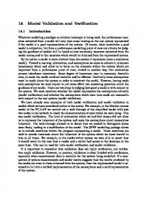
Test C2-Ex1: Channel infilling and migration: steady flow only 3.2.1 Purpose The CMS was applied to a laboratory flume study of channel infilling and migration due to a steady flow perpendicular to the channel axis. Model performance was evaluated by comparing measured and computed bed elevations of the channel cross-sections. Three channel cross-sections with slopes from 1:10 to 1:3 were simulated to test the limits of the depthaveraged model. Specific model features tested were: 1. Single-sized non-equilibrium total-load sediment transport, 2. Equilibrium inflow concentration boundary condition, and 3. Zero-gradient outflow boundary condition. 3.2.2 Experimental setup Three laboratory experiments of channel infilling and migration were carried out at the Delft Hydraulics Laboratory (DHL 1980) in a rectangular flume (length = 30 m, depth = 0.7 m, and width = 0.5 m) with a medium sand (d50 = 0.16 mm, d90 = 0.2 mm). In these tests, the mean flow velocity and water depth at the inlet were 0.51 m/sec and 0.39 m, respectively. The

14


initial channel cross-sections had side slopes of 1:10, 1:7 and 1:3. Sediment was supplied at a rate of 0.04 kg/m/sec at the inlet to avoid erosion. The upstream bed and suspended load transport rates were estimated at 0.01 and 0.03 kg/m/sec, respectively. 3.2.3 Model setup The laboratory study was simulated as a 1-D problem and the flume wall effects were ignored in the simulation for simplicity. The computational grid consisted of 3 rows and 220 columns (see Figure 5) with constant resolution of 0.1 m. The computational time step was 1 min. A flux boundary was specified for the upstream boundary with an equilibrium sediment concentration. Water level and zero concentration gradient boundary conditions were specified at the downstream boundary. Bed and suspended load scaling factors were adjusted to match the measured inflow transport rates and were estimated at 1.2 and 0.5 kg/m/sec, respectively. The Lund-CIRP transport formula (Camenen and Larson 2005, 2007, 2008) was used for all three cases. The transport grain size was set to median grain size (d50 = 0.16 mm), and no hiding and exposure were considered in the present simulations. The bed slope coefficient was set to 1.0. Sensitivity analysis shows that the model results were not sensitive to bed slope coefficients between 0.1 and 2.0. The bed porosity was estimated at 0.35. Representative settling velocity was 0.013 m/sec. A summary of selected model parameters is shown in Table 5. The total-load adaptation length was calibrated to 0.75 m using the measured bed elevations for Case 1, and then was applied in cases of side slopes 1:7 and 1:3 (Cases 2 and 3, respectively) to validate the model. 3.2.4 Results and discussion Cases 1, 2, and 3 correspond to the channels with side slopes equal to 1:10, 1:7 and 1:3, respectively. Since the depth-averaged CMS is expected to

Figure 5. Computational grid for the DHL (1980) experiment test case

15


16

Table 5. CMS-Flow parameter settings for DHL (1980) experiment test case. Parameter

Value

Flow time step

1 min

Simulation duration

15 hr


0.1 hr

Water density

1,000 kg/m3

Manning’s coefficient

0.025 sec/m1/3

Wall friction

Off

Transport grain size

0.16 mm

Bed slope coefficient

1.0

Sediment porosity

0.35

Sediment density

2,650 kg/m3

Suspended load scaling factor

1.2

Bed load scaling factor

0.5

Morphologic acceleration factor

1.0

Total load adaptation length

0.75 m

perform best for the cases without three-dimensional (3-D) flows caused by the steeper side slopes, Case 1 was chosen for calibration. Case 1 also has the most data of the three cases since bed elevations were measured at two elapsed times 3.2.4.1

Calibration

The only calibration parameter used was the total-load adaptation length which was estimated at 0.75 m. Computed and measured still-water depths for Case 1 are compared in Figure 6. The goodness-of-fit statistics for calculated water depth in Case 1 are given in Table 6. The Brier Skill Score (BSS) values indicate excellent model performance; however, it is recognized that these results were calibrated to best represent the measurements. 3.2.4.2

Validation

Computed and measured still-water depths for Cases 2 and 3 are compared in Figures 7 and 8. The corresponding goodness-of-fit statistics are given in Table 7. The model performance for Cases 2 and 3 was not as good as for Case 1, possibly due to flow separation on the upstream channel side caused by the steeper slopes of Case 3 and perhaps Case 2.


17

Figure 6. Measured and calculated bed elevations for Case 1 of DHL (1980). Table 6. Water depth goodness-of-fit statistics* for Case 1 of DHL (1980). Case 1

Time, hr

BSS

NRMSE, %

NMAE, %

R2

Bias, m

7.5

0.905

7.09

5.92

0.956

0.0010

15

0.932

7.75

5.77

0.955

-0.0031


Figure 7. Measured and calculated bed elevations for Case 2 of DHL (1980).


18

Figure 8. Measured and calculated bed elevations for Case 3 of DHL (1980). Table 7. Water depth goodness-of-fit statistics* for Cases 2 and 3 of DHL (1980). Case

Time, hr

BSS

NRMSE, %

NMAE, %

R2

Bias, m

2

15

0.888

10.21

7.55

0.880

-0.0005

3

15

0.795

20.19

15.36

0.623

-0.0098


When flow separation occurs, it is expected to cause a steepening of the upstream profile by hindering the downstream (downslope) movement of sediment at the upstream channel side. The presence of flow separation for Cases 2 and 3 is supported by the steep measured bathymetry. Since the CMS is a depth-averaged model, flow separation will cause significant errors in the computed morphology change. In general, flow separation is greatest at an incident current angle of 90 deg with respect to the channel axis and reduces as the angle decreases. Since most navigation channels at coastal inlets are approximately aligned with flow, flow separation may not be a major source of error in field applications. In applications with flow separation or other three-dimensional (3-D) flow patterns, a corresponding 3-D flow and sediment transport model may be necessary. 3.2.5 Conclusions and recommendations The CMS was applied to three laboratory cases of channel infilling and migration caused by steady flow. The model was calibrated using one case and validated using the other two cases. A good agreement was obtained


between computed and measured water depths, as indicated by the goodness-of-fit statistics in Tables 6 and 7. The best results were obtained for the mild (1:10) channel slope test case. Measured bed elevations for the channels with side slopes of 1:7 and 1:3 indicated flow separation which is not accounted for in the present depth-averaged model.

3.3

Test C2-Ex2: Channel infilling and migration: waves parallel to flow 3.3.1 Purpose The CMS was applied to a laboratory case to study channel infilling and migration with collinear steady flow and regular waves. Specific model features tested were: 1. Inline wave-current-sediment coupling, 2. The single-sized non-equilibrium total-load sediment transport model, and 3. Sediment boundary conditions. The model performance was tested using measured water depths and a sensitivity analysis was done for the transport formula, total-load adaptation length, and bed slope coefficient. 3.3.2 Experimental setup Van Rijn (1986) reported results from a laboratory experiment on the evolution of channel morphology in a wave-current flume caused by crosschannel flow and waves parallel to the flow. The flume was 17-m long, 0.3-m wide and 0.5-m deep. A pumping system was used to generate a steady current in the flume. The inflow depth-averaged velocity and water depth were 0.18 m/sec and 0.255 m, respectively. A circular weir was used to control the upstream water depth. Regular waves with a height of 0.08 m and period of 1.5 s were generated by a simple wave paddle. The bed material consisted of fine well sorted sand with d50 = 0.1 mm and d90 = 0.13 mm. Sand was supplied at a rate of 0.0167 kg/m/sec at the upstream end to maintain the bed elevation. A summary of the experiment hydrodynamic and wave conditions is presented in Table 8.

19


20

Table 8. Hydrodynamic and wave conditions for the van Rijn (1986) test case. Variable

Value

Upstream water depth

0.255 m

Upstream current velocity

0.18 m/sec

Wave height (regular)

0.08 m

Wave period (regular)

1.5 sec

Incident wave angle with respect to flow

0 deg

50th percentile (median) grain size, d50

0.1 mm

90th percentile grain size, d90

0.13 mm

3.3.3 Model setup For simplicity, the case was simulated as a 1-D problem by neglecting the flume wall effects. The computational grid had a constant resolution of 0.1 m, and was 3 cells wide (minimum for CMS) and 140 cells long (Figure 9). Water flux and equilibrium sediment concentration was specified at the upstream boundary, and a water level and zeroconcentration-gradient boundary was specified at the downstream end. Zero current velocity and water levels were specified as the initial condition (cold start). A summary of the relevant CMS-Flow and CMS-Wave settings is provided in Tables 9 and 10. The Lund-CIRP (Camenen and Larson2005, 2007, 2008), Soulsby-van Rijn (Soulsby 1997) (referred to as Soulsby for short), and van Rijn (van Rijn 1984ab; 2007b) transport formulas were used. Bed and suspended load transport scaling factors in Table 9 were adjusted to match the measured inflow sediment supply rate. Results are presented for a range of adaptation lengths and bed slope coefficients.

Figure 9. CMS computational grid for the van Rijn (1986) test case.


21

Table 9. CMS-Flow settings for the van Rijn (1986) test case. Parameter

Value

Solution scheme

Implicit

Time step

2 min

Simulation duration

10 hr


0.5 hr

Inflow discharge

0.0138 m3/sec

Outflow water level

-0.002 m

Manning coefficient

0.025 sec/m1/3

Wall friction

Off

Water density

1000 kg/m3


0.1 mm

Sediment transport formula

Lund-CIRP, Soulsby-van Rijn, and van Rijn

Bed and suspended load scaling factors

0.9 (Lund-CIRP) 2.7 (Soulsby-van Rijn), and 2.0 (van Rijn)


1.0

Sediment porosity, pm

0.3, 0.35, 0.4

Sediment density

2,650 kg/m3

Sediment fall velocity

0.007 m/sec

Bed slope coefficient, Ds

0, 1, 5

Total-load adaptation length, Lt

0.5, 1, 2, 5, and 10 m

Table 10. CMS-Wave settings for the van Rijn (1986) test case. Parameter

Value

Wave height (regular)

0.08 m

Wave period (regular)

1.5 sec

Incident wave angle with respect to flow

0.0 º

Bottom friction

Off

Steering interval

0.5 hr

3.3.4 Results and discussion The computed bed elevations after 10 hr for different transport formulas, adaptation lengths, bed slope coefficients, and porosities are shown in


Figures 10-13. The corresponding water depth goodness-of-fit statistics are provided in Tables 11-14. The results are consistent with those obtained by Sánchez and Wu (2011a) using a previous version of the CMS. The model reproduces the general trends of the morphology change including the upstream bank migration, channel infilling, and downstream bank erosion.

Figure 10. Measured and calculated water depths at 10 hr using the van Rijn transport formula and total-load adaptation lengths between 1 and 10 m.

Figure 11. Measured and calculated water depths at 10 hr using the Soulsby-van Rijn transport formula and total-load adaptation lengths between 1 and 10 m.

22


23

Figure 12. Measured and calculated water depths at 10 hr using the LundCIRP transport formula and total-load adaptation lengths between 0.5 and 5 m.

Figure 13. Measured and calculated water depths at 10 hr using the van Rijn transport formula and total-load adaptation length of 5.0 m and bed slope coefficient between 0 and 5. Table 11. Water depth goodness-of-fit statistics* using the van Rijn transport formula and varying total-load adaptation length. Total-load Adaptation Length, m

BSS

NRMSE %

NMAE %

R2

Bias m

1.0

0.453

23.50

20.78

0.700

-0.0008

2.0

0.686

13.50

11.15

0.876

0.0002

5.0

0.627

16.05

11.57

0.807

0.0015

10.0

0.471

22.73

17.46

0.766

0.0037



24

Table 12. Water depth goodness-of-fit statistics* using the Soulsby transport formula and varying total-load adaptation length. Total-load Adaptation Length, m

BSS

NRMSE %

NMAE %

R2

Bias m

1.0

-0.025

0.4407

0.3813

0.070

-0.0051

2.0

0.346

0.2812

0.2494

0.461

-0.0048

5.0

0.667

0.1433

0.1111

0.836

-0.0012

10.0

0.486

0.2210

0.1693

0.763

0.0026


Table 13. Water depth goodness-of-fit statistics using the Lund-CIRP transport formula and varying adaptation length. BSS

NRMSE %

NMAE %

R2

Bias m

0.5

0.458

0.2396

0.2042

0.909

0.0170

1.0

0.548

0.1998

0.1765

0.938

0.0147

2.0

0.514

0.2147

0.1671

0.866

0.0124

5.0

0.327

0.2973

0.2193

0.744

0.0098

Total-load Adaptation Length, m


Table 14. Water depth goodness-of-fit statistics* using the van Rijn transport formula as a function of varying bed slope coefficient. Bed slope Coefficient

BSS

NRMSE %

NMAE %

R2

Bias m

0.0

0.648

15.13

11.49

0.816

0.0012

1.0

0.669

14.25

10.59

0.834

0.0008

5.0

0.694

13.17

10.70

0.880

-0.0005


3.3.4.1

Transport formula and adaptation length

Among the three transport formulas, the van Rijn transport formula produced the best agreement as compared with measurements. The van Rijn and Soulsby transport formulas produced relatively similar results and were the best for a total-load adaptation length Lt = 5 m, while the LundCIRP formula provided the best results with Lt = 0.5 and 1 m, consistent with other similar experiments of channel infilling and migration. Of the three formulas tested, the Soulsby formula was the most sensitive to Lt and


produced a negative BSS (see Appendix A for definition) for Lt =1.0 m and less. The Lund-CIRP formula was the least sensitive to Lt. The differences in the best fit Lt for different transport formulas are due to differences in the transport capacities over the channel trough. The upstream concentration capacities were equal for all formulas since the bed and suspended load scaling factors were adjusted to match the measured sediment supply rate. These scaling factors were 2.0, 2.7, and 0.9 for the van Rijn, Soulsby, and Lund-CIRP transport formulas, respectively (see Table 9). Over the trough, the van Rijn, Soulsby, and Lund-CIRP formulas predicted concentration capacities equal to 0.051, 0.002, and 0.232 kg/m3, respectively. The van Rijn and Soulsby formulas estimated much smaller concentration capacities in the channel trough and produced greater channel infilling and migration than the Lund-CIRP formula. The van Rijn and Soulsby transport formulas also required larger transport scaling factors to match sediment supply rate (see Table 9). The adaptation length should be independent of the transport formula, yet the results show that errors from the transport formula may lead to different calibrated adaptation lengths. These results emphasize the importance of having an accurate transport formula. 3.3.4.2


The bed slope coefficient Ds is usually not an important calibration parameter for field applications. It has a default value of 1.0. Increasing the bed slope coefficient has the net effect of moving sediment downslope and smoothing the bathymetry. For this laboratory experiment case, the fraction of bed load upstream of the channel was approximately 8 to 17 percent. Although the best goodness-of-fit statistics were obtained from Ds = 5.0, it is clear from Figure 13 that this produced excessive smoothing as compared to Ds = 1.0. When the bed slope coefficient is turned off (Ds = 0.0), the calculated bed profile preserves the sharp corners from the initial profile but this is an unrealistic trend. 3.3.5 Conclusions and recommendations The CMS was applied to a laboratory experiment case of channel infilling and migration under steady flow and regular waves perpendicular to the channel axis (parallel to the flow). The non-equilibrium total-load sediment transport model was able to reproduce the overall morphologic behavior. A sensitivity analysis was conducted for three transport formulas, varying

25


total-load adaptation lengths and bed slope coefficients. The results show the importance of having an accurate sediment transport formula and how errors in the transport formula may lead to different calibration parameters. The bed slope coefficient is shown to be of secondary importance compared to the transport formula and adaptation length. For practical applications, running multiple simulations using different transport formulas and other model settings is recommended to assess the sensitivity of modeling results.

3.4

Test C2-Ex3: Channel infilling and migration: waves perpendicular to flow 3.4.1 Purpose The CMS was applied to a laboratory case of channel infilling and migration with steady flow and random waves. The case is similar to the previous one except that the waves were parallel to the channel axis (perpendicular to flow). Specific model features tested in this case were: 1. Inline wave-current-sediment coupling, 2. Single-sized non-equilibrium total-load transport model, and 3. Sediment boundary conditions. The model performance was evaluated using measured water depths and a sensitivity analysis was performed for the total-load adaptation length. 3.4.2 Experiment Van Rijn and Havinga (1995) conducted a laboratory experiment on the channel morphology change under steady cross-channel flow with waves perpendicular to the flow. The flume was approximately 4 m wide and had 1:10 side slopes. The depth-averaged current velocity and water depth at the inlet were 0.245 m/sec and 0.42 m, respectively. Random waves (JONSWAP form) were generated at a 90 deg angle to the flow and had a significant wave height of 0.105 m and peak wave period of 2.2 sec. The suspended sediment transport rate was measured to be at 0.022 kg/m/sec. Table 15 summarizes the experimental conditions.

26


27

Table 15. General conditions for van Rijn and Havinga (1995) experiment. Parameter

Value

Upstream current velocity

0.245 m/sec

Upstream water depth

0.42 m

Significant wave height

0.105 m

Peak wave period

2.2 sec

Wave direction

90º

Upstream suspended transport rate

0.022 kg/m/sec

Median grain size

0.1 mm

3.4.3 Model setup For simplicity, the case was simulated as a 1-D problem by ignoring the flume wall effects. The same computational grid used for CMS-Flow and CMS-Wave is shown in Figure 14 with the colors representing the initial bathymetry. The grid had 390 active computational cells and a constant resolution of 0.1 m. A water flux boundary condition was used at the upstream boundary (left side) and a water level boundary at the downstream boundary (right side). The initial condition was specified as zero for water level and current velocity over the whole grid. Equilibrium sediment concentration was specified at the inflow boundary and a zerogradient boundary condition at the outflow boundary.

Figure 14. CMS computational grid for the van Rijn and Havinga (1986) test case.

Table 16 shows CMS setup parameters. Default CMS values were used wherever possible. The Manning’s coefficient was estimated as 0.02 sec/m1/3 by fitting a lognormal distribution to the measured current velocity profile. The suspended-load scaling factor was adjusted based on the measured inflow transport rate and set to 0.67, which is within the generally accepted range of 0.5 to 2.0. Since no measurements for bed load were available, the bed-load transport capacity was not modified. The


28

transport grain size was set to median grain size so that no hiding and exposure was considered in the simulation. Model result sensitivity to the adaptation length Lt was tested for the values of 0.5, 0.7, 1, and 2 m, as shown in Table 16. 3.4.4 Results and discussion Figure 15 shows a comparison of the measured and computed bed elevations after 23.5 hr for each adaptation length evaluated. The results are consistent with those obtained by Sánchez and Wu (2011a) with a previous version of the CMS. The model reproduces the overall measured trend of the channel migration and infilling. However, the computed bathymetry is much smoother than the measured bathymetry. This is due to the fact that the model does not simulate the small-scale bed forms. Table 16. CMS-Flow input settings for the Van Rijn and Havinga (1995) test case. Setting

Value

Solution scheme

Implicit

Simulation duration

24 hr


30 min

Time step

1 min


0.02 sec/m1/3

Steering interval

3 hr


0.1 mm

Transport formula

Lund-CIRP


1.0


0.67


1.0


0.6 mm/sec

Bed porosity

0.4


1.0

Total-load adaptation length, Lt

0.5, 0.7, 1, 2 m


29

Figure 15. Measured and calculated bathymetry at 23.5 hr with varying total-load adaptation lengths between 0.5 and 2.0 m.

Based on the goodness-of-fit statistics shown in Table 17, the model performance is relatively good. For this case, adaptation lengths of 0.5, 0.7, and 1 m gave similar results. The results show that the model results can be sensitive to the adaptation length. However, once this parameter is calibrated, relatively accurate results may be obtained. This parameter is difficult to estimate because it depends on the vertical structure of currents, sediment concentration, and turbulence, which are difficult to assess with a depth-averaged model. Table 17. Water depth goodness-of-fit statistics* for the Van Rijn and Havinga (1995) experiment. Total-load Adaptation Length, m

BSS

NRMSE, %

NMAE, % R2

Bias, m

0.5

0.978

15.60

12.55

0.897

0.0071

0.7

0.983

13.85

12.02

0.876

0.0063

1.0

0.976

16.37

12.91

0.754

0.0054

2.0

0.917

30.49

22.91

0.252

0.0039


3.4.5 Conclusions and recommendations The CMS model performance in simulating channel infilling and migration was assessed with a laboratory flume experiment case under random waves and steady flow. The waves in this case were perpendicular to the direction


of the flow. Coupled waves, currents, and non-equilibrium sediment transport were simulated with the inline CMS (single code), and computed water depths were compared to measurements. The goodness-of-fit statistics for the water depths indicates good model performance for totalload adaptation lengths from 0.5 to 1.0 m. For practical applications it is important to calibrate the adaptation length using measured morphology changes. Future research will be directed towards better understanding and predicting the adaptation length for a wide variety of conditions.

3.5

Test C2-Ex4: Large-scale sediment transport facility 3.5.1 Purpose Data from the Large-Scale Sediment Transport Facility provide detailed measurements of wave height, water level, longshore current speed, and sediment transport (bed- and suspended-load) within a controlled laboratory environment. Application of the CMS to this test case demonstrated the model capability of calculating the cross-shore distribution of wave height, longshore current, and sediment transport from the wave breaker zone inshore. 3.5.2 Experimental setup The Large-Scale Sediment Transport Facility (LSTF) at ERDC (see Figure 16) is capable of simulating oblique (6.5 deg incident angle) regular and random waves, and a uniform longshore current. The longshore current is recirculated from the downdrift end to the updrift end of the LSTF by adjusting a series of 20 pumps in the cross-shore direction, therefore simulating an infinite beach. The test case discussed here represented a natural beach with a uniform longshore current. The experiment was 160 min long and measured the cross-shore distribution of significant wave height, water level, current speed, and suspended-sediment transport. All comparisons here are for Case 1, in which a longshore current was induced by oblique random waves and the pumps were adjusted to match the measured longshore current. Table 18 summarizes the setup for LSTF Case 1.

30


31

Figure 16. LSTF configuration (Gravens and Wang 2007). Table 18. Wave and hydrodynamic conditions for LSTF Test Case 1. Variable

Value

Offshore significant wave height, Hs

0.228 m

Peak period, Tp

1.465 sec

Incident wave angle, Θo

6.5o

Water level, η0

-0.001 m

3.5.3 Model setup The computational domain was generated based on the interpolation of measured beach profiles from profile Y14 to Y34 (see Figure 16). A constant grid resolution of 0.2 and 0.4 m was used in the cross-shore and longshore directions, respectively. A TMA spectrum was assumed at the offshore boundary with the parameter values γ = 3.3, and n = 100. The offshore water level during the experiment was not equal to the Still Water Level (SWL) because of the wave setup. The offshore water level was approximated for each experiment based on the most offshore water level gauge. Tables 19 and 20 summarize the CMS-Flow and CMS-Wave settings, respectively.


32

Table 19. CMS-Flow settings for the LSTF test cases. Setting

Value

Solution scheme

Implicit

Time step

1 min

Wetting and drying depth

0.001 m

Simulation duration

3.0 hr

Ramp duration

2.5 hr

Manning coefficient

0.016 sec/m1/3


0.15 mm

Transport formula

Lund-CIRP, van Rijn, and Soulsby-van RIjn

Sediment porosity

0.4


0.0 (no bed change)

Table 20. CMS-Wave settings for the LSTF test cases. Setting

Value

Wave breaking

Battjes and Janssen (1978)

Bottom friction

Off

Steering interval

0.25 hr

Roller

On

Roller dissipation coefficient

0.1

Roller efficiency factor

1.0

3.5.4 Results and discussion Calculated wave heights, depth-averaged current velocities, and water levels are compared with the LSTF center line profile measurements in Figures 17 through 19. Table 21 summarizes the goodness-of-fit statistics for hydrodynamics in Case 1. Wave heights and water levels have normalized errors of 3 to 4 percent and 10 to 12 percent, respectively. Similar results were obtained by Nam et al. (2009). Longshore current calculations have larger errors ranging from 18 to 24 percent. The calculated peak longshore current is slightly offshore from the measured peak. Reducing the roller dissipation coefficient may improve these estimates by moving the peak longshore current closer to the shoreline. Another reason is that the location of the second breaker zone, located at approximately 6 to 7 m from the shoreline, is predicted slightly further offshore, causing the a longshore current peak which is also further offshore.


Figure 17. Measured and computed significant wave heights for LSTF Case 1.

Figure 18. Measured and computed longshore currents for LSTF Case 1.

Figure 19. Measured and computed mean water levels for LSTF Case 1.

33


34

Table 21. Goodness-of-fit statistics* for waves, water levels and longshore currents in LSTF Case 1. Hs

Water Level

Longshore Current

NRMSE, %

3.63

12.18

24.09

NMAE, %

3.15

9.86

18.09

R2

0.982

0.934

0.665

Bias, m, m/sec

-0.005

0.0001

0.017


Figures 20 through 22 show comparisons between calculated and measured suspended sediment transport in the longshore direction using three sediment transport formulas: Lund-CIRP (Figure 20), Soulsby-van Rijn (Figure 21), and van Rijn (Figure 22). The measurements show three peaks in the sediment transport magnitudes, one near the offshore bar, another in the middle of the profile where there is a very slight inshore bar, and the greatest value at the swash zone. All three formulations predict well the locations of the two offshore peaks but underestimate the sediment transport near the shoreline. This is due to the fact that the swash zone is not included in the present CMS. Nam et al. (2009) found similar results without the swash zone transport and also obtained significantly improved results by including the swash zone sediment transport. The swash zone sediment transport not only increases the transport in the swash zone but also in the surf zone by acting as a concentration boundary condition to the transport equation in the surf zone.

Figure 20. Measured and computed longshore sediment transport rates in LSTF Case 1 using the Lund-CIRP formula.


Figure 21. Measured and computed longshore sediment transport rates in LSTF Case 1 using the Soulsby-van Rijn formula.

Figure 22. Measured and computed longshore sediment transport rates in LSTF Case 1 using the van Rijn formula.

In the present version of CMS, the wave height and current velocity will always tend to go to zero towards the shoreline, leading to an underprediction of the transport. The Lund-CIRP and Soulsby-van Rijn formulas predict well the magnitude of the transport while the van Rijn formula underpredicts the transport by a factor of about two. It is interesting to note that, even though the location of the peak longshore current is not well predicted, the location of the peak longshore sediment transport is well predicted. Table 22 summarizes the goodness-of-fit statistics for the sediment transport calculations. All formulas have a negative bias, meaning that they all underpredict the magnitude of the mean sediment transport. Errors range from 22 to 26 percent, 26 to 33 percent, and 35 to 40 percent for the Lund-CIRP, Soulsby-van Rijn, and van Rijn formulations, respectively.

35


36

Table 22. Sediment transport goodness-of-fit statistics* for LSTF Case 1. Statistic

Lund-CIRP

NRMSE, %

25.88

32.02

33.77

NMAE, %

21.99

26.01

29.81

R2

0.164

Bias, m3/m/year

2.79

Soulsby-van Rijn

0.097 -23.38

van Rijn

0.567 -66.80


3.5.5 Conclusions and recommendations The CMS was applied to LSTF Case 1 to compare with measured wave height, longshore current speed, water level, and sediment transport rate. Hydrodynamic comparisons were good, with errors of 3 to 4 percent and 9 to 12 percent for wave height and water level, respectively. Calculated longshore current speed agreed with measurements near the breaker line and into the surf zone, but the calculated peak current speed was offshore from the measurements, resulting in errors ranging from 18 to 24 percent. Calculations of sediment transport were conducted using three different formulas available in CMS. All formulas had a negative bias, meaning that they all underpredicted the magnitude of the mean sediment transport. Errors ranged from 22 to 26 percent, 26 to 32 percent, and 30 to 34 percent for the Lund-CIRP, Soulsby-van Rijn, and van Rijn formulas, respectively. Sediment transport calculations using the Lund-CIRP and Soulsby-van Rijn were in better agreement from the breaker zone to midway through the surf zone. All formulas underpredicted sediment transport near the shoreline due to the lack of swash zone processes, which are presently being implemented in CMS. When calibrating the net longshore sediment transport from CMS to estimates from sediment budgets, it is important to take into account that the CMS will tend to underpredict the longshore sediment transport due to the missing swash zone processes. As the LSTF experiments show, the longshore sediment transport in the swash zone can be significant and even larger than that in the surf zone. These tests demonstrate that CMS can be applied to calculate nearshore hydrodynamics and sediment transport within the calculated error bounds.


3.6

37

Test C2-Ex5: Clear water jet erosion over a hard bottom 3.6.1 Purpose The CMS was applied to a laboratory case of a clear water jet in a rectangular flume with a sandy bed layer over a hard bottom. The experiment is good for testing the sediment transport model under strong erosion conditions in the presence of a hard bottom. 3.6.2 Experimental setup Thuc (1991) carried out a movable bed laboratory experiment in a rectangular flume 5-m long and 4-m wide, with a narrow 0.2-m-wide inlet and a 3-m-wide outlet. The initial water depth was 0.15 m, with a 0.16-m layer of sand (d50 = 0.6 mm) over a concrete bottom. The estimated sand settling velocity is 0.013 m/sec. Hydrodynamic and sediment parameters for the experiment are summarized in Table 23. Table 23. Hydrodynamic and sediment conditions for the Thuc (1991) experiment case. Parameter

Value

Inflow depth-averaged current velocity

0.6 m/sec

Initial water depth

0.15 m

Bed median grain size

0.6 mm

Representative sediment fall velocity

0.013 m/sec

Bed layer thickness

0.16 m

3.6.3 Model setup The transport equation which best fit the measurements was the Soulsbyvan Rijn (Soulsby 1997). No measurements of bed- or suspended-load were available. It was found that the best morphologic results were obtained with bed- and suspended-load scaling factors of 2.0, which are within the typical accepted range of 0.5 to 2.0. The total-load adaptation length was calculated based on a weighted averaged of the bed and suspended-load adaptation lengths. The suspended-load adaptation length was calculated using the Armanini and di Silvio (1986) formula. The bedload adaptation length was set to the local water depth. The bed slope coefficient was set to 0.5. Sensitivity analysis showed that the results were not sensitive to the bed slope coefficient. The parameters used are listed in Table 24. The model setup and results shown here are the same as those presented in Wu et al. (2010).


38

Table 24. Hydrodynamic and sediment parameters for the Thuc (1991) experiment case. Parameter

Value

Solution scheme

Implicit

Time step

30 s

Simulation duration

4.25 hr


0.01 hr


0.03 sec/m1/3


0.6 mm


0.013 m/sec

Sediment density

2,650 kg/m3

Sediment porosity

0.4

Bed and suspended load scaling factors

2.0


1.0

Sediment inflow loading factor

0.0 (clear water)

Total load adaptation coefficient method

Weighted average of bed and suspended load adaptation lengths

Suspended load adaptation coefficient method

Armanini and di Silvio (1986)

Bed load adaptation length

Equal to local water depth

Avalanching

On

The computational grid (see Figure 23) had a constant resolution in the x-direction of 0.1 m and a variable resolution in the y-direction between 0.0333 and 0.1333 m. The computational mesh consisted of 62 rows and 69 columns. The computational time step was 30 sec. A water flux boundary was applied at the upstream end and a water level boundary was applied to the downstream end. The initial water level and current velocities were set to zero for the whole domain (cold start). 3.6.4 Results and discussion Figure 24 shows the calculated flow pattern in the domain and bed change contours around the inflow region at the center part of the basin after an elapsed time of 4 hr. Similar results were obtained by Min Duc et al. (2004) and Wu (2004). Erosion occurred due to the inflow of clear water, and the eroded sediment moved downstream and deposited forming a dune feature which migrated slowly downstream. The results show good symmetry about the centerline. Figure 25 compares the measured and calculated bed changes along the longitudinal centerline at 1 and 4 hr. The calculated erosion and deposition depths are in good agreement with the measured data, in particular at time 4 hr. The goodness-of-fit statistics for the computed water depth is shown in Table 25.


Figure 23. Computational grid for the Thuc (1991) experiment case.

Figure 24. Computed bed elevations and current velocities at 4 hr for the Thuc (1991) test case.

Figure 25. Comparison of calculated and measured bed elevations at 1 and 4 hr for the Thuc (1991) test case.

39


40

3.6.5 Conclusions and recommendations The laboratory experiment of Thuc (1991) was simulated with the CMS. The water depth BSSs calculated at 1 and 4 hr were good and demonstrated excellent model performance, respectively (see Appendix A). The water depth NMAEs were approximately 19 and 6 percent at 1 and 4 hr, respectively. The sediment inflow loading factor was used to apply a clearwater boundary condition. Two important model features were tested, hardbottom and avalanching, both of which performed satisfactorily. Table 25. Water depth goodness-of-fit statistics* for the Thuc (1991) test case. Time, hr

BSS

NRMSE, %

NMAE, %

R2

Bias, m

1.0

0.411

26.95

19.32

0.413

-0.023

4.0

0.941

8.52

5.60

0.956

-0.0012


3.7

Test C2-Ex6: Bed aggradation and sediment sorting 3.7.1 Purpose The CMS was applied to three laboratory cases of channel deposition with multiple-sized sediments. The laboratory experiments are useful for testing the non-uniform sediment transport under transcritical flow conditions. The specific model features tested were the multiple-sized sediment transport, bed change, and bed material sorting algorithms. 3.7.2 Experiment setup Laboratory experiments of bed aggradation and sediment sorting were carried out at the St. Anthony Falls Laboratory (SAFL) by Paola et al. (1992) and Seal et al. (1995). The flume was 45-m long and 0.305-m wide, as shown in Figure 26. A tailgate was used to keep the downstream end at a constant water level. The inflow water flux was 0.049 m3/sec. The initial bed slope was 0.002. A slightly bimodal mixture of sediments ranging in size from 0.125 to 64 mm was fed into the flume. A summary of the experimental conditions for the three SAFL cases used here is provided in Table 26.


41

3.7.3 Model setup The CMS-Flow computational grid for the rectangular flume was 3-cellswide and 100-cells-long, which were of size 0.5 m by 0.1 m in x- and ydirections, respectively (see Figure 27). A constant flux boundary condition was applied at the upstream end and a constant water level boundary condition was applied at the downstream end of the flume. A 1-hr ramp period was necessary to stabilize the hydrodynamics. During this ramp period, the sediment transport equation was solved but the bed elevation was not updated. In addition, a relatively small time step of 1 sec was necessary to stabilize the flow due to the transcritical flow. A summary of the selected hydrodynamic and sediment transport parameters is presented in Table 27. The laboratory study was simulated as a 1-D problem and the flume wall effects were ignored in the simulation for simplicity and, therefore, wall friction is lumped into the bottom friction. A Manning’s roughness coefficient of 0.028 sec/m1/3 was estimated based on the measured flow depths and bed slopes.

Figure 26.Sketch of the SAFL channel aggradation experiment. Table 26. Hydrodynamic and sediment conditions for the three simulated SAFL cases. Variable

Case 1

Case 2

Case 3

Experiment duration, hr

16.83

32.4

64

Inflow discharge, l/sec

49

49

49

Initial bed slope

0.002

0.002

0.002

Downstream water level, m (from bed)

0.4

0.45

0.5

11.3

5.65

2.83

Initial d50 (50th percentile), mm

5.9

5.9

5.9

Initial d90 (90th percentile), mm

33.1

33.1

33.1

Sediment feed rate, kg/min

Geometric standard deviation, mm

5.57

5.57

5.57


42

Figure 27.CMS-Flow computational grid for the SAFL test cases.

A fractional sediment transport rate was applied at the inflow boundary using the sediment feeding rate and the grain size distribution shown in Figure 28. The grain size distribution consisted of nine sediment size classes from 0.177 to 45.25 mm. A zero-gradient concentration boundary condition was applied at the downstream end. The initial bed material Table 27. CMS-Flow settings for the SAFL experiment test case. Parameter

Value

Time step

1s

Simulation duration

Case 1: 18 hr Case 2: 34 hr Case 3: 65 hr


1 hr


0.028 sec/m1/3

Wall friction

Off

Water density

1,000 kg/m3

Transport formula

van Rijn


0.0

Number of sediment size classes

9

Porosity

0.3

Sediment density

2,650 kg/m3


1.0


1.0


1.0

Inflow loading factor

0.9

Morphologic update during ramp period

Off

Total-load adaptation length

0.9 m

Hiding and exposure coefficient

0.2

Minimum bed layer thickness

0.01 m

Maximum bed layer thickness

0.1 m

Number of bed layers

19


43

20

Fraction, %

15 10 5 0 -1 10

0

1

2

10 10 10 Grain size, mm Figure 28.Grain size distribution of the sediment supplied at the upstream end of the flume for the SAFL test cases.

composition was set to the sediment supply distribution. To account for the sediment that rolled backward at the feeding location, an inflow loading factor of 0.9 was applied, meaning 10 percent of the sediment feeding was assumed to role backward. The van Rijn (1984a, b; 2007a, b) transport formula was applied. The transport formula was modified to account for hiding and exposure by multiplying the critical velocity by a correction factor calculated based on Wu et al. (2000). 3.7.4 Results and discussion Case 2 was chosen for calibration because its hydrodynamic conditions are in between Cases 1 and 3 and is, therefore, the most representative of the group (see Table 26). Cases 1 and 3 were run using the same settings and parameters as Case 2 and serve as model validation. 3.7.4.1

Calibration

Calibration was carried out by first selecting a transport capacity formula and adjusting the bed- and suspended-load transport scaling factors. For simplicity, the same scaling factor was applied to both the bed and suspended load. The van Rijn transport capacity formula with default transport scaling factors of 1.0 was found to provide the best results. Secondly, the total-load adaptation length was adjusted based on the morphology change to 0.9 m, which is very close to other laboratory experiments presented in this report. Lastly, the exponent coefficient used for correcting the critical velocity for hiding and exposure was adjusted to match the measured gain size distribution and was found to be approximately 0.2.


Figure 29 shows a comparison of the calculated and measured bed profiles and water levels for Case 2. The rectangles represent bed layers with colors indicating the median grain size (d50). The corresponding goodness-of-fit statistics are given in Table 28.Calculated bed elevations have normalized errors less than 5 percent and BSSs larger than 0.897. CMS-Flow was able to reproduce the vertical bed aggradation, downstream migration of the depositional fan, the bed slope, and mildly concave bed profile. The final bed material composition is characterized by coarser (finer) sediments upstream (downstream) and upward (downward) due to selective sediment transport and bed sorting. The water level profile is characterized by a hydraulic jump near the tip of the depositional fan. Calculated water levels were accurate with a NMAE of 3 percent. Interestingly, the bed profile was found to not be significantly sensitive to the hiding and exposure coefficient and was most sensitive to the bed- and suspended-load transport scaling factors, and to lesser extent the totalload adaptation length. The hiding and exposure coefficient did however have a large influence on the bed composition (grain size distribution).

Figure 29. Measured and computed bed elevations and water levels at different elapsed times for the SAFL experiment Case 2. Colored rectangles indicate bed layers with colors corresponding to the median grain size at 32.4 hr.

44


45

Table 28. Goodness-of-fit statistics* for the SAFL experiment Case 2. Bed level, m 16

Water Level, m

d50, mm

d90, mm

32.4

32.4

32.4

Time, hr

4

32.4

BSS

0.911

0.897

0.920

0.940

NRMSE, %

2.28

4.31

4.88

2.58

57.79

35.28

NMAE, %

1.54

2.86

3.02

2.13

53.48

34.04

R2

0.994

0.984

0.977

0.995

0.549

0.217

Bias

-0.0020

-0.0011

-0.0088

-0.0061

1.1132

4.6798

0.782

0.067


Figure 30 compares the calculated and measured bed surface d50 and d90 at 32.4 hr. There is a noticeable increase in both d50 and d90 from the initial bed size. Measured d50 grain size shows a downstream fining from approximately 16 to 12 mm, while d90 shows a larger downstream decrease from approximately 55 to 30 mm. The calculated d50 grain size has a NMAE, BSS, and R2 of approximately 53 percent, 0.78, and 0.55, respectively. 60

Grain size, mm

50

Measured d50 Measured d90

40

Calculated d50

30

Calculated d90 Initial d50

20

Initial d90

10 0

0

5

10

15 20 Distance, m

25

30

Figure 30. Measured and computed d50 and d90 grain sizes for the SAFL Case 2.

The d50 bias is approximately one third the measure data range. The calculated d90 grain size has a lower NMAE of 34 percent compared to d50, but has a lower BSS and R2 but a smaller NMAE. The d90 bias of 4.7 mm is approximately one fifth the measured data range. Both the calculated d50 and d90 show a slight increase up to about 14 to 16 m downstream followed by a relatively steep decrease. The reason for this is not understood and further investigation is needed. However, it is interesting to note that the measured d90 grain size also shows a slight increase from 10 to 17 m. The bed composition however, was sensitive to the hiding and exposure correction factor.


One possible reason why the bed composition was not sensitive to the bed and suspended transport scaling factors is because the same values were applied to all grain sizes. It is expected that improved grain size distributions can be obtained with grain-size-dependant transport scaling factors. However, since no fractional sediment transport rates were available, it was not possible to estimate these factors. For most practical applications, detailed fractional sediment transport rates are not available and, therefore, using constant transport scaling factors is sufficient. 3.7.4.2

Validation

The calculated and measured bed profiles and water levels for the validation Case 1 are presented in Figure 31. Case 1 corresponds to the experiment case with the largest sediment feeding rate and lowest tail gate water level. The corresponding goodness-of-fit statistics are given in Table 29. Similar to Case 2, the calculated bed elevations have normalized errors less than 4 percent and BSSs between 0.87 and 0.924. CMS-Flow was able to reproduce the bed slope and mildly concave bed profile.

Figure 31. Measured and computed bed elevations and water levels at different elapsed times for the SAFL experiment Case 1. Colored rectangles indicate bed layers with colors corresponding to the median grain size at 16.83 hr.

46


47

Table 29. Goodness-of-fit statistics* for the SAFL Case 1. Bed level, m

Water Level, m

d50, mm

d90, mm

Time, hr

2

8

16.83

16.83

16.83

16.83

BSS

0.870

0.914

0.924

0.928

-3.78

-0.838

NRMSE, %

3.54

3.74

3.90

3.07

156.19

53.93

NMAE, %

2.90

2.62

2.44

2.36

152.22

47.50

R2

0.990

0.989

0.982

0.995

0.129

0.888

Bias

-0.0058

-0.0031

0.0062

0.0077

5.92

10.14


The vertical bed aggradation and downstream migration of the depositional fan were slightly over predicted. Similarly to Case 2, the bed material composition is characterized by coarser (finer) sediments upstream (downstream) and upward (downward) due to selective sediment transport and bed material sorting. The calculated upstream water levels and downstream location of the hydraulic jump were over predicted slightly due to the over predicted bed elevation and deposition fan migration, respectively. However, in general, the water level goodness-of-fit statistics indicate good model performance with a BSS of 0.928, a NMAE of 2.36 percent, and R2 of 0.995. The calculated and measured bed surface d50 and d90 for Cases 1 are shown in Figure 32.The corresponding goodness-of-fit statistics are given in Table 29. Surprisingly, the measured d50 is approximately the same as the initial d50. The calculated d50 is over predicted, closer to that of Case 2, at around 11 mm, and has a slight increase before decreasing at a distance of approximately 25 m. The calculated d90 is within the measured range upstream (x

Verification and Validation of the Coastal Modeling System; Report 4

Verification and Validation of the Coastal Modeling System; Report 4

Suggest Documents

Verification and Validation of the Coastal Modeling System; Report 3 ...

Verification and Validation of the Coastal Modeling System; Report 3

Closed-loop System Modeling, Validation, and Verification - Uni Halle

Modeling and Simulation Verification and Validation Challenges

Verification and Validation Report: Frequency Selective Surface ...

Vehicle Speed Meters Validation and Verification System

Verification, validation, and certification of modeling and ... - IEEE Xplore

2004: Quality Assessment, Verification, and Validation of Modeling

2004: Quality Assessment, Verification, and Validation of Modeling ...

Validation and Verification - CiteSeerX

Method validation and verification

Method validation and verification

Data Verification and Validation Process in the Management System

Expert system verification and validation - University of Southern ...

Verification and validation of a FDD system for ... - eLib - DLR

'verification and validation' in modeling fire by ... - Semantic Scholar

'verification and validation' in modeling fire by ... - Semantic Scholar

Expert system verification and validation: a survey and ... - CiteSeerX

A coordinated coastal ocean observing and modeling system for the ...

A Coastal Ocean Observing System and Modeling Program for the ...

SIMULATION MODEL VERIFICATION AND VALIDATION ...

Software Testing: Verification and Validation

14 Model Validation and Verification

14 Model Validation and Verification