Verification of Concurrent Systems with Parametric Delays ... - UOC

Verification of Concurrent Systems with Parametric Delays Using Octahedra Robert Claris´o and Jordi Cortadella∗ Universitat Polit`ecnica de Catalunya Barcelona, Spain Abstract A technique for the verification of concurrent parametric timed systems is presented. In the systems under study, each action has a bounded delay where the bounds are either constants or parameters. Given a safety property, the analysis computes automatically a set of constraints on the parameters sufficient to guarantee the property. The main contribution is an innovative representation of the parametric timed state space based on bit-vectors. Experimental results from the domain of timed circuits show that this representation improves both CPU time and memory usage with respect to another parametric approach, convex polyhedra.

TRAIN

far

] exit

[0,+

app [0,+

]

near

inside enter [dE ,DE ] GATE raise [dC ,DC ]

closed

up [dR ,DR ]

goingup

lower

raise far

[dC ,DC ]

near

open

[dC ,DC ]

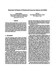
1. Introduction The behavior of many concurrent systems depends on their temporal characteristics. Many real-time formalisms describe these characteristics using bounded delays (e.g. timed transition systems [16]) or clocks whose value can be read or reset (e.g. timed automata [2]). In these formalisms, the delays and clock thresholds are usually defined as known constants. A more general class of models is that of parametric real-time systems [3], where these values become parameters of the problem. In addition to simply checking whether a temporal property is satisfied by a parametric system, it is also possible to compute which values of the parameters satisfy the property. For example, let us consider the timed Petri Net in Figure 1 depicting the railroad crossing problem. The subnet on the top describes the behavior of a train as it approaches a crossing. The subnet on the bottom depicts the behavior of the gate at the crossing. Each event has a delay bounded by an interval [d, D], which captures the amount of time elapsed since the event becomes enabled until it occurs. Some bounds of the intervals are parameters of the problem: the time required to lower and raise the gate ([dL , DL ] and [dR , DR ] respectively), the time required by the controller of the gate to issue a command ([dC , DC ]) and the time between the sensor detects the proximity of the train until the train enters the crossing ([dE , DE ]). The following safety property should be satisfied: “whenever the train is inside the crossing, the gate should be closed”. The analysis described in this paper is able to discover the safety requirement (dE > DL + DR + DC ) automatically. ∗ Research funded by CICYT TIN 2004-07925 and the FPU grant AP2002-3862 from the Spanish Ministry of Education, Culture and Sports.

down [dL ,DL ]

goingdown

lower [dC ,DC ]

Figure 1. The railroad crossing problem

Techniques used in real-time systems such as Difference Bound Matrices (DBMs) [14] cannot be used to study parametric systems. These methods can only handle constraints that involve at most two variables, while in parametric systems several parameters may appear in the same constraint. Furthermore, many interesting problems for parametric timed systems are undecidable. As such, it is only possible to address them using approximate techniques (e.g. [1]) or semi-decision procedures (e.g. [5]). This paper focuses on the verification of a specific class of timed systems: timed circuits [18]. They rely on timing constraints to ensure a correct operation. Timing constraints limit the degree of concurrency in the circuit: some behaviors valid in the untimed domain become forbidden in the timed domain. The results presented in this paper extend the approach presented in [10]. This method, based on abstract interpretation [11], discovers a very general class of timing constraints that can be used later to: • Efficiently check if an implementation of a circuit with specific delays satisfies the timing constraints. • Choose which delays should be used in the implementation in order to improve performance, while ensuring a correct functionality. This method does not impose a priori any restriction on the delays of the elements of the circuit. Instead, delays are modeled as symbols. The output timing constraints are linear inequalities describing a set of sufficient constraints on these symbols that guarantee a correct behavior. Notice that

D

C

E

s

y

∆ x+

x−

le out

le+

y+

>

δ(B)

>

δ(x−)

re re+

x le−

y−

δ(x−) δ(B) + δ(not) + δ(F )

re−

A B not

Right environment

a

Left environment F

Pulse signal to data latch

δ(y+)

>

δ(E)

δ(y−) + δ(A)

>

δ(∆) + δ(D) + δ(C)

δ(∆)

>

δ(not) + δ(C)

δ(y+)

>

δ(∆)

δ(x+)

>

δ(not) + δ(C)

δ(x+)

>

δ(∆) + δ(D) + δ(C)

δ(x+)

>

δ(y+) + δ(A) + δ(y−)

δ(D) + δ(∆)

>

δ(A)

δ(y−)

>

δ(not) + δ(B) + δ(C)

Figure 2. GasP FIFO controller [22]. Each shaded area has been modeled with a different symbolic delay. On the right, the timing constraints that ensure a correct operation of the circuit.

this kind of timing constraints is less restrictive than metric timing constraints1 [6, 7] and easier to validate than relative timing constraints2 [19, 21]. This additional freedom can be used to select more aggressive delays for larger performance gains.

1.1. Motivating example: GasP FIFO controller The approach presented in this paper is suitable for the verification of small controllers, typically designed by hand or by sophisticated synthesis tools, whose behavior depends on the timing characteristics of the components, such as asynchronous controllers (e.g. [20, 22]). For example, Figure 2 shows a GasP FIFO controller [22]. The environment of this controller is modeled with Signal Transition Graphs (STG) [8]. Gates, transistors and environment events have a delay specified as a symbol (δ). The correctness of the circuit has been verified with respect to three criteria: absence of short-circuits; absence of hazards; and conformance, i.e. all output events produced by the circuit are expected by the environment. These criteria can be satisfied with the timing constraints that appear in Fig.2. For example, the constraint (δ(x−) > δ(B)) models the fact that changes in the input signal x must be slow enough to let the transistor B discharge the signal le. On the other side, the constraint (δ(B) + δ(not) + δ(F ) > δ(x−)) establishes that the event x− must be faster than the path defined by the transistor B, the inverter and the pair of transistors in F . Otherwise, there is a short-circuit as transistors B and C may be both on.

1.2. The contribution The main contribution of this paper is the innovative representation for the linear timing constraints presented 1 Setting the lower and upper bound delays of each element, or introducing constant delay paddings to ensure correctness. 2 Restrictions on the relative order of concurrent events.

in Section 3. Instead of using linear constraints, only unit constraints, i.e. linear constraints with coefficients {−1, 0, +1}, are considered. This restriction is useful because most timing constraints are implicitly comparing the delay of two paths in the circuit: (δ1 + · · · + δi ) − (δi+1 + · · · + δn ) ≥ k
 
  delay(path1) delay(path2) The encoding of unit constraints is based on bit-vectors and it improves memory and time usage with respect to previous representations based on convex polyhedra [10] and decision diagrams [9], although it may generate more restrictive timing constraints. Using this new method, larger circuits which were not analyzable previously can be successfully studied. Furthermore, the analysis of other types of parametric timed systems, such as parametric timed automata, can also benefit from this enconding.

2. Timing analysis algorithm 2.1. Overview The timing analysis algorithm is presented using the example in Figure 3. The input of the algorithm consists of three elements: • An implementation of a circuit, described as a netlist of gates. In the case of Fig. 3(a), it is a circuit with two inputs a and b, and one output x. • A description of the expected interaction with the environment. Fig. 3(b) shows a Signal Transition Graph describing how the environment changes the inputs ab and how it expects the circuit will modify the output x. • A correctness criterion. Typically, it is defined as conformance to the specification and absence of hazards. However, any safety property can be used as the correctness criterion.

From the first two elements, it is possible to compute the untimed state space of the circuit, as shown in Fig. 3(c). In this untimed state space, failure transitions that do not satisfy the correctness criterion can be identified. For example, the transition x+ from the state abtx does not satisfy the criterion, as the rising of x is not expected after the rising of b. Therefore, this transition is a failure that should be avoided by the timing constraints computed by the algorithm. Timing analysis uses the following delay model. Wires are considered to have zero delay. Gates and events from the environment are given a bounded delay [d, D], where d and D are symbols s.t (0 ≤ d ≤ D). If an event e is given a fixed delay, i.e. (de = De ), the notation δ(e) will be used instead (as in Fig. 2). Other gates/events might fire in between, as long as the upper delay bound is not exceeded. If the absence of hazards is a part of the correctness criterion, any gate/event that becomes enabled must be fired before becoming disabled (otherwise it is considered a hazard). In order to characterize the timed behavior of the circuit, a clock is defined for each gate and each environment event. In our example from Fig 3, there would be a clock for the OR gate (clockOR ), another for the AND gate (clockAN D ) and one clock for each event from the environment (a and b). These clocks keep track of the amount of time that a gate/event has been enabled. Its value is reset to zero when it becomes enabled. When time elapses while a gate/event is enabled, its clock must be incremented. The values of the clocks can be represented using different formalisms, such as convex polyhedra [12,15], a system of linear inequalities. Fig. 3(d) shows a part of the timing analysis algorithm. In state abtx, there are only two enabled events: the environment event b+ and the OR gate (t-). The clocks for these events are set to zero, as the events have become enabled in this state. After a period of time, one of the two events should occur. If b+ occurs before the OR gate fires, the state becomes abtx. In this state, the following holds: db+ ≤ clockOR ≤ Db+ as the amount of time spent firing b+ is [db+ , Db+ ]. Also, the upper bound of the OR gate has not been reached, as the OR gate is still enabled. Therefore, (clockOR ≤ DOR ) also holds. In abtx the AND gate becomes enabled. Without timing constraints, this gate can fire before the OR gate, leading to the previously mentioned failure. This failure can only happen if the following holds: db+ + dAN D ≤ clockOR ≤ Db+ + DAN D as the OR gate has remained enabled during the firing of both b+ and the AND gate. Again, (clockOR ≤ DOR ) should also be satisfied. The goal of the algorithm is the discovery of timing constraints among the symbolic delays that can avoid the failure transitions. These constraints are the complement of the inequalities required to reach the errors. In Fig. 3(d) there

are only two constraints on the symbolic delays required to reach the error (abstracting the clock variable). These constraints are: db+ + dAN D

≤

Db+ + DAN D

db+ + dAN D

≤

DOR

∧

The first constraint is always true as (0 ≤ db+ ≤ Db+ ) and (0 ≤ dAN D ≤ DAN D ) hold by definition. Therefore, the complement (false) is not a valid timing constraint. However, the complement of the second constraint, (db+ + dAN D > DOR ), is feasible. Intuitively, it means that the circuit is correct if the OR gate is not slower than the rising time of b followed by a change in the AND gate. The following subsections describe the fundamental parts of the algorithm: how the values of clocks are updated when an event occurs (Section 2.2); how the values of clocks from different paths are combined (Section 2.3); and how the timing constraints are chosen (Section 2.4). A detailed description of the algorithm can be found in [10].

2.2. Updating clocks values Firing an event modifies the state of the system at two levels: untimed and timed. At the untimed level, the new values of signals change the enabled/disabled condition of environment events and gates. Events may become enabled, become disabled, remain enabled or remain disabled. Each of these scenarios implies a different change to the clocks. Enabled after t Disabled after t

Enabled before t Increase Abstract

Disabled before t Reset to zero No change

At the timed level, some time elapses between reaching a state and firing a transition towards a new state. This amount of time, called step, is restricted by the lower and upper delay bounds of the enabled transitions and the values of its clocks. More precisely, this step should satisfy the following properties: • If the event being fired is x, then its lower and upper delay bounds should be fulfilled: (dx ≤ clockx + step ≤ Dx ). • The upper delay bound of the other enabled events should not be exceeded:(∀y : y is enabled : clocky + step ≤ Dy ). From these principles, the algorithm to update the clocks when an event is fired can be formulated as: 1. Define a temporary variable step. 2. Add the restrictions on step required by the event being fired and the events enabled/disabled in the previous/next state. 3. Reset the clocks of events that become enabled in the next state: clock := 0.

x−

a

c

abtx

abtx

t a

a−

b−

x

b

abtx

x−

a−

x+

a+

b+

t−

b+

abtx

abtx

b+

t−

t+ abtx

a+

d

b+

abtx

b abtx

{ clock(b+) = 0 /\ clock(or)= 0 }

abtx t−

x+ b−

abtx

t−

{ clock(x+) = 0 /\ d(b+) DOUT These constraints are equivalent to: dIN > max(D1 , . . . , DN , DOUT ) which means that the pipeline works correctly if the gener-

IN

req

req

req

ack

ack

ack

(a)

OUT

y−

[d5,D5] [4,6]

(b)

c

(c)

[2,9]

[d4,D4]

a

ation of data elements from the environment is slower than the slowest stage of the pipeline. These timing constraints can be computed using our approach for pipelines with a different number of stages. Table 2 compares the results obtained with the bit-vector representation of octahedra to those obtained the decision diagram representation (OhDD) and convex polyhedra. The bit-vector representation offers better memory and CPU time results than convex polyhedra. Remarkably, octahedra represented with bit-vectors can be used to analyze pipelines with state spaces one order of magnitude larger than those analyzable with convex polyhedra. When compared to OhDD, bit-vectors are only inferior in terms of memory for the larger examples, but the much inferior CPU times outweighs this disadvantage.

4.2. Asynchronous controllers Several asynchronous controllers from the literature have also been verified with our timing analysis algorithm. Like the GasP example, these circuits are described as a netlist of gates, plus an environment specified with a STG. Gate and environment delays are described with a symbolic interval [d, D], while wire delay is assumed to be negligible. Figure 9 shows an asynchronous controller with the generated timing constraints for correctness. The highlighted areas in the implementation correspond to the first timing constraint. Notice that timing constraints enforce that a path in the circuit must be slower than another path. Table 1 shows the experimental results for the verification of these controllers. For each circuit, the table describes the size of the circuit (number of signals and gates), the size of the STG that describes the interaction with the environment, the size of the untimed state space and the number of symbolic delays (Σ) in the example. Regarding the solution, polyhedra and octahedra implemented with bit-vectors are compared using two criteria: efficiency and precision. With respect to efficiency, CPU time and peak memory usage are listed. The comparison is favorable to octahedra both in terms of memory and time. There is one example in the table with better CPU time results for convex polyhedra: the last entry, converta. In this specific circuit, timing constraints with non-unit coefficients are very useful, as some failures are reached when a specific path in the circuit is

a+

b+

x+

y+

x−

y+

[d6,D6]

x

[d1,D1]

Figure 8. (a) Asynchronous pipeline with N=4 stages, (b) correct behavior and (c) incorrect behavior. Dots represent data elements.

a−

[d7,D7] [d2,D2]

[3,6]

b

[d3,D3]

c+

b− y−

x+

y x−

c−

(D4 + D5 < d1 + d6 + 2) ∧ (D1 < d2 + d7 + 4) Figure 9. The nowick example. traversed more than once. Even in this scenario, sufficient unit timing constraints can be found. Moreover, the analysis with convex polyhedra must use additional approximations for this example, as it generates too many constraints and runs out of memory (as it happens in the desynch example), while octahedra do not have this problem. Quantifying the precision of the two approaches is not simple. Obviously, the timing constraints computed by convex polyhedra will be more precise and, therefore, less restrictive. Two indicators have been measured to quantify the difference of precision: the number of constraints required for correctness (C) and the number of states that satisfy these constraints (Sat). Intuitively, the second value hints the degree of restriction imposed by each set of constraints. In five examples, both approaches compute exactly the same constraints (noted as = in the Table). For the other examples, the constraints computed by octahedra are more restrictive. However, the collected data point out that the quality of the constraints computed by both methods is comparable: there are not many additional constraints, nor they are overly restrictive.

5. Conclusions A technique for the generation of gate-level timing constraints in asynchronous circuits has been presented. Gate delays are parameters of the problem and the output timing constraints describe the linear inequalities that should be satisfied by the parameters to ensure correctness. Experimental results have shown that the kind of linear constraints that appear when analyzing timed circuits are represented more efficiently using octahedra than convex polyhedra. Still, the complexity is very dependent on the number of symbolic delays. Future work will attempt to improve the current representation so that it scales up for larger circuits.

References [1] R. Alur, C. Courcoubetis, N. Halbwachs, T. Henzinger, P.-H. Ho, X. Nicollin, A. Olivero, J. Sifakis, and S. Yovine. The algorithmic analysis of hybrid systems. Theoretical Computer Science, pages 3–34, 1995. [2] R. Alur and D. L. Dill. A theory of timed automata. Theoretical Computer Science, 126(2):183–235, 1994.

Table 1. Experimental results for the asynchronous controllers Example nowick gasp-fifo sbuf-read-ctl rcv-setup alloc-outbound ebergen D flip-flop mp-forward-pkt chu133 desynch converta

Circuit Wires Gates 10 7 9 7 13 10 9 6 15 11 11 9 6 4 13 10 12 9 11 8 14 12

STG Places Trans 19 14 10 8 19 16 14 15 21 22 16 14 16 22 24 16 17 14 12 8 16 14

State space States Trans 60 119 66 209 74 157 72 187 82 161 83 188 146 448 194 574 288 1082 304 934 396 1341

Σ 20 12 14 12 19 5 8 12 7 13 14

C = 11 = = 4 = = 8 5 6 13

Octahedra - This paper Sat CPU Mem = 0.0s 2.6Mb 22 4.1s 3.9Mb = 0.1s 2.9Mb = 0.4s 3.0Mb 61 0.1s 2.9Mb = 0.1s 2.9Mb = 1.6s 4.4Mb 82 0.3s 3.8Mb 56 1.3s 5.5Mb 50 8.0s 4.4Mb 180 138s 15.0Mb

C 2 10 4 8 3 5 7 6 3 O/M 13

Convex polyhedra Sat CPU 45 0.8s 28 8.1s 52 1.2s 49 2.1s 62 1.3s 61 1,3s 112 5.8s 89 1.9s 61 1.3s O/M O/M 188 20.4s

Mem 83Mb 87Mb 83Mb 83Mb 83Mb 83Mb 85Mb 85Mb 85Mb O/M 92Mb

Table 2. Comparison of CPU time and peak memory in the asynchronous pipeline example. Stages 2 3 4 5 6 7

Pipeline example Σ States 8 36 10 108 12 324 14 972 16 2916 18 8748

Trans 88 312 1080 3672 12312 40824

Σ = number of symbolic delays

Convex Polyhedra [10] CPU Mem 0s 64Mb 2s 67Mb 13s 79Mb 259s 147Mb O/M O/M O/M O/M

OhDD [9] CPU Mem 1s 5Mb 17s 8Mb 249s 39Mb 1h5min 57Mb 39h44min 83Mb T/O T/O

O/M = out of memory (> 1.5Gb)

[3] R. Alur, T. A. Henzinger, and M. Y. Vardi. Parametric realtime reasoning. In ACM Symposium on Theory of Computing, pages 592–601, 1993. [4] T. Amon, G. Borriello, T. Hu, and J. Liu. Symbolic timing verification of timing diagrams using Presburger formulas. In Proc. Design Automation Conf., pages 226–231, 1997. [5] A. Annichini, E. Asarin, and A. Bouajjani. Symbolic techniques for parametric reasoning about counter and clock systems. In Computer Aided Verification, pages 419–434, 2000. [6] W. J. Belluomini and C. J. Myers. Timed circuit verification using TEL structures. IEEE Transactions on Computers, 20(1):129–146, 2001. [7] S. Chakraborty, D. L. Dill, and K. Y. Yun. Min-max timing analysis and an application to asynchronous circuits. Proceedings of the IEEE, 87(2):332–346, 1999. [8] T.-A. Chu. Synthesis of self-timed VLSI circuits from graphtheoretic specifications. PhD thesis, MIT, June 1987. [9] R. Claris´o and J. Cortadella. The octahedron abstract domain. In Proc. Static Analysis Symp., pages 312–327, 2004. [10] R. Claris´o and J. Cortadella. Verification of timed circuits with symbolic delays. In Proc. of Asia and South Pacific Design Automation Conf., pages 628–633, 2004. [11] P. Cousot and R. Cousot. Abstract interpretation: a unified lattice model for static analysis of programs by construction or approximation of fixpoints. In Proc. Symp. on Principles of Programming Languages, pages 238–252, 1977. [12] P. Cousot and N. Halbwachs. Automatic discovery of linear restraints among variables of a program. In Proc. Symp. on Principles of Programming Languages, pages 84–97, 1978. [13] G. Dantzig and B. Eaves. Fourier-motzkin elimination and its dual. Journal of combinatorial theory, 14:288–297, 1973. [14] D. L. Dill. Timing assumptions and verification of finitestate concurrent systems. In Automatic Verification Methods for Finite State Systems, LNCS 407, pages 197–212. Springer-Verlag, 1989.

This paper CPU Mem 0s 1Mb 2s 3Mb 12s 9Mb 123s 48Mb 18min 245Mb 2h6min 1183Mb

T/O = timeout (> 48h)

[15] N. Halbwachs, Y.-E. Proy, and P. Roumanoff. Verification of real-time systems using linear relation analysis. Formal Methods in System Design, 11(2):157–185, 1997. [16] T. A. Henzinger, Z. Manna, and A. Pnueli. Timed transition systems. In Proc. REX Workshop Real-Time: Theory in Practice, volume 600 of LNCS, pages 226–251, 1992. [17] A. Min´e. The octagon abstract domain. In Analysis, Slicing and Tranformation (in Working Conference on Reverse Engineering), IEEE, pages 310–319. IEEE CS Press, 2001. [18] C. J. Myers, W. Belluomini, K. Killpack, E. Mercer, E. Peskin, and H. Zheng. Timed circuits: A new paradigm for high-speed design. In Proc. of Asia and South Pacific Design Automation Conference, pages 335–340, 2001. [19] M. A. Pe˜na, J. Cortadella, A. Kondratyev, and E. Pastor. Formal verification of safety properties in timed circuits. In Proc. Int. Symp. on Advanced Research in Asynchronous Circuits and Systems, pages 2–11, 2000. [20] S. Schuster, W. Reohr, P. Cook, D. Heidel, M. I. ato, and K. Jenkins. Asynchronous Interlocked Pipelined CMOS Circuits Operating at 3.3 − 4.5GHz. In IEEE Int. Solid-State Circuits Conf. (ISSCC), pages 292–293, Feb. 2000. [21] K. Stevens, R. Ginosar, and S. Rotem. Relative timing. In Proc. Int. Symp. on Advanced Research in Asynchronous Circuits and Systems, pages 208–218, 1999. [22] I. Sutherland and S. Fairbanks. GasP: A minimal FIFO control. In Proc. Int. Symp. on Advanced Research in Asynchronous Circuits and Systems, pages 46–53, 2001. [23] F. Wang. Symbolic parametric safety analysis of linear hybrid systems with BDD-like data-structures. In Computer Aided Verification, July 2004. [24] T. Yoneda, T. Kitai, and C. Myers. Automatic derivation of timing constraints by failure analysis. In Proc. Int. Conference on Computer Aided Verification, pages 195–208, 2002.