to appear in Artificial Intelligence in Medicine, 2002.
Verification of temporal scheduling constraints in clinical practice guidelines Georg Duftschmid1) , Silvia Miksch2), Walter Gall1)
1) University of Vienna, Department of Medical Computer Sciences Spitalgasse 23, A-1090 Vienna, Austria {georg.duftschmid,walter.gall}@akh-wien.ac.at, www.akh-wien.ac.at/imc/ 2) Vienna University of Technology, Institute of Software Technology Favoritenstraße 9-11/188, A-1040 Vienna, Austria
[email protected], www.ifs.tuwien.ac.at/
Address requests for reprints and correspondence to: Georg Duftschmid University of Vienna, Department of Medical Computer Sciences, Spitalgasse 23, A-1090 Vienna, Austria, Tel.: +43-1-40400 / 6696 Fax.: +43-1-40400 / 6697 Email:
[email protected]
Verification of temporal scheduling constraints in clinical practice guidelines Abstract The computerization of clinical practice guidelines is a significant scientific challenge for the medical informatics community. One frequently reported factor hindering this objective is the existence of deficiencies within guideline knowledge. In this paper, we focus on the detection of flaws within temporal scheduling constraints. Temporal scheduling constraints are important elements of therapy management, and are frequently incorporated in clinical practice guidelines. We present a suitable verification method that is based on calculating the minimal network of temporal constraints on the execution of guideline activities. Our method serves three purposes: (1) it checks whether temporal scheduling constraints are consistent with scheduling constraints implied by control flow operators and the hierarchical structuring of a guideline; (2) it yields suggestions for an equivalent, yet more explicit representation of non-minimal constraints; (3) it can be used by the guideline interpreter to assemble feasible time intervals for the execution of each guideline activity. We evaluate our approach by applying it to a guideline specified in the Asbru language. For this purpose, we implemented a prototype verifier. Although we concentrate on the guideline representation language Asbru as the demonstration medium of our method within this paper, our approach can be reused to verify several alternative guideline-representation formats.
Keywords: Clinical practice guidelines, medical plan management, verification, temporal constraint satisfaction
-2-
to appear in Artificial Intelligence in Medicine, 2002.
1 Introduction The computerization of clinical practice guidelines and the variety of tasks associated with this objective have been the subject of numerous research projects performed over the last decade in the medical informatics community [5, 9, 18, 19, 24, 25]. In comparison with the extensive research efforts invested in this subject, few guidelines have actually been employed in an automated version in clinical practice. One frequently reported factor that complicates the implementation of such applications is the existence of deficiencies within guideline knowledge [12, 17, 32]: As safety and transparency are critical issues in the medical domain, guidelines that might lead to inappropriate treatment of the patient as a result of ambiguous or even incorrect instructions are not acceptable for implementation. In software engineering in general and in knowledge-based systems in particular, a common strategy to ensure the correctness of a system is its verification. As clinical guidelines encode a multitude of different types of knowledge (e.g., goals, conditions, effects), all of which might be used incorrectly, the application field for verification is broad in this domain. One such type of knowledge is the concept of temporal scheduling constraints within a guideline. Temporal scheduling constraints are important elements of therapy management, and are frequently incorporated in clinical practice guidelines, either explicitly or implicitly [14]. They are especially important when the guidelines are used in critical contexts, for instance when physicians have to schedule different drugs regimens and the drugs need to be taken in specific temporal windows. As the correct timing of guideline activities is a basic necessity for the safe application of a guideline, temporal scheduling constraints constitute a relevant subject for verification. This paper will present an approach that permits verification of guidelines during their design phase by checking whether the following three types of scheduling constraints are consistently applied: 1. Temporal scheduling constraints 2. Scheduling constraints implied by the guideline’s control flow 3. Scheduling constraints implied by a hierarchical structuring of a guideline As we will show, scheduling constraints of the above mentioned three types have been integrated to a considerable extent in the majority of current guideline representation formats. We will refer to the Asbru language as the demonstration medium of our approach, as it provides the most powerful functionality in temporally constraining guideline execution. However, our work is reusable within
-3-
other guideline representations to the degree that they integrate temporal scheduling constraints. The presented approach is based on calculation of the minimal temporal network and serves three purposes: (1) it allows identification of inconsistent temporal scheduling constraints; (2) it examines temporal scheduling constraints for their minimality and yields the most explicit equivalent representation as a suggestion for the adaptation of non-minimal temporal scheduling constraints; and (3) it can be used by the guideline interpreter to determine feasible time intervals for the execution of each guideline activity. The paper is organized as follows: In section 2 we will discuss existing work in regard of guideline verification. In section 3 we will examine the extent to which scheduling constraints are integrated in current guideline representation formats: After providing an overview on their implementation in several important formats in section 3.1, we will explicitly examine the plan specification language Asbru in this regard in section 3.2. The verification of scheduling constraints within a clinical guideline will be handled in section 4: In section 4.1 we will show how our verification task corresponds to a simple temporal problem. The properties to be checked for a guideline in the course of our verification process will be described in section 4.2. In sections 4.3 and 4.4 we will examine the possible origins of inconsistencies and non-minimalities of temporal scheduling constraints. Two factors that complicate verification will be discussed in sections 4.5 and 4.6, namely Asbru’s operator for unordered, sequential plan execution and the integration of multiple time lines. The method we use to verify temporal scheduling constraints will be described in section 5. It detects inconsistent and non-minimal temporal scheduling constraints and yields a suggestion for the modification of non-minimal temporal scheduling constraints. After presenting some results on evaluating our approach in section 6, a conclusion will be presented in section 7.
2 Related work on the verification of guidelines Compared with the number of presented approaches for the computerization of clinical guidelines and the different associated tasks that have been tackled, the verification of clinical guidelines is poorly reported in the literature. Shiffman and Greenes [27] used logical analysis and the application of decision table techniques to verify and simplify clinical practice guidelines. Guidelines are regarded as sets of condition-action pairs, and verification consists of proving their completeness and unambiguousness. A guideline is considered incomplete if it does not provide an action for each possible value combination of parameters used within conditions. It is considered ambiguous if it prescribes different actions for identical value combinations of parameters. Shiffman [26] refined the
-4-
to appear in Artificial Intelligence in Medicine, 2002. proposed method by showing how decision tables, representing the guideline’s logic, may be augmented by additional information such as cost, risk, evidence or literature citations. Miller et al. [16] further improved Shiffman and Greenes’ approach by considering only those value combinations that are semantically possible. Quaglini et al. [22] described how a guideline may be checked for completeness and coherency. Whereas completeness is defined in an equivalent manner as Shiffman and Greenes have done, checking a guideline for coherency means looking for conjunctive actions, which exclude each other because of incompatible activation conditions. Duftschmid and Miksch [4] proposed a three-step method to verify conditions within a clinical guideline, modeled as a hierarchy of Asbru plans. In that study, a guideline is checked for the occurrence of anomalies, which represent violations of certain properties postulated from a legal guideline’s condition set. According to their scope, three types of anomalies are distinguished, which are anomalies within a single condition, within a single plan, and within a hierarchy of plans. All the above mentioned approaches concern the verification of condition-based clinical guidelines only and do not consider temporal information. Guarnero et al. [8] described an approach for the representation of clinical guidelines, which allows the specification of minimum and maximum durations for individual guideline actions. They use a temporal reasoning system known as LaTeR for examining the consistency of these duration intervals with delay intervals, which may be defined between pairs of actions to be executed in sequence. Other related work can be found in the domain of temporal constraint propagation, which can be distinguished according to the type of constraints reasoned about: • Qualitative constraints: Allen’s interval algebra [2] and Vilain and Kautz’s point algebra [34] are two fundamental representatives. • Quantitative constraints: This class of constraints was originally studied by Dechter et al. [3]. • Combination of qualitative and quantitative constraints: Two important approaches that integrate both types of constraints were presented by Kautz and Ladkin [11], and Meiri [13]. To tackle our problem we concentrated on the work on combined qualitative and quantitative constraints as well as purely quantitative constraints. We did this for the following reason: In our guideline representation language both types of constraints are possible. Temporal scheduling constraints are quantitative. Scheduling constraints induced by control flow and hierarchical structuring are qualitative. Therefore, work on combined qualitative and quantitative constraints is relevant for our problem. As we will see in sections 4.3.2 and 4.3.3, the spectrum of qualitative constraints we may expect is reduced to the relations "=" and "≤" between two time points. These
-5-
constraints may easily be translated to quantitative ones using the functions described by Meiri [13]. Thus, translating qualitative into quantitative constraints and working only with the latter type was also a reasonable option for us. Several authors have focused on the propagation of combined qualitative and quantitative constraints in temporal networks: Kautz and Ladkin [11] use separate networks for both types of constraints and solve them independently. In a final step, they circulate information between the two networks using functions for the translation of qualitative into quantitative constraints and vice versa. Meiri’s approach [13] equally relies on translation functions between qualitative and quantitative constraints. It differs from Kautz and Ladkin’s approach in the way the two types of constraints are connected in the constraint network: Instead of using separate networks, Meiri stores both types of constraints in a single network and performs constraint propagation therein. Rit’s approach of propagating temporal constraints in scheduling problems [23] is similar to ours, as it is based on the same structure for representing quantitative temporal scheduling constraints, which is termed Set of Possible Occurrences (SOPO). Here the goal is to solve the so-called constrained occurrences problem, where a network of SOPOs connected by qualitative constraints is compressed to those occurrences which are compatible with the constraints between them. While inconsistencies are detected, the approach does not ensure minimality of SOPOs. The paper further suggests a two-dimensional graphical representation and propagation of constraints. Although this visualization allows an exact graphical representation of an event with an uncertain start, end, and duration, it suffers from a paucity of intuitive comprehensibility. Stillman et al. [30] further extend Rit’s work by allowing parameterized qualitative as well as quantitative constraints to be defined between SOPOs. Vere [33] describes several constraints that must hold within a quantitatively defined temporal window of an activity and presents an algorithm for the propagation of qualitative constraints between several windows of sequential and consecutive activities. However, temporal windows here are simpler than our temporal scheduling constraints, as a fixed duration is assumed and uncertainty in the finishing time point is not supported. Our main point of orientation was the work on the propagation of purely quantitative constraints presented by Dechter et al. [3]. We relied on their work to keep our approach simple: The extra effort of using a combined approach did not seem justifiable merely to support the constraints "=" and "≤" in their original form within our constraint network. Instead, we chose to replace these constraints by their quantitative counterparts and use a simple and highly efficient approach for the propagation of purely quantitative constraints. The approach presented by Dechter et al. covers all of our requirements, except for unordered sequential execution of guideline activities. This type of control
-6-
to appear in Artificial Intelligence in Medicine, 2002. flow cannot be tackled, as Dechter et al. only support binary constraints. If unordered sequential activities are to be considered, approaches that permit the representation of disjunctive non-binary temporal constraints such as the frameworks described by Stergiou and Koubarakis [29] or Staab [28] must be applied. However, the problem of verifying a guideline that includes unordered sequential activities (and thus disjunctive non-binary temporal constraints) is NP hard, as opposed to an effort of O(n3) otherwise. As Asbru is currently the only representation format that considers unordered sequential activities, we chose to integrate this type of control flow in the verification process only through partial checks. Hereby, the efficiency of our approach is not compromised.
3 Integration of scheduling constraints in guideline representation formats In this section, we will first give an overview how scheduling constraints are integrated within six important current guideline approaches. As it builds the demonstration medium of our verification method, we will then inspect the guideline specification language Asbru in detail for its integration of scheduling constraints.
3.1
Overview
In the following, we will examine how the guideline representation formats GLIF, PROforma, DILEMMA / PRESTIGE, EON, the Arden Syntax, and Asbru implement (1) temporal scheduling constraints, (2) scheduling constraints implied by the guideline’s control flow, and (3) scheduling constraints implied by hierarchical structuring of a guideline. 3.1.1
Temporal scheduling constraints
In its original version [19], the GuideLine Interchange Format (GLIF) included temporal constraints on patient data elements only. Their purpose was to define the required actuality of a data element to be considered within the guideline. However, the current version 3 includes a structured grammar based on the Arden Syntax logic grammar [10]. Among other features, it permits the specification of temporal expressions [21]. This enhancement of its temporal expressiveness is intended to be utilized in the form of duration constraints on actions and decisions. PROforma [5] models guidelines as plans, which may consist of one or more tasks. Each plan may define temporal constraints on the enactment of tasks, which are specified in the form of time durations between tasks. Further, preconditions may be stated for each task; satisfaction of the preconditions is a prerequisite for the execution of a task. These preconditions are expressed with the
-7-
standard PROforma syntax, which also includes temporal constructs. The DILEMMA approach [9] and its successor, the PRESTIGE project [7], allow temporal expressions to be included in conditions, which control the transitions between the different states their guidelines may adopt. Thus, it should be possible to determine a guideline’s starting time point by adding temporal constraints to its eligibility criteria. The EON approach [18] permits the scheduling of guideline steps through its "start_constraint" attribute, which may be a temporal expression. In addition, activities may have duration constraints. By incorporating the RÉSUMÉ system, EON further allows the specification of complex, temporal expressions including temporal abstraction. However, the latter functionality is only used to extend EON’s expressiveness when referring to patient data. Sherman et al. [25] describe how guidelines may be implemented within the Arden Syntax. In their approach, a guideline is represented as a set of Medical Logic Modules (MLMs), which are synchronized by means of so-called intermediate states: By storing a specific coded value in the database, an MLM triggers its successor MLMs, which define this particular event in their evoke slot. The Arden Syntax allows the specification of a time delay within the evoke slot, which builds an offset from the triggering event and has to be awaited before the MLM is actually started [10]. The time delay statement may consequently be used to specify minimum duration constraints between individual MLMs. An approach that emphasizes efficient handling of temporal expressions within guideline knowledge is the Asbru language [15], which was created as part of the Asgaard project [24]. Asbru provides the most powerful functionality in specifying temporal scheduling constraints in comparison with the above mentioned approaches. As we will demonstrate in greater detail in section 3.2.1, Asbru allows uncertain specification of a guideline activity’s duration and its starting and finishing time points. Furthermore, each temporal scheduling constraint may be based on a local reference time point, which permits the creation of multiple time lines. 3.1.2
Scheduling constraints implied by the guideline’s control flow
The integration of scheduling constraints based on a guideline’s control flow was already indirectly postulated by Pattison-Gordon et al. in their paper dealing with the requirements of shareable guideline representation [20]. Their demand for an explicit representation of temporal sequence addresses the ability to express different variants of control flow within computerized guidelines, such as the sequential, parallel and iterative execution of guideline actions. All of the above mentioned guideline representation techniques have implemented this functionality. We will describe
-8-
to appear in Artificial Intelligence in Medicine, 2002. in section 4.3.2 the kinds of scheduling constraints that may result from a guideline’s control flow. 3.1.3
Scheduling constraints implied by hierarchical structuring of a guideline
Ohno-Machado et al. [19] specified the hierarchical structuring of guidelines, referred to by them as the decomposability of actions, as a representational requirement of the GLIF model. All other representation formats, except the approach based on linking MLMs by intermediate states, equally rely on a hierarchical organization of guidelines. We will describe in section 4.3.3 the kinds of scheduling constraints that may result from the hierarchical structuring of a guideline.
3.2
The plan representation language Asbru
Within the Asgaard project, a set of tasks and computational models is investigated with the purpose of supporting the execution of clinical guidelines [24]. As a foundation for the associated taskspecific problem-solving methods, the time-oriented, intention-based language Asbru has been developed. It uses plans as the basic structure for representing guidelines [15]. Among the full set of Asbru language elements, containing knowledge classes such as preferences, intentions, conditions and effects, the time annotation and plan body constructs are of particular interest in our context. 3.2.1
Time annotations
The general purpose of a time annotation is to constrain the temporal occurrence of plan elements (including plans themselves): The plan element has to start in a certain time interval, which we term the starting interval (SI). It has to finish in a time interval, which we term the finishing interval (FI). Finally, its duration has to be within certain limits, which we call the duration interval (DI). A time annotation is defined by seven parameters, consisting of the endpoints of the above three intervals and a reference point: • SI is specified by [earliest starting shift (ESS), latest starting shift (LSS)]. • FI is specified by [earliest finishing shift (EFS), latest finishing shift (LFS)]. • DI is specified by [minimum duration (minDu), maximum duration (maxDu)]. • The upper and lower limits of SI and FI are offsets to the reference point (Ref), whereas DI is unrelated to Ref. Consequently,
a
complete
time
annotation
is
specified
through
the
data
structure
[[ESS, LSS], [EFS, LFS], [minDu, maxDu], Ref]. For the intervals’ domains, the obvious limits are used: DI must be a subset of [0, ∞), whereas SI and FI are subsets of (−∞, ∞). A graphical
-9-
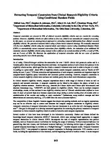
representation of a time annotation on one- and two-dimensional scales is shown in Figure 1: 1D visualization has the disadvantage that it does not allow an unambiguous placement of DI, a problem that can be solved by 2D visualization [23]. Despite this limitation, we will use 1D visualization in the remaining part of this paper for two reasons: First, we found it to be much more intuitive and second, an unambiguous placement of DI is not essential for our purpose. *** Insert Figure 1 here *** By defining three time intervals from which the time annotation’s starting and ending time points and duration may originate, Asbru permits representation of temporal uncertainty. As each time annotation can further define its local reference point, multiple time lines are permitted. To support incomplete temporal information, parameters may be left unrestricted, denoted by "_". Logically, this corresponds to setting the parameter to the respective bound of its interval’s domain, i.e. an unrestricted minDu is set to 0, ESS to −∞, and LFS to ∞. Note that none of the intervals is redundant. Any change in an interval’s parameters has an influence on the time annotation’s characteristics, as long as it stays within the bounds ([ESS-, LSS+], [EFS, LFS+], [minDu-, maxDu+]) given by ([EFS – maxDu, LFS – minDu], [ESS + minDu, LSS + maxDu], [MAX(0, EFS – LSS), LFS – ESS]). As we will describe in section 4.1, a time annotation may be regarded as a temporal constraint network with three variables for Ref, the start and the finish of an event, and the three intervals building distance constraints between them. In this interpretation, the above restriction on the intervals’ bounds corresponds to the properties of a minimal network, which provides the most explicit encoding of the involved constraints [3]. If at least one parameter of SI or FI is defined together with a reference point, we say that a time annotation of a plan element is linked to the time line. This means that the plan element may not start or finish before or after a certain point in time. If only DI is defined, however, the time annotation is completely detached from the time line. The plan element may be executed at any time, as long as its duration stays within the specified limits. 3.2.2
Plan body
In Asbru, a clinical guideline is modeled as a set of hierarchical plans. As indicated by the term hierarchical, each plan may contain any number of subplans within its plan body, which may themselves be decomposed into sub-subplans, and so on. In the remaining part of this paper, such a tree structure of plans, starting from one root plan down to its leaf plans, will be referred to as a plan hierarchy; the term will be used as a synonym for a clinical guideline coded in the Asbru language. Each plan corresponds to a single guideline activity (e.g., the activity weaning is represented as one
- 10 -
to appear in Artificial Intelligence in Medicine, 2002. of several plans within a plan hierarchy for the artificial ventilation of neonates). Note that the root plan of a plan hierarchy constitutes the top-level activity and is usually named after the guideline itself (e.g., plan artificial ventilation of neonates). The control flow within a plan hierarchy is explicitly specified and allows sequential (with defined or undefined order), parallel, cyclic, and arbitrary execution of plans. During run-time, a plan is decomposed into its subplans until a non-decomposable plan – known as action – is found. Actions are executed by the user or by an external call to a computer program. A set of predefined actions exists in order to carry out interaction with the user or to retrieve information from the patient’s medical records. In order to constrain the possible time intervals of its execution, a plan may be associated with a time annotation that defines a temporal scheduling constraint for the plan. The resulting data structure will be termed plan activation (PA) in the remaining part of this paper. The time interval during which a plan is actually executed will be known as its execution interval (EI). Within a PA, a plan may only be associated with one time annotation; disjunctions of several time annotations are not allowed. As an example, the plan activation (GDM-II [[0 WEEKS, 8 WEEKS], [24 WEEKS, _], [18 WEEKS,_], CONCEPTION]) means: "Plan GDM-II for the treatment of gestational diabetes
mellitus type II should be executed in a time interval, starting between 0 and 8 weeks after the conception, finishing no earlier than 24 weeks after the conception, and lasting at least 18 weeks." There are no restrictions on the latest finishing point and the maximum duration. Example 1. A plan hierarchy consisting of 11 PAs in 4 levels. Control flow is specified by 5 different
operators. (P1 [[_,_],[_,390],[50,370],Ref] do-seq-ordered ((P2 [[_,_],[_,_],[70,100],_]), (P3 [[_,_],[_,_],[120,150],_]), (P4 [[_,_],[_,_],[130,160],_]))) (P2 do-parallel ((P5 [[_,_],[_,_],[90,_],_]), (P6 [[40,_],[_,_],[_,_],Ref]))) (P3 do-cyclic ((P7 [[_,_],[_,_],[20,_],_] retry=[10,_] exec=[5,_]))) (P4 do-arbitrary ((P8 [[_,_],[_,_],[120,160],_]), (P9 [[_,_],[_,_],[20,_],_]))) (P8 do-seq-unordered ((P10 [[_,_],[_,_],[90,_],_]), (P11 [[_,_],[_,_],[80,_],_])))
- 11 -
Example 1 shows a plan hierarchy that covers all three kinds of scheduling constraints examined in this paper, namely (1) temporal scheduling constraints, (2) scheduling constraints implied by the guideline’s control flow, (3) scheduling constraints implied by a hierarchical structuring of a guideline: the plan hierarchy consists of eleven plans in four layers, each of which is associated with a specific time annotation and thus constitutes a PA. The execution of plans within the hierarchy is further influenced by five different operators for flow control. The semantics of these operators and the additional parameters of the cyclic operator will be explained in section 4.3.2. The actual guideline actions (such as recommendations to the user) reside in the plan bodies of the leaf plans. As they are not essential for our task, they are omitted in Example 1.
4 Verification of scheduling constraints The PAs within an Asbru plan hierarchy, building a set of temporal scheduling constraints for the involved plans constitute the target of our verification approach. We will show in section 4.1 how our task of verifying PAs can be mapped to a simple temporal problem. In section 4.2 we will then define the properties consistency and minimality, for which PAs are checked in the verification process. In sections 4.3 and 4.4 we will examine how inconsistencies and non-minimalities may arise within a single PA or within a network of several PAs. Asbru’s operator for unordered, sequential execution of plans does not fit into our framework, and will therefore be separately handled in section 4.5. In section 4.6, we will address the problem of multiple time lines within different PAs, which complicates verification.
4.1
Analogy to a simple temporal problem
Our verification task can be mapped to a simple temporal problem: according to Dechter et al., a simple temporal problem (STP) is a temporal constraint satisfaction problem in which all involved (quantitative) constraints consist of a single interval [3]. This is a special case of the general temporal constraint satisfaction problem, where constraints are disjunctions of intervals. The constraint network of an STP can be represented by a directed constraint graph (CG): Nodes represent variables X1, ..., Xn for the time point of the occurrence of certain events, whereas an edge i→j indicates that an interval [aij, bij] for the temporal distance between the two corresponding events is specified, representing the constraint aij ≤ Xj – Xi ≤ bij. Within the constraint network of an STP, no more than one interval per edge is allowed, which means that disjunctions of constraints are ruled out.
- 12 -
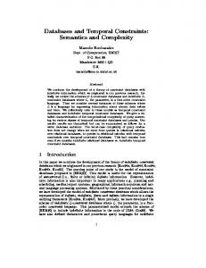
to appear in Artificial Intelligence in Medicine, 2002. Each constraint can equally be expressed by a pair of inequalities Xj – Xi ≤ bij and Xi – Xj ≤ –aij. This constitutes the basis of the directed distance graph (DG), which has the same node set as the CG. Each edge i→j, however, is labeled by a single weight aij representing the linear inequality Xj – Xi ≤ aij. As an example, on the right side of Figure 2 the weight on the edge from P.S to P.F constrains the distance P.F – P.S to be lower or equal to maxDu. A PA with a fully specified time annotation constrains the start, finish and duration of a plan. As it does not allow disjunctions of time annotations, it satisfies the corresponding demand of an STP. In order to represent a PA as the constraint network of an STP, we decompose it into the three nodes Start of Plan (P.S), Finish of Plan (P.F) and Reference Point (Ref). Figure 2 shows the CG and DG corresponding to a PA. *** Insert Figure 2 here ***
4.2
Properties to be checked
We verify the PAs within an Asbru plan hierarchy by checking them for the following two properties: • Consistency We examine whether PAs are consistent with those scheduling constraints within a guideline, which are induced by control flow operators or hierarchical structuring. To cite an example, our goal is to check whether the PAs within a plan hierarchy, such as the one depicted in Example 1, are consistent. The concept of consistency we use is based on the absence of negative cycles within the DG of an STP, as defined by Dechter et al. [3]: We consider a PA to be consistent with respect to its associated time annotation if and only if its DG representation does not contain negative cycles. A negative cycle is defined as a cyclic path within the DG, for which the sum of weights aij (c.f., section 4.1) is negative. In this paper, a PA that is consistent with respect to its associated time annotation will be referred to by the shorter term, consistent PA only. • Minimality We examine whether each PA is minimal with respect to its time annotation. Using the abbreviated version minimal PA in the remaining part of this paper, we consider a PA to be minimal if and only if the constraint network, given by the three intervals of the associated time annotation, is minimal. The concept of minimality of a constraint network is defined the same way as Dechter et al. [3] have done: A constraint network is minimal if it is tighter than any
- 13 -
equivalent constraint network. Two networks are equivalent if they represent the same solution set, which in our case corresponds to two PAs that allow the same set of EIs for their plans. A network T is tighter than a network S if all constraints of T are tighter than the corresponding constraints in S, i.e. constraint Tij is tighter than Sij for all pairs i,j. A constraint Tij, limiting the distance between two variables is tighter than a constraint Sij, if every pair of values allowed by Tij is also allowed by Sij. In other words, a PA is minimal if its time annotation represents the most explicit encoding of the induced constraints. Inconsistencies are treated as errors that have to be cleared by the user. Non-minimalities, however, only represent sub-optimal specifications of PAs that commonly occur within guidelines: In fact, most PAs will be non-minimal when initially defined by the user, as the latter usually does not want to be concerned with checking each PA for minimality. When derived from real-world constraints, PAs may even be voluntarily kept non-minimal. Therefore, they are only indicated to the user; their correction is not enforced.
4.3
Inconsistencies
As the presence of a negative cycle indicates that an STP is inconsistent, we will examine in the sequel how cycles may arise within one PA or within a network of several PAs. For each identified type of cycle we will examine how it may become negative and thereby introduce an inconsistency. We will start by inspecting a single PA for negative cycles in section 4.3.1. In the examination of a network of PAs, we will distinguish three causes of linking PAs: (1) the specification of control flow in section 4.3.2; (2) parent–child relations in section 4.3.3; and (3) links to the time line in section 4.3.4. 4.3.1
Single plan activation
If we take a look at the DG of a single fully specified PA (see right side of Figure 2), we find that cycles are already identifiable here. First we have three cycles, each enclosing two of the three nodes: ESS and LSS build a cycle between Ref and P.S, EFS and LFS between Ref and P.F, and finally minDu and maxDu form a cycle between P.S and P.F. A trivial kind of inconsistency will occur here when at least one of the following inequalities holds: ESS > LSS, EFS > LFS or minDu > maxDu Second, we receive two cycles that span all three nodes of a PA: that comprising ESS, LFS, and minDu, and that comprising LSS, maxDu, and EFS. All other cycles that span all three nodes are
- 14 -
to appear in Artificial Intelligence in Medicine, 2002. concatenations of two two-node cycles and may be correspondingly decomposed. Inconsistencies resulting from the latter two cycles will occur if at least one of the following inequalities holds: minDu > LFS – ESS or EFS – LSS > maxDu Looking for relative positionings of SI and FI that can be excluded a priori as being inconsistent, the latter two inequalities give us the following trivial insight: considering that the minimum value for minDu is 0, the first inequality tells us that an FI, that is in relation before to SI, is always inconsistent. The second leaves any position of SI relative to FI open, as maxDu is unbound on the upper end. 4.3.2
Specification of control flow
As mentioned in section 3.2, the Asbru language provides operators that allow the user to explicitly define the order in which plans are to be executed. We will now examine what kind of constraints between PAs are imposed by the semantics of these operators for flow control. *** Insert Figure 3 here *** Sequential execution of plans with defined order Asbru provides an operator for sequential, ordered execution of plans with common semantics: Every plan, activated as the (i+1)th member of a set of sequential plans with defined order, may not be started before the plan corresponding to the ith member is completed. In other words, a sequential ordered execution of plans P1 and P2 implies the qualitative constraint P1.F ≤ P2.S between the finish of P1 and the start of P2. This translates to the quantitative constraint [0, ∞) between time points P1.F and P2.S [13]. Figure 3 (a) visualizes this circumstance in the CG and DG. The maximum distance of ∞ is omitted in the DG, as it does not represent a constraint. Parallel execution of plans The Asbru operator for parallel execution of plans has the following semantics: Parallel plans have to start concurrently, whereas no restriction is made for their finishing time point. This entails the qualitative constraint P1.S = P2.S between the starting time points of parallel plans P1 and P2, which translates to a maximum (and therefore also minimum) distance of 0 between these points. Figure 3 (b) is a graphical representation of this constraint for two parallel plans. The edges are presented in diagonal orientation to optically distinguish them from parent-child relationships. Arbitrary execution of plans
- 15 -
The operator for arbitrary execution of plans does not impose any constraint on the order: Plans may be executed in parallel, overlapping or sequential fashion. Therefore, the distance between them cannot be restricted in any way. For reasons of completeness, Figure 3 (c) visualizes the unconstrained distance between the start and the finish of two arbitrary executed plans. Cyclic execution of plans The Asbru language offers several ways to specify a repetitive execution of a single plan. All these alternatives are extensions of the following scheme: A regular PA is enhanced by a retry-delay and a lower (minExec) as well as an upper limit (maxExec) for the number of plan executions. The retrydelay is given by an interval that defines the minimum (minDelay) and maximum waiting period (maxDelay) between two plan executions. Figure 3 (d) shows the DG of the cyclic execution of a single plan. The upper graph gives a static view of the cyclic plan, whereas the lower graph shows one particular instance in detail. As the retry-delay and number of plan executions can be defined by the user, they are susceptible to inconsistencies. We mentioned in section 4.3 that a PA is inconsistent if minDu > maxDu. Similarly, a cyclic PA is inconsistent if (minDu ⋅ minExec) + (minDelay ⋅ (minExec – 1)) > (maxDu ⋅ maxExec) + (maxDelay ⋅ (maxExec – 1)). 4.3.3
Parent–child relations
As stated in section 3.2, Asbru organizes guidelines in a tree structure of plans known as a plan hierarchy. A plan hierarchy may consist of several levels, and each non-leaf plan has a parent → child relationship with its subplans on the next lower level. Using the obvious approach of parent– child synchronization, Asbru does not allow child plans to start before their parent or to finish after their parent. For a parent plan P and a child plan C, this entails the qualitative constraints P.S ≤ C.S and C.F ≤ P.F between their starting and finishing time points. This translates to a minimum distance of 0 between P.S and C.S and a minimum distance of 0 between the C.F and P.F [13]. *** Insert Figure 4 here *** Figure 4 (a) visualizes this circumstance in the CG and DG. Clearly, the PAs of plans P and C will be inconsistent if C.minDu > P.maxDu. If we combine the constraints originating from control flow with those originating from parent–child relationships, we receive less obvious possibilities for inconsistencies: Figure 4 (b) depicts a scenario where plan P1 has two child plans P2 and P3, which are executed sequentially in order P2, P3. Plan P2 itself is parent of the cyclic plan P4. The scenario in Figure 4 (b) contains three different cycles. Cycle 1 between P2 and P4, shown in dark, may induce an inconsistency between the PAs of P2 and
- 16 -
to appear in Artificial Intelligence in Medicine, 2002. P4, if P4.[(minDu ⋅ minExec) + (minDelay ⋅ (minExec - 1))] > P2.maxDu. Cycle 2 between P1, P2 and P3, represented in medium gray, may yield an inconsistency if P2.minDu + P3.minDu > P1.maxDu. Cycle 3 is depicted in light gray and circumvents the minimum duration of P2 by passing over P4. It will be inconsistent if P3.minDu + P4.[(minDu ⋅ minExec) + (minDelay ⋅ (minExec - 1))] > P1.maxDu. Note that the third cycle is not rendered obsolete by the other two: The total minimum duration of all instantiations of P4 can be lower than the maximum duration of P2 (hereby avoiding an inconsistency in cycle 1), but higher than the minimum duration of P2 at the same time. Together with the minimum duration of P3, it may then exceed the maximum duration of P1, causing an inconsistency in cycle three. 4.3.4
Links to the time line
We have seen in sections 4.1 and 4.3.1, how links to the time line can create cycles within a single PA. Now we will demonstrate that such cycles may also span several PAs. Depending on the involved control flow operators, different kinds of cycles are possible. Therefore, we will examine in the following for each control flow operator, how links to the time line within the involved PAs may induce inconsistencies: Sequential execution of plans with defined order We assume a set of sequential plans with defined order, where an early executed plan Pm has a link to the time line of the "earliest" type (ESS or EFS defined) and a later executed plan Pn has one of the "latest" type (LSS or LFS defined) with m < n. Then these links form a cycle within the corresponding DG, which further involves the minimum durations of the intermediate plans, the minimum durations of 0 between the finish and the start of neighboring plans and potentially the minimum durations of Pm and Pn. *** Insert Figure 5 here *** We omit cycles in the opposite direction, as they involve the unconstrained maximum distances of ∞ between the finish and the start of consecutive plans. Figure 5 shows the possible scenarios with grayed minimum duration constraints and the conditions for each cycle to become inconsistent. Parallel execution of plans We assume a set of parallel plans including plans Pi and Pj, which have links to the time line of the opposite type, i.e. one of the "earliest" type and the other of the "latest" type. We then distinguish four types of cycles induced by these links. Figure 6 shows the scenarios with grayed duration
- 17 -
constraints and the conditions for each cycle to become inconsistent. *** Insert Figure 6 here *** Arbitrary execution of plans As the minimum and maximum distances in the DG between two arbitrarily executed PAs are +∞, a cycle involving two or more such plans (of the same parent) cannot become negative. Inconsistencies can only originate from cycles that involve the links between a single arbitrarily executed plan and its parent or children plans. Cyclic execution of plans If a cyclic PA defines an SI and/or an FI, these refer to the start of the first execution and/or to the finish of the last execution of the plan. As already shown, the total minimum and maximum durations between the start of the first and the finish of the last executions are (minDu ⋅ minExec) + (minDelay ⋅ (minExec - 1)) and (maxDu ⋅ maxExec) + (maxDelay ⋅ (maxExec - 1)). As we thus treat all executions of a cyclic PA as a whole and its links to the time line can only refer to the first and last executions, only a single PA is involved here. Therefore, a cyclic PA linked to the time line can only be part of a network of PAs through the links to its parent or children plans; it cannot generate a network of PAs itself. Therefore, when examining a network of PAs for inconsistencies, cyclic plans only have to be considered as part of those cycles that include the cyclic plan’s links to its parent and/or children plans. However, each single cyclic plan may itself become inconsistent, as shown in section 4.3.2.
4.4
Non-minimalities
In this section, we will examine how non-minimalities may arise within one PA or within a network of several PAs. Although we do not allow inconsistent PAs within a plan hierarchy, we do not force the user to define minimal PAs during the design of a plan hierarchy. Ensuring manually that each PA is minimal would be annoying for her. Instead, we point out non-minimal PAs to the user during plan verification, and give her the option to adapt it. Providing the minimal variant of a PA as a suggestion on how to modify it does not require extra effort: The algorithm we use for consistency checking is based on the computation of minimal PAs within a plan hierarchy. 4.4.1
Single plan activation
A single PA that is consistent by not containing a negative cycle as described in section 4.3.1, is not
- 18 -
to appear in Artificial Intelligence in Medicine, 2002. necessarily minimal. It will be minimal when it satisfies the following additional demands that can be deduced from the definition of a time annotation’s bounds ([ESS-, LSS+], [EFS-, LFS+], [minDu, maxDu+]), as given in section 3.2. • ESS ≤ EFS and LSS ≤ LFS • MAXIMUM (0, EFS – LSS) ≤ minDu ≤ MINIMUM (EFS – ESS, LFS – LSS) • MAXIMUM (EFS – ESS, LFS – LSS) ≤ maxDu ≤ LFS – ESS The first point allows SI to be in any of the relations {equal, overlaps, meets, before} to FI. Depending on SI and FI, the second and third points yield the bounds for DI. On the left side of Figure 7 (a), a PA that does not satisfy the above demands is shown: One objection to minimality consists in its EFS being smaller than ESS. The PA on the right side of Figure 7 (a) represents an equivalent minimal version of the same PA that satisfies the above demands. We use the 1D representation introduced in Figure 1 here, as it allows a graphical visualization of the difference between non-minimal and minimal PAs. *** Insert Figure 7 here *** 4.4.2
Network of plan activations
Non-minimality of a PA may also be induced by links to other PAs in a common network. The left side of Figure 7 (b) shows a plan hierarchy containing PAs that are rendered non-minimal by two types of scheduling constraints: One is implied by a control flow operator for sequential execution and the other by a parent−child relation.
4.5
Handling Asbru’s operator for unordered, sequential plan execution
The Asbru language includes an operator for sequential execution of plans, where the order in which the plans are executed is not specified. Accordingly, an unordered sequential execution of plans P1 and P2 presumes that P1 is executed either before or after P2. In terms of the DG, this means that there is a minimum distance of 0 either between the finish of P1 and the start of P2, or between the finish of P2 and the start of P1. The disjunctions within the last two sentences already indicate that an unordered, sequential execution of plans exceeds the scope of STPs. It also does not fit into the framework of general temporal constraint satisfaction problems (TCSPs), as defined by Dechter et al. [3]: Although their TCSP framework allows disjunctions within constraints, the latter may only be of the binary type. This means that each disjunct within one disjunction must exclusively refer to the same pair of
- 19 -
variables (e.g., a ≤ Xj – Xi ≤ b ∨ c ≤ Xj – Xi ≤ d). However, the unordered sequential execution of plans P1 and P2 introduces the 4-ary constraint 0 ≤ P2.S – P1.F ≤ ∞ ∨ 0 ≤ P1.S – P2.F ≤ ∞. To incorporate the unordered sequential execution of plans, we need an approach that can handle non-binary constraints, such as the framework proposed by Stergiou and Koubarakis [29]. They consider temporal constraints of the form X1 – Y1 ≤ r1 ∨ …∨ Xn – Yn ≤ rn , where X1, …, Xn, Y1, …, Yn are variables and r1, …, rn are constants. This covers the representation of unordered sequential plans, e.g. for plans P1, P2 and P3 we would define the three constraints (P1.F – P2.S ≤ 0) ∨ (P2.F – P1.S ≤ 0), (P1.F – P3.S ≤ 0) ∨ (P3.F – P1.S ≤ 0) and (P2.F – P3.S ≤ 0) ∨ (P3.F – P2.S ≤ 0). However, the problem of determining the consistency of a set of constraints that includes disjunctions of non-binary constraints is NP hard. Therefore, we choose to apply partial verification for unordered sequential plans only, by checking whether there are any easily identifiable objections to their consistency: • We check whether there is any objection to the assumption that the set of plans can be executed in sequential order at all. This is the case if two or more of the corresponding PAs are overlapping, which means that they force the plans to be executed at least partially in parallel. Whether two PAs are overlapping can be deduced from their parameters LSS and EFS: Overlapping(PA1, PA2) iff ((LSS(PA1) < EFS(PA2)) ∧ (LSS(PA2) < EFS(PA1))) If two or more PAs of a set of unordered sequential plans are overlapping, we will receive an inconsistency (i.e. a negative cycle within their DG), no matter how we arrange them. • The constraint on the EI of a child plan with respect to its parent’s EI (see section 4.3.3) clearly also holds for unordered, sequential plans. The corresponding constraints are inserted in the matrix of weights accordingly (see section 5). • The total minimum durations of a set of unordered, sequential plans must not exceed their parent’s maximum duration. To perform the corresponding check, we can execute an additional verification run, where we treat the set of unordered, sequential plans as ordered, sequential plans, considering only their DIs but ignoring their SIs and FIs.
4.6
Verification with multiple time lines
As we have seen in section 4.3.4, our verification process involves checking whether particular constraints among two or more PAs, which are linked to the time line, are consistent. This purpose is
- 20 -
to appear in Artificial Intelligence in Medicine, 2002. rendered difficult by Asbru’s ability to support multiple time lines within one plan hierarchy: Asbru allows the reference point of a PA to refer to patient-specific time points (e.g., birth, conception, ...). The actual calendar date for such a time point can only be determined during the
execution of a plan, after it has been assigned to a patient. Statically, its relation to another PA’s reference point is a priori unknown, which means that the distance between them is set to (−∞, +∞). This, in due course, can prevent certain "obvious" inconsistencies from being detected: Let us assume that we have to check, in the context of a guideline for the treatment of gestational diabetes, whether plans P1 and P2 can be executed sequentially in order P1, P2, when activated by (P1 [[_,_],[2,_], [_,_],delivery]) and (P2 [[_,2],[_,_],[_,_],conception])
(see upper diagram in Figure 8REFFORMATVERBINDEN). As the unknown distance between the two reference points turns the sum of weights of the induced cycle to +∞, a sequential execution of P1 and P2 is found to be consistent (see lower left diagram in Figure 8). *** Insert Figure 8 here *** In such a case, verification can be optimized if additional knowledge on the relation between the reference points of different PAs is available. Let us assume that we include such knowledge in our checking process, i.e. for the same pregnancy, the event delivery always happens after the event conception. This translates to a constraint of [ε, +∞) on the distance between them, where ε
represents the smallest supported time unit. When using this additional knowledge, a sequential execution of P1 and P2 is found to be inconsistent (see lower right diagram in Figure 8). No additional knowledge is needed when checking PAs with identical reference points, as they are trivially related. The same holds for PAs, whose reference points are specified as time points of the calendar.
5 Verification method Like Dechter et al., we use Floyd-Warshall’s all-pairs-shortest-paths algorithm to detect inconsistencies within a network of PAs: for i,j = 1 to n do dij ← aij; for i = 1 to n do dii ← 0; for k = 1 to n do for i,j = 1 to n do dij ← min(dij, dik + dkj);
- 21 -
Applied to the network’s DG, the algorithm calculates the minimal network represented as a matrix of minimum distances dij in time O(n3), where n is the number of nodes. Inconsistencies (i.e. negative cycles) can simply be detected by examining the sign of the diagonal elements dii within the minimum distance matrix. The matrix of weights aij is set up by inserting the defined constraints originating from the individual PAs, parent-child relations and control flow operators. Instead of the value ∞ for unconstrained distances, we use the constant INF = (n ⋅ MAX(aij)) + 1, as no path can have more than n arcs. The algorithm further permits the identification of non-minimal PAs and provides their minimal versions as a suggestion on how to adapt them. We make use of this feature by pointing out nonminimal PAs to the user during the verification process and leave her the choice of accepting the minimal version, modifying the PA differently or leaving it as it is. An additional benefit of calculating the minimal network is the fact that it may be used to assemble solutions, i.e. assignments to the parameters of all PAs, that are consistent with the network’s constraints in time O(n2). Finding a solution of the network is an essential task for the guideline interpreter to determine the EIs of all plans. *** Insert Table 1 here *** To demonstrate the set-up process of our method, Table 1 (a) shows the matrix of weights aij, after inserting the constraints of plan P2 and its subplans of Example 1 (we use here only this part of the entire plan hierarchy, in order to keep the example simple). The value 701 corresponds to INF. Figure 9 provides an obvious depiction of the weights corresponding to all other values: The value 0 at cells (P5.S, P2.S), (P2.F, P5.F), (P6.S, P2.S), and (P2.F, P6.F) originates from parent-child relations. The value 0 at cells (P5.S, P6.S) and (P6.S, P5.S) originates from the parallel execution of plans P5 and P6. The value –40 at cell (P6.S, Ref) originates from the ESS of P6. All other values originate from the minimum or maximum durations of plans P2 and P5. Table 1 (b) shows the matrix of minimum distances dij, which results from applying FloydWarshall’s algorithm to the matrix of weights in Table 1 (a). It demonstrates that the PAs within P2 and its subplans are consistent, as it does not contain a negative diagonal elements dii. It further shows that none of the three PAs is minimal: For P2 the values of ESS, LSS, EFS and minDu, corresponding to cells (P2.S, Ref), (Ref, P2.S), (P2.F, Ref), and (P2.F, P2.S) can be tightened. For P5 all values except minDu and LFS can be tightened. For P6 all values except ESS and LFS can be tightened.
- 22 -
to appear in Artificial Intelligence in Medicine, 2002.
6 Evaluation of the verification method Four existing clinical guidelines have been represented in the Asbru language so far. These include the following: a guideline for the observation and treatment of gestational diabetes mellitus used at the Stanford Medical School, which is based on the California Diabetes and Pregnancy Program "Sweet Success"; a guideline that supports the artificial ventilation of neonates used at the neonatal intensive care unit of the University of Vienna Medical School [6]; a guideline for the treatment of sinusitis used by general practitioners in the Netherlands [31]; and a guideline for the management of hyperbilirubinemia in newborns, issued by the American Academy of Pediatrics [1]. Although these four guidelines comprise numerous scheduling constraints implied by control flow and hierarchical structuring, PAs are barely utilized. Therefore, they do not represent interesting subjects for an automatic verification of their temporal scheduling constraints. For the demonstration of our approach, we will thus verify the PAs within the fictive guideline shown in Example 1. This guideline is an interesting test case, as it covers all three kinds of scheduling constraints examined in this paper, including several variants thereof, namely (1) temporal scheduling constraints: different variants of incomplete time annotations are used, some of which are linked to the time line; (2) scheduling constraints implied by the guideline’s control flow: the full spectrum of Asbru’s control flow operators is covered; (3) scheduling constraints implied by a hierarchical structuring of a guideline: the plan hierarchy is arranged in four different levels. *** Insert Figure 9 here *** To visualize the different cycles emerging from this guideline, we depict the corresponding DG in Figure 9. It does not include the two unordered sequential plans P10 and P11, as the corresponding constraints on their control flow cannot be represented within a DG. As an XML-DTD (Document Type Definition) exists for the current version of Asbru, in the final implementation of our verifier we intended to employ XML as the import format of Asbru plans. The prototype verifier, which we currently use and present in this paper, is confined to a manual specification of the plan hierarchy within the verifier. Its verification algorithm, however, is based on the method described in section 5. The application contains two text areas, where the left side shows the plan hierarchy to be analyzed and the right side depicts the results of the verification process. *** Insert Figure 10 here *** Figure 10 shows the result of verifying the guideline of Example 1. It tells us that the PAs within the plan hierarchy are inconsistent for two reasons: First, an inconsistent path corresponding to a negative cycle within Figure 9 is present, which involves the minimum durations of plans P4, P7 and
- 23 -
P5, the latest finishing shift of P1, the earliest starting shift of P6, and several links induced by control flow operators and parent-child relations. Second, the total minimum duration of the unordered sequential plans P10 and P11 exceeds the maximum duration of their parent plan P8. *** Insert Figure 11 here *** Figure 11 shows the result of verifying the guideline after the two inconsistencies were cleared by setting the latest finishing shift of plan P1 to 420 and the minimum duration of plan P10 to 70. As described in section 4.4, the verifier provides the minimal version of each PA as a suggestion on how to adapt it.
7 Conclusion Scheduling constraints, expressed either explicitly by control flow operators (e.g., for sequential or parallel execution) or implicitly by a hierarchical modeling, are basic elements of most current formats for the computerized representation of clinical guidelines. Another type of scheduling constraint, which is frequently found in conventional guidelines, is given by temporal specifications (e.g., "determine the newborn’s blood glucose level within 30 minutes after birth", "execute a controlled ventilation for at least 3 hours"). The importance of the latter kind of constraint is reflected by a growing number of integrations within current guideline specification formats. However, like other types of knowledge, temporal scheduling constraints may be used inconsistently within a guideline and may thus be an obstacle for the guideline’s computerization. In this paper we have addressed the problem by presenting an approach for the verification of temporal scheduling constraints within clinical practice guidelines, represented in the Asbru language. The approach is based on the calculation of the minimal temporal network, and serves three purposes: (1) it allows the identification of inconsistent temporal scheduling constraints; (2) it detects non-minimal temporal scheduling constraints and yields suggestions for their representation in an equivalent, but more explicit form; and (3) it can be used by the guideline interpreter to determine feasible EIs for each guideline activity. The computation of the minimal network can be done in O(n3) time for a guideline with n individual activities and therefore constitutes an efficient method for its verification. Efficiency is an issue for us insofar as it allows our verification process to be applied interactively during the design phase of a guideline, e.g. after each definition of a new temporal scheduling constraint, without annoying the user by long answering times.
- 24 -
to appear in Artificial Intelligence in Medicine, 2002. A limitation of our approach consists in its inability to fully verify temporal constraints on the execution of unordered sequential guideline activities. Although we apply several checks that can detect basic types of inconsistencies in this case, a full verification would require a technique that can handle disjunctions of non-binary constraints. Even though suitable approaches for this task have been described in the literature [28, 29], the problem of fully verifying a guideline that includes unordered sequential activities is NP hard. As Asbru is currently the only representation format that considers unordered sequential activities, we chose to integrate them in the verification process only through partial checks. Hereby, the efficiency of our approach is not compromised. Our approach is reusable in two ways: (1) It is applicable for the verification of several guideline representation formats other than Asbru, such as GLIF, EON, PROforma, or DILEMMA / PRESTIGE. This is due to the fact that our approach assumes the existence of certain basic operators for flow control within a guideline representation format (such as sequential, parallel or cyclic execution) and its organization in a hierarchical structure. These concepts are realized in most current approaches [5, 9, 18, 19]. Our considerations on temporal scheduling constraints (originating from Asbru’s PAs in this paper) have to be adapted when reusing our approach for a different representation, according to the expressiveness of the respective format in this area. (2) Our approach can be ported to domains other than guideline-based care for the following reasons: First, the Asbru language is suitable for several areas of planning [15]. Second, our verification method is a domainindependent, general approach for processing temporal constraints [3]. Acknowledgments. The authors thank Michael Balser, Frank van Harmelen, Peter Johnson, Robert Kosara, Wolfgang Reif, Andreas Seyfang, Yuval Shahar, and Annette ten Teije, who contribute to the execution of the project. The project is supported by the "Fonds zur Förderung der wissenschaftlichen Forschung" (Austrian Science Fund), P12797-INF.
References [1]
American Academy of Pediatrics, Practice parameter: management of hyperbilirubinemia in the healthy term newborn., Pediatrics 94 (1994) 558-565.
[2]
J. F. Allen, Maintaining knowledge about temporal intervals, Communications of the ACM 26 (1983) 832-843.
[3]
R. Dechter, I. Meiri and J. Pearl, Temporal constraint networks, Artificial Intelligence 49 (1991) 61-95.
- 25 -
[4]
G. Duftschmid and S. Miksch, Knowledge-based verification of clinical guidelines by detection of anomalies, Artificial Intelligence in Medicine 22 (2001) 23-41.
[5]
J. Fox, N. Johns and A. Rahmanzadeh, Disseminating medical knowledge: the PROforma approach, Artificial Intelligence in Medicine 14 (1998) 157-181.
[6]
JP. Goldsmith and EH. Karotkin, Assisted ventilation of neonates (Saunders, Philadelphia, 1993).
[7]
C. Gordon, I. Herbert and P. Johnson, Knowledge representation and clinical practice guidelines: the DILEMMA and PRESTIGE projects, in: Brender-J, Christensen-J, Scherrer-JR and McNair-P, eds., Proceedings of Medical Informatics Europe 96; Copenhagen, Denmark (R. Brompton Hospital London UK. Medical Informatics Europe '96: Human Facets in Information Technologies. IOS Press Amsterdam Netherlands, 1996).
[8]
A. Guarnero, M. Marzuoli, G. Molino, P. Terenziani, M. Torchio and K. Vanni, Contextual and temporal clinical guidelines, in: Proceedings of the AMIA-98 Annual Symposium (1998) 683-687.
[9]
S. Herbert, C. Gordon, A. Jackson-Smale and Salis Renaud, Protocols for clinical care, Computer Methods and Programs in Biomedicine 48 (1995) 21-26.
[10] G. Hripcsak, Writing Arden Syntax medical logic modules, Computers in Biology and Medicine 24 (1994) 331-363. [11] H. A. Kautz and P. B. Ladkin, Integrating metric and qualitative temporal reasoning, in: Proceedings 9th National Conference on Artificial Intelligence (AAAI-91) (AT&T Bell Labs. Murray Hill NJ USA. AAAI Press Menlo Park CA USA, 1991). [12] C. McDonald and J. Overhage, Guidelines you can follow and trust: An ideal and an example, Journal of the American Medical Association (JAMA) 271 (1994) 872-873. [13] I. Meiri, Combining qualitative and quantitative constraints in temporal reasoning, Artificial Intelligence 87 (1996) 343-385. [14] S. Miksch, Plan management in the medical domain, AI Communications 12 (1999) 209-235. [15] S. Miksch, Y. Shahar and P. Johnson, Asbru: A task-specific, intention-based, and timeoriented language for representing skeletal plans, in: Proceedings of the 7th Workshop on Knowledge Engineering: Methods & Languages (KEML-97), Milton Keynes, UK (1997). [16] D.W. Miller, Jr, S.J. Frawley and P.L. Miller, Using semantic constraints to help verify the
- 26 -
to appear in Artificial Intelligence in Medicine, 2002. completeness of a computer-based clinical guideline for childhood immunization, Computer Methods and Programs in Biomedicine 58 (1999) 267-280. [17] M. Musen, J. Rohn, L. Fagan and E. Shortliffe, Knowledge engineering for a clinical trial advice system: uncovering errors in protocol specification, Bulletin du Cancer 74 (1987) 291296. [18] M. Musen, S. Tu, A. Das and Y. Shahar, EON: A component-based approach to automation of protocol-directed therapy, Journal of the American Medical Informatics Association (JAMIA) (1996) 367-388. [19] L. Ohno-Machado, J. Gennari, S. Murphy, N. Jain, S. Tu, D. Oliver, E. Pattison-Gordon, R. Greenes, E. Shortliffe and G. Barnett, The GuideLine Interchange Format: A model for representing guidelines, Journal of the American Medical Association (JAMA) 5 (1998) 357372. [20] E. Pattison-Gordon, J. Cimino, G. Hripcsak, S. Tu, J. Gennari, N. Jain and R. Greenes, Requirements of a sharable guideline representation for computer applications. Stanford Technical Report SMI-96-0628, Stanford University, 1996. [21] M. Peleg, A. A. Boxwala, O. Ogunyemi, Q. Zeng, S. Tu, R. Lacson, E. Bernstam, N. Ash, P. Mork, L. Ohno-Machado, E. H. Shortliffe and R. A. Greenes, GLIF3: the evolution of a guideline representation format, in: Proceedings of the AMIA-2000 Annual Symposium; Los Angeles, CA (2000) 645-649. [22] S. Quaglini, R. Saracco, M. Stefanelli and C. Fassino, Supporting tools for guideline development and dissemination, in: Proceedings of the 6th Conference on Artificial Intelligence in Medicine Europe (AIME) (1997) 39-50. [23] J.F. Rit, Propagating temporal constraints for scheduling, in: Proceedings of the 5th National Conference on Artificial Intelligence (AAAI-86); Los Altos, CA (Morgan Kaufmann, 1986) 383-388. [24] Y. Shahar, S. Miksch and P. Johnson, The Asgaard project: A task-specific framework for the application and critiquing of time-oriented clinical guidelines, Artificial Intelligence in Medicine 14 (1998) 29-51. [25] E. Sherman, G. Hripcsak, J. Starren, R. Jender and P. Clayton, Using intermediate states to improve the ability of the Arden Syntax to implement care plans and reuse knowledge, in: Proceedings of the Annual Symposium on Computer Applications in Medical Care (SCAMC-
- 27 -
95) (1995) 238-242. [26] R. Shiffman, Representation of clinical practice guidelines in conventional and augmented decision tables, Journal of the American Medical Informatics Association (JAMIA) 4 (1997) 382-393. [27] R. Shiffman and R. Greenes, Improving clinical guidelines with logic and decision-table techniques, Medical Decision Making 14 (1994) 245-254. [28] S. Staab, On non-binary temporal relations, in: Prade-H, ed. Proceedings of the 13th European Conference on Artificial Intelligence (ECAI 98) (Comput. Linguistics Lab. Freiburg Univ. Germany. Wiley Chichester UK, 1998). [29] K. Stergiou and M. Koubarakis, Backtracking algorithms for disjunctions of temporal constraints, Artificial Intelligence 120 (2000) 81-117. [30] J. Stillman, R. Arthur and A. Deitsch, Tachyon: A constraint-based temporal model and its implementation, SIGART Bulletin 4 (1993). [31] S. Thomas, R.M.M. Geijer, J.R. van der Laan and Tj. Wiersma, NHG-Standaarden voor de huisarts II (Productie Wetenschappelijke uitgeverij Bunge, Utrecht, 1996). [32] W. Tierney, J. Overhage, B. Takesue, L. Harris, M. Murray, D. Vargo and C. McDonald, Computerizing guidelines to improve care and patient outcomes: the example of heart failure, Journal of the American Medical Informatics Association (JAMIA) 2 (1995) 316-322. [33] S. Vere, Planning in time: Windows and durations for activities and goals, IEEE Transactions on PAMI 5 (1983) 246-267. [34] M. Vilain and H. Kautz, Constraint propagation algorithms for temporal reasoning, in: Proceedings AAAI-86: Fifth National Conference on Artificial Intelligence; Univ (BBN Labs. Cambridge MA USA. American Assoc. Artificial Intelligence Menlo Park CA USA, 1986) 377-382.
- 28 -
to appear in Artificial Intelligence in Medicine, 2002.
finish
time
LFS
maxDu
7 minDu
EFS
maxDu minDu Ref 0 1
ESS 2
LSS EFS 3 4
5
6
LFS
1
7 8 9 10 11 time Figure 1
- 29 -
Ref
1 1 ESS
LSS
start
Ref [ESS,LSS] P.S
Ref [EFS,LFS]
[minDu,maxDu]
−ESS
P.F
P.S
Figure 2
- 30 -
LSS
−EFS maxDu
−minDu
LFS P.F
to appear in Artificial Intelligence in Medicine, 2002. (a)
P1.F
P2.S
[0,∞)
P1.S
(b)
0
P1.F
≈
P1.S
[0,0]
0
≈
0
P2.S
(c)
P1.F
P2.S
(−∞,+∞)
P2.S
P2.S
+∞ +∞
P1.F
≈
P2.S
(maxDu ⋅ maxExec) + (maxDelay ⋅ (maxExec − 1)) P1.S
P1.F − (minDu ⋅ minExec) − (minDelay ⋅ (minExec − 1))
(d)
maxDelay p1(1).S
p1(1).F
p1(2).S −minDelay
Figure 3
- 31 -
...
maxDelay −minDelay
p1(n).S
p1(n).F
P.S
maxDu
[minDu, maxDu]
P.F
P.S
P.F -minDu
(a)
[0,∞) C.S
[0,∞)
≈
0
0 maxDu
[minDu, maxDu]
C.F
C.S
C.F -minDu
maxDu
P1.S
P1.F
Cycle 2 0 seq-ordered
(b)
−minDu
P2.S 0
cyclical
0
P4.S
maxDu
Cycle 1
P2.F 0
−(minDu ⋅ minExec) − P4.F (minDelay ⋅ (minExec − 1))
Figure 4
- 32 -
0
P3.S
Cycle 3
−minDu
P3.F
to appear in Artificial Intelligence in Medicine, 2002. −minDu
Pm.S
0
Pm.F
−ESS
...
0
−minDu
Pn.S
Pn.F
LFS
Ref
−EFS
n
−EFS
...
0
Pn.S
LSS
Ref
i = m+1
−minDu
Pn.S
Pn.F
Pm.S
LFS
Ref
0
Inconsistent, if: Pm.EFS+∑ Pi.minDu > Pn.LSS
i=m
0
...
n-1
Inconsistent, if: Pm.ESS+∑ Pi.minDu > Pn.LFS
Pm.F
0
Pm.F
−minDu
0
Pm.F
−ESS
n
...
Ref
0
Pn.S
LSS
n-1
Inconsistent, if: Pm.EFS+∑ Pi.minDu > Pn.LFS
Inconsistent, if: Pm.ESS+∑ Pi.minDu > Pn.LSS
i=m+1
i=m
Figure 5
- 33 -
maxDu
Pi.S
maxDu
Pi.S
Pi.F
−EFS 0
Pj.S
0
Pj.F
Pj.S
Pi.F −minDu
LSS
−EFS Pj.F LFS
Ref
Inconsistent if:
Pi.EFS – Pi.maxDu > Pj.LSS
Pi.S
Ref
Inconsistent if: Pi.EFS – Pi.maxDu > Pj.LFS – Pj.minDu
Pi.S
Pi.F
Pi.F
−ESS 0
Pj.S
−ESS 0
Pj.F LSS
Pi.ESS > Pj.LSS
Pj.F LFS
Ref
Inconsistent if:
Pj.S
−minDu
Ref
Inconsistent if: Pi.ESS > Pj.LFS – Pj.minDu
Figure 6
- 34 -
to appear in Artificial Intelligence in Medicine, 2002. (P [[1,6],[0,7],[2,_],0])
(P [[1,5],[3,7],[2,6],0])
maxDu
maxDu
minDu
(a)
minDu
EFS
LFS
ESS 0
EFS
LSS
1
2
3
4
5
ESS
6
7
0
1
LSS 2
Non-minimal
(b)
EFS1
ESS3 ESS2 0
1
LSS2 2
4
LFS1
5
6
ESS1 LSS1
LFS2 5
4
7
(P1 [[1,2],[8,9],[6,7],0] do-seq-ordered( (P2 [[1,3],[4,6],[1,4],0]), (P3 [[4,7],[8,9],[1,5],0]))) EFS1 LFS1
LSS3 EFS3 LFS3
EFS2 3
3
Minimal
(P1 [[1,2],[6,9],[4,7],0] do-seq-ordered( (P2 [[0,3],[4,6],[1,4],0]), (P3 [[3,7],[8,9],[1,6],0]))) ESS1 LSS1
LFS
6
7
8 9
Non-minimal
0
ESS3
LSS3
ESS2 LSS2 EFS2
LFS2
1
2
3
4
5
Minimal
Figure 7
- 35 -
6
EFS3 LFS3
7
8 9
delivery
conception
-2 P1.S
2 P1.F
0
P2.S
P2.F
Additional knowledge: "conception < delivery"
No additional knowledge ∞
delivery
conception
-ε
delivery
∞ -2 P1.S
2 P1.F
0
conception
∞
P2.S
-2 P2.F
P1.S
Figure 8
- 36 -
2 P1.F
0
P2.S
P2.F
to appear in Artificial Intelligence in Medicine, 2002. 370 P1.S
P1.F -50
0
0 100
150
0
P2.S
P2.F -70
P3.F
P4.S
-120 0
0
0
P5.S
P5.F
P7.S
P7.F
-90
P4.F -130
0
0
160
0
P3.S
0
0
P9.S
P9.F
-140
0 160 P6.S
P8.S
P6.F
P8.F -120
-40
Ref
-20 390
Figure 9
- 37 -
Figure 10
- 38 -
to appear in Artificial Intelligence in Medicine, 2002.
Figure 11
- 39 -
(a)
(b)
P2.S P2.F P5.S P5.F P6.S P6.F Ref P2.S P2.F P5.S P5.F P6.S P6.F Ref
P2.S 0 -70 0 701 0 701 701 0 -90 0 -90 0 611 611
P2.F 100 0 701 701 701 701 701 100 0 100 10 100 701 701
P5.S 701 701 0 -90 0 701 701 10 -90 0 -90 0 611 611
Table 1
- 40 -
P5.F 701 0 701 0 701 701 701 100 0 100 0 100 701 701
P6.S 701 701 0 701 0 701 701 10 -90 0 -90 0 611 611
P6.F 701 0 701 701 701 0 701 100 0 100 10 100 0 701
Ref 701 701 701 701 -40 701 0 -30 -130 -40 -130 -40 571 0
to appear in Artificial Intelligence in Medicine, 2002. Figure 1. One-dimensional (left) and two-dimensional (right) graphical representation of time annotation [[2, 5], [6, 11], [2, 7], 0]. In 1D visualization, the duration bars must be considered to be "floating" above SI and FI; their position depicted here is only one possible scenario. In 2D visualization, the time annotation is represented as a shaded polygon, which also allows an unambiguous depiction of DI. Figure 2. Constraint graph (left) and distance graph (right) of plan activation (P [[ESS, LSS], [EFS, LFS], [minDu, maxDu], Ref]). Figure 3. Constraint implied by (a) sequential, ordered execution of plans P1 and P2; (b) parallel execution of plans P1 and P2; (c) arbitrary execution of plans P1 and P2. (d) Static view of the cyclic plan P1 with instance p1 below. Instance p1 is executed n times, where minExec ≤ n ≤ maxExec. Within p1, minimum and maximum durations are represented as dashed edges. Figure 4. (a) Constraints between parent plan P and child plan C, shown as vertical edges. The gray horizontal edges represent the duration constraints. They are charted to make cycles obvious. (b) Cycles involving parent-child relations and the control flow. Figure 5. Inconsistent cycles introduced by sequential plans with defined order linked to the time line. Figure 6. Inconsistent cycles introduced by parallel plans linked to the time line. Figure 7. Non-minimal (left side) and minimal (right side) versions of (a) two equivalent single PAs; (b) two equivalent networks of PAs. DIs are omitted. Figure 8. Within a guideline for treating gestational diabetes, it is checked whether plans P1 and P2 may
be
executed
sequentially
[[_,_],[2,_],[_,_],delivery])
and
in (P2
order
P1,
P2,
when
activated
[[_,2],[_,_],[_,_],conception]).
by
(P1
Without additional
knowledge, this scenario is found to be consistent. When the additional knowledge "conception < delivery"
is included, the scenario is found to be inconsistent.
Figure 9. DG of the plan hierarchy, shown in Example 1. Unconstrained durations are shown in gray. Figure 10. Result of verifying the plan hierarchy shown in Example 1. Figure 11. Result of verifying the corrected plan hierarchy. Table 1. Matrix of (a) weights aij; (b) minimum distances dij; for plan P2 and subplans of Example 1. Compare with the corresponding part of DG in Figure 9.
- 41 -