pre(i) â {j âI| j âi = max{hâi | h â I}}. Local lookup at node n is a ...... Note that bnd(β,γ) is defined iff β and γ have finite support and that bnd(β,γ) = 0 iff spt(β) ...
Verifying a Structured Peer-to-peer Overlay Network: The Static Case? EPFL Technical Report IC/2004/76 Johannes Borgstr¨ om1 , Uwe Nestmann1 , Luc Onana23 , and Dilian Gurov23 1
2
School of Computer and Communication Sciences, EPFL, Switzerland Department of Microelectronics and Information Technology, KTH, Sweden 3 SICS, Sweden
Abstract. Structured peer-to-peer overlay networks are a class of algorithms that provide efficient message routing for distributed applications using a sparsely connected communication network. In this paper, we formally verify a typical application running on a fixed set of nodes. This work is the foundation for studies of a more dynamic system. We identify a value and expression language for a value-passing CCS that allows us to formally model a distributed hash table implemented over a static DKS overlay network. We then provide a specification of the lookup operation in the same language, allowing us to formally verify the correctness of the system in terms of observational equivalence between implementation and specification. For the proof, we employ an abstract notation for reachable states that allows us to work conveniently up to structural congruence, thus drastically reducing the number and shape of states to consider. The structure and techniques of the correctness proof are reusable for other overlay networks.
1
Introduction
In recent years, decentralised structured peer-to-peer (p2p) overlay networks [OEBH03,SMK+ 01,RD01,RFH+ 01] have emerged as a suitable infrastructure for scalable and robust Internet applications. However, to our knowledge, no such system has been formally verified. One commonly studied application is a distributed hash table (DHT), which usually supports at least two operations: the insertion of a (key,value)-pair and the lookup of the value associated to a given key. For a large p2p system (millions of nodes), careful design is needed to ensure the correctness and efficiency of these operations, both in the number of messages sent and the expected delay, counted in message hops. Moreover, the sheer number of nodes requires a sparse (but adaptable) overlay network. ?
Short version in the Post-Conference Proceedings of Global Computing 2004, c Springer-Verlag). Supported by the EU-project IST-2001-33234 PEPITO LNCS ( (http://www.sics.se/pepito), part of the FET-initiative Global Computing.
1
The DKS system In the context of the EU-project PEPITO, one of the authors is developing a decentralised structured peer-to-peer overlay network called DKS (named after the routing principle distributed k-ary search), of which the preliminary design can be found in [OEBH03]. DKS builds upon the idea of relative division [OGEA+ 03] of the virtual space, which makes each participant the root of a virtual spanning tree of logarithmic depth in the number of nodes. In addition to key-based routing to a single node, which allows implementation of the DHT interface mentioned above, the DKS system also offers key-based routing either to all nodes in the system or to the members of a multicast group. The basic technique used for maintaining the overlay network, correction-onuse, significantly reduces the bandwidth consumption compared to its earlier relatives such as Chord [SMK+ 01], Pastry [RD01] and Can [RFH+ 01]. Given these features, we consider the DKS system as a good candidate infrastructure for building novel large-scale and robust Internet applications in which participating nodes share computing resources as equals.
Verification approach In this paper, we present the first results of our ongoing efforts to formally verify DHT algorithms. We initially focus on static versions of the DKS system: (1) they comprise a fixed number of participating nodes; (2) each node has access to perfectly accurate routing information. As a matter of fact, already for static systems formal arguments about their correctness turn out to be non-trivial. We consider the correctness of the lookup operation, because this operation is the most important one of a hash table: under all circumstances, the data stored in a hash table must be properly returned when asked for. (The insert operation is simpler to verify: the routing is the same as for lookup, but no reply to the client is required.) We analyse the correctness of lookup by following a tradition in process algebra, according to which a reactive system may be formulated in two ways. Assuming a suitably expressive process calculus at our disposal, we may on the one hand specify the DHT as a very simple purely sequential monolithic process, where every (lookup) request immediately triggers the proper answer by the system. On the other hand, we may implement the DHT as a composition of concurrent processes—one process per node—where client requests trigger internal messages that are routed between the nodes according to the DKS algorithm. The process algebra tradition says that if we cannot distinguish—with respect to some sensible notion of equivalence—between the specification and the implementation regarded as black-boxes from a client’s point of view, then the implementation is correct with respect to the specification. 2
Contributions While the verification follows the general approach mentioned above, we find the following individual contributions worth mentioning explicitly. 1. We identify an appropriate expression and value language to describe the virtual identifier space, routing tables, and operations on them. 2. We fix an asynchronous value-passing process calculus orthogonal to this value language and give an operational semantics for it. 3. We model both a specification and an implementation of a static DKS-based DHT in this setting. 4. We formally prove their equivalence using weak bisimulation. In detail: – We formalise transition graphs up to structural congruence. – We develop a suitable proof technique for weak bisimulation. – We design an abstract high-level notation for states that allows us to succinctly capture the transition graphs of both the implementation and the specification up to structural congruence. – We establish functions that concisely relate the various states of specification and implementation. – We show normalisation of all reachable states of the implementation in order to establish the sought bisimulation. Paper Overview In Section 2 we provide a brief description of the DKS lookup algorithm, and identify the data types and functions used therein. In Section 3, we introduce a process calculus that is suitable for the description of DHT algorithms. More precisely, we may both specify and implement a DKS-based DHT in this calculus, as we do in Section 4. Finally, in Section 5 we formally prove that DKS allows to correctly implement the lookup function of DHTs by establishing a bisimulation containing the given specification and implementation. Related Work To our knowledge, no peer-to-peer overlay network has yet been formally verified. That said, papers describing such algorithms often include pseudo-formal reasoning to support correctness and performance claims. Previous work in using process calculi to verify non-trivial distributed algorithms includes, e.g., the two-phase commit protocol [BH00], a sliding-window protocol [FGP+ 04] and a fault-tolerant consensus protocol [NFM03]. However, in these algorithms, in contrast to overlay networks, each process communicates directly with every other process. Other formal approaches, for instance I/O-automata [LT98] have been used to verify traditional (i.e., logically fully connected) distributed systems; we are not aware, though, of any p2p-examples. 3
Future Work Peer-to-peer algorithms in general are likely to operate in environments with high dynamism, i.e., frequent joins, departures and failures of participating nodes. This case gives us increased complexity in three different dimensions: a more expressive model, bigger algorithms and more complex invariants. To cope with dynamism, structured peer-to-peer overlay networks are designed to be stabilising. That is, if ever the dynamism within the system ceases, the system should converge to a legitimate configuration. Proving, formally, that such a property is satisfied by a given system is a challenge that we are currently addressing in our effort to verify peer-to-peer algorithms. The work present in this paper is a necessary foundation for the more challenging task of formal verification of the DKS system in a dynamic environment. Conclusions The use of process calculi lets us verify executable formal models of protocols, syntactically close to their descriptions in pseudo-code. We demonstrate this by verifying the DKS lookup algorithm. Our choice to work with a reasonably standard process calculus, rather than the pseudo-code that these algorithms are expressed in, made it only slightly harder to ensure that the model corresponded to the actual algorithm but let us use well-known proof techniques, reducing the total amount of work. Other overlay networks, like the above-mentioned relatives of DKS, would require changes to the expression language of the calculus as well as the details of the correspondence proof; however, we strongly conjecture that the structure of the proof would remain the same.
2
DKS
In this section we briefly describe the DKS system, focusing on the lookup algorithm. More information about the DKS system can be found for instance in [OEBH03,OGEA+ 03]. For the design of the DKS system, we model a distributed system as a set of processes linked together through a communication network. Processes communicate by message passing and a process reacts upon receipt of a message; i.e., this is an event-driven model. The communication network is assumed to be (i) connected, each process can send a message directly to any other process in the system; (ii) asynchronous, the time taken by the communication network to forward a message to its destination can be arbitrarily long; (iii) reliable, messages are neither lost nor duplicated. 2.1
The virtual identifier space
For DKS, as for other structured peer-to-peer overlay networks [SMK+ 01,RD01], participating nodes are uniquely identified by identifiers from a set called identifier space. As in Chord and Pastry, the identifier space for DKS is a ring of size 4
N that we identify with ZN , where we write Zn for {0, 1, · · · , n − 1}. To model the ring structure, we let ⊕ and be addition and subtraction modulo N , with the convention that the results of modular arithmetic are always non-negative and strictly less than the modulus. For simplicity, it is assumed that N = k d for k > 1, d > 1, where k will be the branching factor of the search tree. We work with a static system, with a fixed set of participating nodes I ⊆ ZN with |I| > 1.
2.2
Assignment of key-value pairs to nodes
As part of the specification of a DHT, we assume that data items to be stored into and retrieved from the system are pairs (key, val ) ∈ N × N where the keys are assumed to be unique. We model the data items currently in the system as a partial function data : N * N. Using some arbitrary hashing function, H : N → ZN , the key of a data item is hashed to obtain a key identifier H(key) for the pair (key, val ). In DKS (as well as in Chord), a data item (key, val) is stored at the first node succeeding H(key). That node is called the successor of H(key), and is defined as suc(i) ∈ {j ∈ I | j i = min{h i | h ∈ I}}. Note that suc(·) is well-defined since h i = j i iff h j = 0. Dually, the (strict) predecessor of a node i ∈ I is pre(i) ∈ {j ∈ I | j i = max{h i | h ∈ I}}. Local lookup at node n is a partial function datan (j) := data(j) if suc(j) = n, i.e., returning the value data(j) associated to a key j only on the node n responsible for the item (key, val).
2.3
Routing tables
The DKS system is built in a way that allows any node to reach any other node in at most logk (N ) hops under normal system operation. To achieve this, the principle of relative division of the space [OGEA+ 03] is used to embed, at each point of the identifier space, a complete virtual k-ary tree of height d = logk (N ). We let L := {1, 2, · · · , d} be the levels of this tree, where 1 is the top level (the root). At a level l ∈ L, a node n has a view V l of the identifier space. The view V l consists of k equal parts, denoted Iil , 0 ≤ i ≤ k − 1, and defined below level by level. 1 At level 1: V 1 = I01 ] I11 ] I21 ] · · · ] Ik−1 , where I01 = [x10 , x11 ), I11 = [x11 , x12 ), N 1 1 1 1 · · · , Ik−1 = [xk−1 , x0 ), xi = n ⊕ i k , for 0 ≤ i ≤ k − 1. l , where I0l = [xl0 , xl1 ), At level 2 ≤ l ≤ d: V l = I0l ] I1l ] I2l ] · · · ] Ik−1 l−1 N l l l l l = [x1 , x2 ), · · · , Ik−1 = [xk−1 , x1 ), xi = n ⊕ i kl , for 0 ≤ i ≤ k − 1. To construct the routing table, denoted Rtn , of an arbitrary node n of a DKS system we take for each level l ∈ L and each interval i at level l a pointer to the successor of xli , as defined above.
I1l
5
Level Interval Responsible Level 1 [0, 4) 0 2 [4, 8) 5 [8, 12) 10 [12, 0) 13
Interval Responsible [0, 1) 0 [1, 2) 2 [2, 3) 2 [3, 4) 5
0 2 13
5 10 Fig. 1. Routing table for node 0.
Routing table example. As an example, consider an identifier space of size N = 42 , i.e., d = 2 and k = 4. Assume that the nodes in the system are I := {0, 2, 5, 10, 13}. In this case, using the principle described above for building routing table in DKS, we have that node 0 has the routing table in Figure 1. Formally, the routing tables of the nodes are partial functions � � � ��� N (j n)k l Rtn (j, l) := suc n ⊕ if j n < k d+1−l and l ≤ d, kl N where Rtn (j, l) is the node responsible for the interval containing j on level l according to node n. We also define the lookup level for an identifier at a given node as lvln (j) := d − blogk (j n)c, and let lookup in the routing table be Rtn (j) := Rtn (j, lvln (j)), which is defined for all n, j. 2.4
Lookup in a static DKS
The specification of lookup is common to all DHTs: A lookup for a key key at a node n should simply return the associated data value (if any) to the user on node n. Moreover, the system should always be available for new requests, and the responses may be returned in any order. In DKS, the lookup can be done either iteratively, transitively or recursively. These are well-known strategies for resolving names in distributed systems [Gos91]. In this paper, we present a simplified version of the recursive algorithm of DKS. Briefly and informally, the recursive lookup in the DKS system goes as follows. When a DKS node n receives a request for a key key from its user, u, node 6
n checks if the virtual identifier associated to key is between pre(n) and n. If so, node n performs a local lookup and returns the value associated to key to the user. Otherwise, node n starts forwarding the request, such that it descends through the virtual k-ary tree associated with node n until the unique node z such that H(key) is between pre(z) and z is reached. We call z the manager of key. When the manager of key is reached, it does a local lookup to determine the value associated with key. This value is returned, back-tracing the path taken by the request. In order to do this, a stack is embedded in each internal request message, such that at each step of the forwarding process, the node n0 handling the message pushes itself onto the stack. The manager z then starts a “forwarding” of internal response messages towards the origin of the request. Each such message carries the result of the lookup as well as the stack. When a node n receives an internal response message, node n checks if the stack attached to the message is empty. If not, the head of the stack determines the next step in the “backwarding” of the message towards its origin. If the stack is empty, then n was the origin of the lookup. Then node n returns the result of the response to its user, u. The back-tracing makes the response follow a “trusted path”, to route around possible link failures, e.g., between the manager of the key and the originator of the lookup. The stack also provides some fault-tolerance: If the node at the head of the stack is no longer reachable, the nodes below can be used to return the message. A formal model of this lookup algorithm can be found in Section 4, using the process calculus defined in Section 3.
3
Language
We use a variant of value-passing CCS [Mil89,Ing94] to implement the DKS system described above. To separate unrelated features and allow for a simple adaptation to the verification of other algorithms, we clearly distinguish three orthogonal aspects of the calculus. 3.1
Syntax
Values and expressions The values V are integers, lists in nil [ ] and cons v1 :: v2 format and the “undefined value” ⊥. The expressions E contain some standard operations on values, plus common DHT functions and DKS-specific functions seen in Section 2. We extend the domain and codomain of F ∈ {data, lvlv , datav , Rtv | v ∈ I} to V by letting F (v) := ⊥ for the values v on which F was previously undefined. We extend the domain of H to V by letting H take arbitrary values in ZN for values not in N. Expressions are evaluated using the function J·K : E → V. For boolean checks B, we have the matching construct e1 = e2 and an interval check e1 ∈ (e2 , e3 ] modulo N . Boolean checks are evaluated using the predicate 7
eb (·). Values and boolean checks are defined in Table 1, both J·K and eb (·) are defined in Table 3.2. We do not use a typed value language, although the equivalence result obtained in Section 5.2 intuitively implies that the implementation is “as well-typed as” the specification. We use tuples e˜ of expressions (and other terms), where e˜ := e1 , . . . , e|˜e| that may be empty, i.e., |˜ e| = 0. To evaluate a tuple of expressions, we write J˜ eK for the tuple of values Je1 K, . . . , Je|˜e| K. As a more compact representation of lists of values, we write [u˜ v ] for u :: [˜ v ], and also define last([v1 , v2 , · · · , vn ]) := vn if n > 0. Control Flow Structures We use the standard if φ then P else Q and a switch statement case e of {j 7→ Pj | j ∈ S} for a more compact representation of nested comparisons of the same value. In all case statements, we require S ⊂ V to be finite. To gain a closer correspondence to the method-oriented style usually used when presenting distributed algorithms, we work with defining equations for process constants Ah˜ ei rather than recursive definitions embedded in the process terms. If a process constant A does not take any parameters, we write A for both Ahi and A(). Parallel language We use a polyadic value-passing CCS, with asynchronous output and input-guarded choice. We assume that the set of names a, b ∈ N and the set of variables x, y ∈ W are disjoint and infinite. The syntax of the calculus can be found in Table 1. P j∈J Gj for 0 +Gj0 + Gj1 + · · · + Gjn and Q As an abbreviation we write P for 0 | P | P | · · · | P , where J = {ji | 0 ≤ i ≤ n} (J may be ∅). j j j j 0 1 n j∈J 3.2
Semantics
The set of actions A 3 µ is defined as µ ::= τ | a v˜ | a v˜. The channel of an action, ch : A → N ∪ {⊥}, is defined as ch(τ ) := ⊥, ch(a v˜) := a and ch(a v˜) := a. The variables x ˜ are bound in a(˜ x).P . Substitution of the values v˜ for the variables x ˜ in process P is written P [v1/x1 , . . . ,vn /xn ] and performed recursively on the non-bound instances of x ˜ in P. We use a standard labelled structural operational semantics with early input (see Table 2). To compute the values to be transmitted, instantiate process constants and evaluate if and case statements we use an auxiliary reduction relation > (see Table 2).
8
u, v ::= 0, 1, 2, · · · e
::= | | |
|
[]
|
⊥
|
values V
u :: u
u | x head(e) | tail(e) | e :: e data(e) | H(e) lvlv (e) | datav (e) | Rtv (e)
expressions E (lists) (global) (local)
φ, ψ ::= e = e | e ∈ (e, e ]
boolean tests B (interval check)
G
input-guarded sums G (input prefix) (choice)
::= 0 | a(˜ x).P | G+G
P, Q ::= | | | | | |
processes P (asynchronous output) (parallel) (restriction) (process constant) (if statement) (case statement)
G ah˜ ei P |P (P ) \ a Ah˜ ei if φ then P else P case e of {j 7→ Pj | j ∈ S} Table 1. Syntax
Structural congruence is a standard notion of equivalence (cf. [MPW92]) that identifies process terms based on their syntactic structure. In a value-passing language, it often includes simplifications resulting from the evaluation of “toplevel” expressions (cf. [AG99]). In our calculus, top-level evaluation is treated by the reduction relation >, which is contained in the structural congruence. Definition 1 (Structural congruence). Structural congruence ≡ is the least equivalence relation on P containing > and satisfying commutative monoid laws for (P, | , 0) and (G, +, 0) and the following inference rules. S-par
P1 ≡ P10 P1 | P2 ≡ P10 | P2
S-sum
S-res
G1 ≡ G01 G1 + G2 ≡ G01 + G2
P ≡ P0 (P ) \ a ≡ (P 0 ) \ a
Depending on the actual structural congruence rules at hand it is well known, and is straightforward but tedious to show, that structurally congruent processes give rise to the “same” transitions (leading to again structurally congruent processes) according to the operational semantics. µ
µ
Lemma 1. If P − → P 0 and P ≡ Q, then Q − → Q0 such that P 0 ≡ Q0 . µ
Proof. By double induction on derivations of P − → P 0 and P ≡ Q. 9
Expression evaluation and boolean evaluation are defined as follows: 8 v if e = v ∈ V > > > > v if e = head(e0 ) and Je0 K = v1 :: v2 > 1 > < v2 if e = tail(e0 ) and Je0 K = v1 :: v2 JeK := v and Je1 K = v1 , Je2 K = v2 > 1 :: v2 if e = e1 :: e2 > > 0 0 > F(Je K) if e = F(e ) and F ∈ {data, H, lvlv , datav , Rtv | v ∈ I} > > : ⊥ if otherwise eb ( e1 = e2 ) is true iff Je1 K = Je2 K 6=⊥ eb ( e1 ∈ (e2 , e3 ] ) is true iff Jei K = ni ∈ N for i ∈ {1, 2, 3} and 0 < n1 n2 ≤ n3 n2
The (top-level) reduction relation > is the least relation on P satisfying: ei > ah˜ v i if J˜ 1. ah˜ eK = v˜.
2. 3. 4. 5.
def
Ah˜ ei > P [v1/x1 , . . . ,vn /xn ] if A(˜ x) = P , |˜ e| = |˜ x| = n and J˜ eK = v˜. if φ then P else Q > P if eb ( φ ). if φ then P else Q > Q if ¬ eb ( φ ). case e of {j 7→ Pj | j ∈ S} > Pv if JeK = v ∈ S.
The structural operational semantics are given by the following inference rules, where the symmetric versions of Com-L, Par-L and Sum-L have been omitted. (in)
if |˜ v | = |˜ x|
av ˜
a(˜ x).P −−→ P [v1/x1 , . . . ,vn /xn ] av ˜
P − → P0
Q −−→ Q0 (par-L)
τ
P |Q − → P 0 | Q0 av ˜
G1 −−→ P 0 (sum-L)
µ
(res)
av ˜
G1 + G2 −−→ P 0
µ
Q− → Q0 µ
P − → Q0
Table 2. Semantics
10
µ
P |Q − → P0 |Q
P − → P0 if a 6= ch(µ) ´ µ ` (P ) \ a − → P0 \ a
P >Q (red)
av ˜
ah˜ v i −−→ 0 µ
av ˜
P −−→ P 0 (com-L)
(out)
Thus, transitions can be seen as a relation between congruence classes of processes. To simplify descriptions of the behaviour of processes, we define a related notion where we instead work with representatives for the congruence classes. Definition 2 (Transition graph up to structural congruence). A transition graph up to structural congruence is a labelled relation ≡ V ⊆ Q×A×Q for Q ⊆ P such that for all Q ∈ Q we have that µ
µ
µ
µ
– If Q − → P 0 , there is Q0 such that Q ≡ V Q0 and P 0 ≡ Q0 . – If Q ≡ V Q0 , there is P 0 such that Q − → P 0 and P 0 ≡ Q0 . We say that ≡ V is a transition graph up to ≡ for Q if Q ∈ Q. According to this definition, it is sufficient to include just one representative for the congruence class of a derivative; however, one may include several. Weak bisimulation is a standard equivalence [Mil89] identifying processes with the same externally observable reactive behaviour, ignoring invisible internal activity. We define this process equivalence with respect to a general labelled transition system; this allows us to interpret the notion also on transition graphs up to ≡. Definition 3 (Weak bisimulation). If ⊆ P×A×P then a binary relation S ⊆ P×P is a weak -bisimulation if µ whenever P S Q and P P 0 there exists Q0 such that P 0 S Q0 and τ
– if µ = τ then Q ∗ Q0 ; µ τ τ – if µ 6= τ then Q( ∗ ) ( ∗ )Q0 , and conversely for the transitions of Q. The notion usually deployed in process calculi is weak − →-bisimilarity: P is weakly − →-bisimilar to Q, written P ≈ Q, if there is a weak − →-bisimulation S with P S Q. 4 Next, we use the concept of ≡ V-bisimilarity as simple proof technique: two processes are weakly − →-bisimilar if they are weakly ≡ V-bisimilar. To prove this, we need a preliminary lemma. Definition 4 (Transition sequences). If µ ˜ = µ1 · · · µn for n ≥ 0 and 4
∈ {− →, ≡ V}, let
µ ˜
:=
µ1
···
µn
.
The knowledgeable reader may note that although we find ourselves within a calculus with asynchronous message-passing, we use a standard synchronous bisimilarity, which is known to be strictly stronger than the notion of asynchronous bisimilarity. However, our correctness result holds even for this stronger version.
11
Lemma 2. Assume that ≡ V is a transition graph up to ≡ for P1 . µ ˜
µ ˜
µ ˜
µ ˜
1. If P − → P 0 and P ≡ Q then Q ≡ V Q0 such that Q0 ≡ P 0 . 2. If Q ≡ V Q0 and Q ≡ P then P − → P 0 such that P 0 ≡ Q0 . Proof. We only give the proof for 1. The proof for 2. is dual. 1. By induction on the length of µ ˜. The base case is trivial. For the induction µ step, we need to show that if P − → P 0 , P ≡ Q and ≡ V is a transition graph µ
up to ≡ for Q then there is Q0 such that Q ≡ V Q0 and Q0 ≡ P 0 . µ By Lemma 1 there is Q such that Q − → Q and Q ≡ P 0 . By the definition of µ
≡ we then get Q0 such that Q ≡ V V Q0 and Q0 ≡ Q. By transitivity of ≡ we 0 0 have Q ≡ P . Proposition 1 If S is a weak ≡ V-bisimulation, then ≡S≡ is a weak − →-bisimulation. Proof. Immediate from Lemma 1, Lemma 2 and the definition of weak bisimulation. We need only the special case of Lemma 2 where µ ˜ is a weak transition, i.e., of the form τ ∗ or τ ∗ µ0 τ ∗ .
4
Specification and Implementation
We now use the process calculus defined in Section 3 to specify and implement lookup in the DKS system. Specification In the specification process Spec, lookup requests and results are transmitted on indexed families of names request i , response i ∈ N , where the index corresponds to the node the channel is connected to. The request i channels carry a single value: the key to be looked up. The responsei channels carry the key and the associated data value. X def Spec = request i (key).(response i hkey, data(key)i | Spec). i∈I
Implementation The process implementing the DKS system, defined in Table 3, consists of a collection of nodes. A node Nodei is a purely reactive process that receives on the associated request i , req i and resp i channels, and sends on response i , req j and resp j for j ∈ range(Rti (·)). The req i channels carry three values: the key to be looked up, a stack specifying the return path for the result, and the current lookup level. The resp i channels carry the key, the found value and the remaining return path. Requests, i.e., messages on channels request i and req i , are treated by the subroutine Reqi , which decides whether to respond to the message directly or to route it towards its destination. This decision is based on whether the current node is responsible for the key searched for, as defined in Section 2; if this is 12
the case, it responds with the value of a local lookup. Responses, i.e., messages on channels resp i , are treated by the subroutine Respi , which decides to whom precisely to pass on the response; depending on the call stack, it either returns the result of a query to the local application, or it passes on the response to the node from whom the request previously arrived. The implementation of the static DKS system, Impl, is then simply the parallel composition of all nodes, with a top-level restriction on the channels that are not present in the DHT API. We use variables key, stack , value, level ∈ W.
def
Nodei = request i (key).(Nodei | Reqi hkey, [ ]i) + req i (key, stack , level ).(Nodei | Reqi hkey, stack i) + resp i (key, value, stack ).(Nodei | Respi hkey, value, stack i) def
Reqi (key, stack ) = if H(key) ∈ (pre(i), i ] then Respi hkey, datai (key), stack i else case Rti (H(key)) of {j 7→ req j hkey, i :: stack , lvli (H(key))i | j ∈ I} def
Respi (key, value, stack ) = if stack = [ ] then response i hkey, valuei else case head(stack ) of {j 7→ resp j hkey, value, tail(stack )i | j ∈ I} ! def
Impl =
Y
Nodei
\ {reqi , respi | i ∈ I}
i∈I
Table 3. DKS Implementation
5
Correctness
Our correctness result is that the specification of lookup is weakly bisimilar to its (non-diverging) implementation in the DKS system. We show this by providing a uniform representation of the derivatives of the specification and the implementation, and their transition graphs up to ≡, allowing us to directly exhibit the bisimulation. Since our DKS implementation can be expressed in terms of focus points, the proof method of [GS01] could also have been used. 5.1
State Space and Transition Graph
Since nodes are stateless (in the static setting), we only need to keep track of the messages currently in the system. For this we will use multisets, with the following notation: A multiset M over a set M is a function with type 13
M → N. By spt(M ) := {x ∈ M | M (x) 6= 0}, we denote the support of M . We write 0 for any multiset with empty support. We can add and remove items by S + a := {a 7→ S(a)+1} ∪ {x 7→ S(x) | x ∈ dom(S) \ {a}} when a ∈ dom(S) and S − a := {a 7→ S(a)−1} ∪ {x 7→ S(x) | x ∈ dom(S) \ {a}}, where S − a is defined only when a ∈ spt(S). More generally, we define the sum of two multisets with the same domain as S + T := {x 7→ S(x)+T (x) | x ∈ dom(S)}. Specification The states of the lookup specification are uniquely determined by the undelivered responses. To describe this state space, we define families of process constants Responsesα and Specα , where α ranges over multisets with domain I × V and finite support. We write t < n for t ∈ Zn . Y Y def response i hkv , data(kv )i Responsesα = (i,kv ) ∈ spt(α)
t−1 ⊆ ≡, to match the format of Specα0 for the indicated α0 . Implementation For the implementation, we also have to keep track of resp i and req i messages and the values that can be sent in them. Since the routing tables are correctly configured, there is a simple invariant on the parameters of the req i hkv , L, mi messages in the system: Such messages are either sent to the node responsible for kv , or to the node responsible for the interval containing H(kv ) on level m as discussed in Section 2. To capture this invariant we let list[I] := {[i1 , i2 , · · · , in ] | ij ∈ I ∧ n ∈ N}, and define R ⊂ I ×V ×list[I]×Zd+1 as R := {(i, kv , L, m) | L 6= [ ] ∧ ( suc(H(kv )) = i ∨ eb ( H(kv ) ∈ (i, i ⊕ k d−m 1 ] ) )}. To model the internal messages in the DKS system, we define families of process constants Reqsβ and Respsγ where α is as above, β ranges over multisets with domain R and finite support and γ ranges over multisets with domain I × V × list[I] and finite support as follows. Y Y def Reqsβ = req i hkv , L, mi (i,kv ,L,m) ∈ spt(β) def
Respsγ =
t−1 ⊆ ≡, to match the format of Implα0 ,β 0 ,γ 0 for the indicated α0 , β 0 , γ 0 . Having found the transition graphs of both the specification and the implementation up to structural congruence, we restrict ourselves to working with this transition system. Definition 5. Let ≡ V be the union of the relations in the statements of Lemma 3 and Lemma 4. Note that ≡ V is a transition graph up to structural congruence for both Spec0 and Impl0,0,0 . 15
5.2
Bisimulation
To relate the state spaces of the specification and the implementation, we define two partial functions Treq : R * (I × N) and Tresp : (I × N × list[I]) * (I × N) that map the parameters of req and resp messages, respectively, to those of the corresponding response messages as follows. Treq (i, kv , L, m) := (last(L), kv ) ( (last(L), kv ) Tresp (i, kv , L) := (i, kv )
if L 6= [ ] if L = [ ]
Note that Treq is well-defined since dom(Treq ) = R, thus L 6= [ ]. We then lift these functions to the respective multisets of type β and γ. X d T { Treq (x) 7→ β(x) } req (β) := x∈spt(β)
[ T resp (γ) :=
X
{ Tresp (x) 7→ γ(x) }
x∈spt(γ)
P Here denotes indexed multiset summation. Finally, we abbreviate the accumulated expected visible responses due to pending requests by: b d [ T(α, β, γ) := α + T req (β) + Tresp (γ) The implementation has a well-defined behaviour on internal transitions, as the following two lemmas show. First, internal transitions does not change the b equivalence classes under the equivalence induced by the T-transformation. τ
b b 0 , β 0 , γ 0 ). Lemma 5. If Implα,β,γ ≡ V Implα0 ,β 0 ,γ 0 then T(α, β, γ) = T(α τ
Proof. According to Lemma 4, Implα,β,γ ≡ V Implα0 ,β 0 ,γ 0 in four cases. case (i, kv , h::L, m) ∈ spt(β) and eb ( H(kv ) ∈ (pre(i), i ] ) : τ
According to Lemma 4 we then have Implα,β,γ ≡ V Implα0 ,β 0 ,γ 0 where α0 = α, β 0 = β−(i, kv , h :: L, m), γ 0 = γ+(h, kv , L). 0 d d Observe that T req (β ) = Treq (β) − Treq (i, kv , h :: L, m). 0 [ [ Similarly, Tresp (γ ) = Tresp (γ) + Tresp (h, kv , L). Now, Treq (i, kv , h :: L,( m) = (last(h :: L), kv ) (last(L), kv ) if L 6= [ ] and Tresp (h, kv , L) = (h, kv ) if L = [ ] By case analysis: – If L 6= [ ] then last(h :: L) = last(L). – If L = [ ] then last(h :: L) = h. Thus, Treq (i, kv , h :: L, m) = Tresp (h, kv , L). d d 0 [ [ 0 We conclude with T req (β) + Tresp (γ) = Treq (β ) + Tresp (γ ). 16
� case (i, kv , L, m) ∈ spt(β) and ¬ eb ( H(kv ) ∈ (pre(i), i ] ) : τ
According to Lemma 4 we then have Implα,β,γ ≡ V Implα,β 0 ,γ where β 0 = β − (i, kv , L, m) + (Rti (H(kv )), kv , i :: L, lvli (H(kv ))). | {z } | {z } =Y
=X
0 d d T req (β ) = Treq (β) − (last(L), kv ) + (last(i :: L), kv ). | {z } | {z } Treq (Y )
Treq (X)
0 d d With last(L) = last(i :: L), we conclude with T req (β ) = Treq (β). case (i, kv , h::L) ∈ spt(γ) : τ
According to Lemma 4 we then have Implα,β,γ ≡ V Implα,β,γ 0 where γ 0 = γ−(i, kv , h :: L)+(h, kv , L). Tresp (i, kv , h :: L) = (last(h :: L), kv ) ( (last(L), kv ) if L 6= [ ] Tresp (h, kv , L) = (h, kv ) if L = [ ] – If L 6= [ ] then last(h :: L) = last(L). – If L = [ ] then last(h :: L) = h. 0 [ [ So, we conclude with T resp (γ ) = Tresp (γ). case (i, kv , [ ]) ∈ spt(γ) : τ
V Implα0 ,β,γ 0 where According to Lemma 4 we then have Implα,β,γ ≡ α0 = α+(i, kv ), γ 0 = γ−(i, kv , [ ]). Tresp (i, kv , [ ]) = (i, kv ). 0 [ [ We conclude with α0 + T resp (γ ) = α + Tresp (γ). b b 0 , β 0 , γ 0 ) in all four cases above, we conclude that this Since T(α, β, γ) = T(α equation holds for all τ -transitions. Next, we investigate the behaviour of the implementation when performing sequences of internal transitions. Firstly we show that Implα,β,γ always terminates within a bounded number of steps. We begin by defining the functions bndresp (i, kv , L) := (|L| + 1) bndreq (i, kv , L, m) := (|L| + 1) + 2∗(d − m) that are intended to calculate upper bounds on the number of τ -transitions needed to treat an individual req- or resp-message. The |L| results from the fact that we need to pop all previous recipients from the call stack of the respmessage. The part 2 ∗ (d − m) is the worst case assumption on the number of times (namely: one per level, by definition bounded by d) we need to forward the message in order to reach the destination. 17
Putting these two functions together, we define the partial function bnd : (R → N) × (I × N × list[I] → N) * N X X bnd(β, γ) := bndreq (x) ∗ β(x) + bndresp (x) ∗ γ(x) x∈spt(β)
x∈spt(γ)
that calculates an upper bound on the number of τ -transitions needed for all messages described in β and γ to yield the corresponding response messages, as the following lemma shows. τ
Lemma 6. If Implα,β,γ V k I, then k ≤ bnd(β, γ). Proof. We first prove that the bound bnd(·, ·) is strictly decreasing for τ -transitions: τ
If Implα,β,γ ≡ V Implα0 ,β 0 ,γ 0 then bnd(β, γ) > bnd(β 0 , γ 0 ). Note that bnd(β, γ) is defined iff β and γ have finite support and that bnd(β, γ) = 0 iff spt(β) = ∅ = spt(γ). τ
By Lemma 4, Implα,β,γ ≡ V Implα0 ,β 0 ,γ 0 in four cases. case (i, kv , h::L, m) ∈ spt(β) and eb ( H(kv ) ∈ (pre(i), i ] ) : τ
According to Lemma 4 we then have Implα,β,γ ≡ V Implα0 ,β 0 ,γ 0 where α0 = α, β 0 = β−(i, kv , h :: L, m), γ 0 = γ+(h, kv , L). Clearly, bnd(β 0 , γ 0 ) = bnd(β, γ) − bndreq (i, kv , h :: L, m) + bndresp (h, kv , L) Since m ≤ d by the definition of R, we have that (|h :: L| + 1) + 2(d − m) ≥ |h :: L| + 1 > |L| + 1 . {z } | {z } | bndreq (i,kv ,h :: L,m) bndresp (h,kv ,L) � case (i, kv , L, m) ∈ spt(β) and ¬ eb ( H(kv ) ∈ (pre(i), i ] ) : τ
According to Lemma 4 we then have Implα,β,γ ≡ V Implα,β 0 ,γ where β 0 = β − (i, kv , L, m) + (Rti (H(kv )), kv , i :: L, lvli (H(kv ))). {z } | {z } | =Y
=X
First we have bndreq (i, kv , L, m) = (|L| + 1) + 2(d − m) and bndreq (Rti (H(kv )), kv , i :: L, lvli (H(kv ))) = (|i :: L| + 1) + 2(d − lvli (H(kv ))). Note that ¬ eb ( H(kv ) ∈ (pre(i), i ] ) and eb ( H(kv ) ∈ (i, i ⊕ k d−m 1 ] ), so m < lvli (H(kv )). Thus, bndreq (i, kv , L, m) < bndreq (Rti (H(kv )), kv , i :: L, lvli (H(kv ))). case (i, kv , h::L) ∈ spt(γ) : τ
V Implα,β,γ 0 where According to Lemma 4 we then have Implα,β,γ ≡ γ 0 = γ−(i, kv , h :: L)+(h, kv , L). Clearly bnd(β 0 , γ 0 ) = bnd(β, γ) − 1. case (i, kv , [ ]) ∈ spt(γ) : τ
According to Lemma 4 we then have Implα,β,γ ≡ V Implα0 ,β,γ 0 where α0 = α+(i, kv ), γ 0 = γ−(i, kv , [ ]). Clearly bnd(β 0 , γ 0 ) = bnd(β, γ) − 1. Secondly, we prove that Implα,β,γ is strongly normalising on τ -transitions: it may always reduce to ImplT(α,β,γ),0,0 , and does so within a bounded number of b τ -steps. 18
Lemma 7 (Normalisation). For all Implα,β,γ , we have that τ
1. Implα,β,γ ≡ 6 V iff spt(β) = ∅ = spt(γ). τ
τ
2. if Implα,β,γ V ∗ I ≡ 6 V, then I = ImplT(α,β,γ),0,0 . b τ
3. Implα,β,γ V ∗ ImplT(α,β,γ),0,0 . b Proof. 1. Follows directly from Lemma 4. b 2. By Lemma 5, τ -transitions always preserve T(α, β, γ). Item 1 tells us that β = 0 = γ in any non-reducing state I. 3. Item 1 tells we can always reduce if spt(β) 6= ∅ or spt(γ) 6= ∅. Lemma 6 tells us that we cannot reduce infinitely often. Item 2 tells us the shape of the resulting state. We now proceed to the main result of the paper, stating that the reachable states of the specification and of the implementation—in each case captured by the respective transition systems up to structural congruence—are precisely related. Theorem 2 The binary relation { ( SpecT(α,β,γ) , Implα,β,γ ) | Implα,β,γ is defined } b is a weak ≡ V-bisimulation. Proof. By exhaustive case analysis of the possible transitions. µ
τ
µ
– If SpecT(α,β,γ) ≡ V Specα00 then Implα,β,γ V ∗ ≡ V Implα0 ,β 0 ,γ 0 b b 0 , β 0 , γ 0 ). such that α00 = T(α case µ = request i kv : b Then, by Lemma 3, α00 = T(α, β, γ) + (i, kv ). • If eb ( H(kv ) ∈ (pre(i), i ] ) then by Lemma 4 request i kv
Implα,β,γ ≡≡≡≡≡≡≡V Implα+(i,kv ),β,γ . b b Note that T(α+(i, kv ), β, γ) = T(α, β, γ) + (i, kv ). • If eb ( H(kv ) ∈ (i, pre(i) ] ) then by Lemma 4 request i kv
Implα,β,γ ≡≡≡≡≡≡≡V Implα,β+X ,γ where X = (Rti (H(kv )), kv , [i], lvli (H(kv ))). Note that Treq (X) = (i, kv ). b b Then T(α, β+X, γ) = T(α, β, γ) + (i, kv ). case µ = response i hkv , data(kv )i : b Then, by Lemma 3, α00 = T(α, β, γ) − (i, kv ). Now, with Lemma 7, we get τ
Implα,β,γ
V∗
ImplT(α,β,γ),0,0 b
response i hkv ,data(kv )i
≡≡≡≡≡≡≡≡≡≡≡≡≡≡V Implα00 ,0,0 where the latter step is according to Lemma 4. 19
µ
– If Implα,β,γ ≡ V Implα0 ,β 0 ,γ 0 then τ
= SpecT(α • If µ = τ , i.e., Implα,β,γ ≡ V Implα0 ,β 0 ,γ 0 then SpecT(α,β,γ) b b 0 ,β 0 ,γ 0 ) . Immediate, using Lemma 4. µ
• If µ 6= τ then SpecT(α,β,γ) ≡ V SpecT(α b b 0 ,β 0 ,γ 0 ) . request i kv
case Implα,β,γ ≡≡≡≡≡≡≡V Implα+(i,kv ),β,γ : b b Immediate, since T(α+(i, kv ), β, γ) = T(α, β, γ) + (i, kv ). request i kv
case Implα,β,γ ≡≡≡≡≡≡≡V Implα,β+X ,γ where X = (Rti (H(kv )), kv , [i], lvli (H(kv ))) : Note Treq (X) = (i, kv ). b b Then T(α, β+X, γ) = T(α, β, γ) + (i, kv ). response i hkv ,data(kv )i
case Implα,β,γ ≡≡≡≡≡≡≡≡≡≡≡≡≡≡V Implα−(i,kv ),β,γ : b b Immediate, since T(α−(i, kv ), β, γ) = T(α, β, γ) − (i, kv ). Corollary 3 Spec ≈ Impl. Proof. Since Spec ≡ Spec0 and Impl ≡ Impl0,0,0 , this follows from Theorem 2 and Proposition 1. This equivalence does not by itself guarantee that the implementation is free from live-locks since weak bisimulation, although properly reflecting branching in transition systems, is not sensitive to the presence of infinite τ -sequences. However, their absence was proven in Lemma 6.
20
References [AG99]
M. Abadi and A. D. Gordon. A Calculus for Cryptographic Protocols: The Spi Calculus. Information and Computation, 148(1):1–70, 1999. An extended abstract appeared in the Proceedings of the Fourth ACM Conference on Computer and Communications Security (Z¨ urich, April 1997). An extended version of this paper appears as Research Report 149, Digital Equipment Corporation Systems Research Center, January 1998, and, in preliminary form, as Technical Report 414, University of Cambridge Computer Laboratory, January 1997. [BH00] M. Berger and K. Honda. The Two-Phase Commitment Protocol in an Extended pi-Calculus. In L. Aceto and B. Victor, eds, Proceedings of EXPRESS ’00, volume 39.1 of ENTCS. Elsevier Science Publishers, 2000. [FGP+ 04] W. J. Fokkink, J. F. Groote, J. Pang, B. Badban and J. van de Pol. Verifying a Sliding Window Protocol. In C. Rattray and S. Maharaj, eds, Proceedings of AMAST’2004, volume 3116 of LNCS. Springer, July 2004. Full version available as Technical Report SEN-R0308, CWI Amsterdam, 2003. [Gos91] A. Goscinski. Distributed Operating Systems, The Logical Design. Addison-Wesley, 1991. [GS01] J. Groote and J. Springintveld. Focus points and convergent process operatos: A proof strategy for protocol verification. Journal of Logic and Argebraic Programming, 49:31–60, 2001. [Ing94] A. Ing´ olfsd´ ottir. Semantic Models for Communicating Processes with Value-Passing. PhD thesis, University of Sussex, 1994. Available as Technical Report 8/94. [LT98] N. A. Lynch and M. R. Tuttle. An Introduction to Input/Output Automata. Technical Report MIT/LCS/TM 373, MIT Press, Nov. 1998. [Mil89] R. Milner. Communication and Concurrency. Prentice Hall, 1989. [MPW92] R. Milner, J. Parrow and D. Walker. A Calculus of Mobile Processes, Part I/II. Information and Computation, 100:1–77, Sept. 1992. [NFM03] U. Nestmann, R. Fuzzati and M. Merro. Modeling Consensus in a Process Calculus. In R. Amadio and D. Lugiez, eds, Proceedings of CONCUR 2003, volume 2761 of LNCS. Springer, Aug. 2003. [OEBH03] L. Onana Alima, S. El-Ansary, P. Brand and S. Haridi. DKS (N, k, f): A Family of Low Communication, Scalable and Fault-Tolerant Infrastructures for P2P Applications. In CCGRID 2003, pages 344–350, 2003. [OGEA+ 03] L. Onana Alima, A. Ghodsi, S. El-Ansary, P. Brand and S. Haridi. Design Principles for Structured Overlay Networks. Technical Report ISRN KTH/IMIT/LECS/R-03/01–SE, 2003. [RD01] A. Rowstron and P. Druschel. Pastry: Scalable, distributed object location and routing for large-scale peer-to-peer systems. In IFIP/ACM International Conference on Distributed Systems Platforms (Middleware), pages 329–350, Nov. 2001. [RFH+ 01] S. Ratnasamy, P. Francis, M. Handley, R. Karp and S. Shenker. A Scalable Content Addressable Network. In SIGCOMM 2001, San Diego, CA. ACM, 2001. [SMK+ 01] I. Stoica, R. Morris, D. Karger, M. F. Kaashoek and H. Balakrishnan. Chord: A Scalable Peer-to-peer Lookup Service for Internet Applications. In SIGCOMM 2001, San Diego, CA. ACM, 2001.
21