Abstract. Modern models of fish population dynamics have grown in complexity and size, being routinely based on formal statistical methods, some- times taking ...
ICES CM 2004/FF:26
Verifying consistency when fitting complex statistical models to multiple data sets with applications to fish population dynamics and fisheries. Gunnar Stefansson1 Dept. of Mathematics, University of Iceland and Marine Research Institute
Lorna Taylor 1 Marine Research Institute
Abstract Modern models of fish population dynamics have grown in complexity and size, being routinely based on formal statistical methods, sometimes taking into account multispecies concerns as well as the effects of fishing and, more rarely, climate. These models have drawn forward the needs for new statistical, mathematical and informatics techniques in the field of fishery science. The models tend to be highly non-linear, use considerable amounts of data and have large numbers of unknown parameters.
1
Introduction
Fishery science deals with the analysis of the interactions between fisheries and the ecosystem, possibly taking into account economic and social aspects. In order to analyse such interactions data are collected from the ecosystem, mainly by sampling and measuring fish in various types of surveys and from the fishery in the form of recording the catches, effort and biological sampling of the catches. These 1 Supported
in part by EU grant QLK5-CT1999-01609.
1
two types of biological samples routinely include measurements of the total amount caught, length measurements of individual fish, expensive age measurements from a subset of these and stomach content analysis from an even smaller subset. This leads to enormous data sets typically involving several commercial fleets, hundreds of thousands of length measurements, tens of thousands of age readings and thousands to tens of thousands of analyses of stomach contents by prey species. Different models of the population dynamics of fish stocks have been able to utilise varying amounts of these data. In recent decades models have been developed to use all of the data through likelihood components when describing species and fleet interactions in spatially disaggregated models. This paper thus considers the scenario when large and disparate data sets are used and weightings to be determined. In this scenario questions arise concerning whether the model can adequately explain all the data sets simultaneously. A technique for investigating the weighting problem has been proposed earlier (Stefansson, 1998). The method is based on iteratively putting heavy weights on individual data components in order to estimate the minimum value of each likelihood component, as described in detail by Stefansson (2004). Having solved the weighting issue to some extent, the next question is how well the model can fit all the data sets. Using only one of the data sets (or putting a hight weight on it) will give a set of parameter estimates which may vary considerably from that obtained from another data source. Since a large model must have the ability to accommodate all the data sets, there is a need to verify how different these various parameter estimates can be allowed to become without being significantly different in a formal sense.
2 2.1
Sensitivity analyses: Testing for model stiffness Problem statement
In ordinary linear regression it is customary to estimate the influence of each observation on the corresponding predicted value, or on each parameter estimate, using hat matrices and similar techniques. In constrained nonlinear optimisation it is similarly customary to evaluate the effect of each constraint on the objective function through the marginal effects of alleviating the constraints, resulting in shadow values. When highly complex and compound models are analyzed constraints are implicit. For example, when growth and mortality submodels are analyzed within a 2
framework of a single model, it is implicitly assumed that the two submodels can be unified through some restrictions on the parameter space. It may not be clear, however, how these constraints work or can be alleviated through more flexible parametrization. Further, the complex models tend to be associated with large composite data sets, making it infeasible to evaluate the effect of each observation on every prediction or estimate.
2.2
A simple simulated example
To mimic this issue, take the simple true state of nature (the data generator) to consist of independent measurements around two straight lines Yij ∼ n(αi + βi xij , σi2 ),
j = 1, . . . , ni i = 1, 2,
and write n = n1 + n2 . Suppose the experimenter does not know that the slopes are actually different, but merely collects y-data corresponding to different x-values and for each data set (i). This simple example, taken from Stefansson (2004), will be used to develop and verify test statistics, to be used in more generic settings. Given the general infeasibility of working with the individual residuals, it is more natural to consider how the individual data groups imply different directions for each parameter. Equivalently, the partial derivative of each likelihood component with respect to each parameter can be computed in order to evaluate these directions.
2.3
Derivatives and elasticities
Write Si for the negative log likelihood for the i’th data source and θj for the j’th parameter, i.e. component j of the entire parameter vector θ. The weighting methodology of Stefansson (2004) attaches a high weight to data set i to obtain an estimate of the whole parameter vector, θ (i) , corresponding to indications in data set i. In the general case, these derivatives need to be evaluated numerically, but for the above theoretical example, one can use Si = σ ˆi2 , to obtain ∂Si ∂αj
= 0 for i, j = 1, 2
∂Si ∂β
= −
ni � � 2 X ˆ ij xij yij − α ˆ i − βx ni j=1
3
(1) (2)
∂Si = 0 holds exactly in the simple example is a consequence The fact that ∂α j of each intercept being completely determined by minimizing the corresponding sum of squares (maximizing the likelihood components). On the other hand, β is determined through the total likelihood function and depends�on both components. � ˆ ij xij , It follows that although the expected value of each residual, Yij − α ˆi − βx viewed as a random variable, is zero when β1 = β2 , partial sums of the observed residuals will not in general be zero even under this hypotheses.
Partial sums of the residuals will, however, in the simple example be observations from Gaussian distributions when the model is correct. Hence, the partial residual sums can be used to form test statistics for the null hypothesis of the model being correct, as will be shown in section 2.6. Such derivatives (or related elasticities) have been used in earlier analyses to investigate the local behaviour of each likelihood component with respect to changes in each parameter (e.g. Stefansson and Palsson, 1997) and found to give useful indications in some cases regarding the strength of the “pull” of each data set.
2.4
The testing framework
Naturally, the hypothesis H0 : β1 = β2 in the simple example is a linear hypothesis in a linear Gaussian model. Although this simplified framework is typical of the general case, it might appear to simple at first sight. Since this is a linear hypothesis in a in a linear Gaussian model, the hypothesis can in principle be tested in a standard (and trivial) manner. The point is, however, that the test statistic to be developed should be a generic test for model stiffness. A generic version of this test can be developed by considering the models for each data set separately, Y (1) = X(1) θ(1) + �(1) and Y(2) = X(2) θ(2) + �(2) . This can be phrased as a single linear model in matrix form and the hypothesis of the two data sets being consistent can now be reduced to H0 : θ(1) = θ(2) . In the current setting this is a linear hypothesis in a linear model, which would usually (with equal variances) be tested with an F -statistic of the form:
(SSE(R) − SSE(F ))/(p − q) SSE(F )/(n − p) (1)
= ... =
(||X(1) θˆ
(2)
ˆ 2 + ||X(2) θˆ − X(1) θ|| (1)
ˆ 2 )/p − X(2) θ|| (2)
(||y(1) − X(1) θˆ ||2 + ||y(2) − X(2) θˆ ||2 )/(n − p) 4
where θˆ refers to estimation in the reduced model (i.e. under H0 ). Unfortunately this resulting F-test for consistency of the parameters contains the same sums of squares as go into the estimation of weighting factors in the case of unknown and different variances. For this reason it is not feasible to combine the case of uncertain weights with the otherwise obvious F-test for model consistency, and a different test statistic will be developed in section 2.5.
2.5
An F statistic for consistency
A different F-test may be derived by comparing model predictions for data set 1 as obtained from parameter� estimates from data set 1 or the rest of the data viz � (2) (1) ˆ(1) (1) ˆ(2) (1) ˆ(1) . X θ −X θ =X θ − θˆ This difference is based on y(1) only through linear combinations of columns of the X(1) -matrix (as in H(1) y(1) where H(1) is the hat-matrix). These columns are orthogonal to the columns of the matrix forming the residuals from the first � ˆ (1) (= I(1) − H(1) y(1) ). It follows that the ratio model fit, y(1) − X(1) θ Fc :=
ˆ ||X(1) θ
(1)
ˆ − X(1) θ
ˆ ||y(1) − X(1) θ
(1)
(2) 2
|| /p
(3)
||2 /(n1 − p)
is a ratio of independent sums of squares. If the parameter vector is completely determined by each data set so that e.g. (2) ˆ θ is a consistent estimator of θ (2) , then the asymptotic distribution (as data set 2 gets larger) of the ratio (3) will be the same as that of (1)
||X(1) θˆ
− X(1) θ(2) ||2 /p (1)
||y(1) − X(1) θˆ ||2 /(n1 − p)
.
(4)
When the parameters are equal, under H0 , and the rank of X(1) if p, it follows that, Fc has an F -distribution with p and n1 −p degrees of freedom, asymptotically as n2 gets large. The asymptotic distribution of the test statistic, Fc (i.e. the distribution of (4), does not require assumptions on the equality of variances, since it is only based on data set 1 and predictions of data set 1. Given the asymptotic properties of predictions based on the other data sets and independence of all measurements, 5
the null distribution of Fc is formally only based on normality and constancy of variance of measurements within data set 1. It will be seen that for asymptotics to kick in, however, some finite sample properties will be required on data set 2. The simplified example illustrates this scenario but it also illustrates some of the problems involved in the approach. For example the slope can indeed be estimated with each data set separately, but the two intercepts α1 and α2 can not. It follows that in order to estimate the entire parameter vector both data sets need to be used, but in order to obtain approximate independence and an F-distribution, the weight of the primary data set is made arbitrarily large when estimating the respective parameter, as suggested by Stefansson (2004). In such model fits the degrees of freedom only make approximate guides. The simple example suggests how the degrees of freedom may possibly be corrected in general: Suppose data set 1 can estimate r1 ≤ p of the parameters, and data set 2 estimates r2 ≤ p of them (in the linear model this can be formalized in terms of estimable functions and ranks of the X-matrices). Of the p parameters which enter the computations of the numerator, not all will be independently estimated by the two data sets if r2 < p. In this case p − r2 parameters in the ˆ (2) -vector are actually re-estimated through data set 1, basically repeating the θ (1)
ˆ -vector. Further, data set 1 could really only estimate r1 estimation in the θ parameters to begin with and therefore the degrees of freedom in the numerator should be approximated by r1 − (p − r2 ) = r1 + r2 − p. In the denominator the degrees of freedom should obviously be replaced by n1 − r1 . These guidelines should only be considered indications, as it is likely that in a given situation some further analysis would be appropriate. It should be noted that although the technique is similar to cross-validation (Neter et al, 1996), the formal approach and applicability to nonlinear models is somewhat different. The use of asymptotics to get the approximate F distribution implies that this method should only be used when n2 is considerably greater than n1 . The complex models and data which initiated this research typify this situation: There is a large number of data sources and the interest is in sequentially verifying each one against the entire remaining set. In this case n1 , though usually large compared to the number of parameters, is always much smaller than the number of data points in the remaining data sets. Under the null hypothesis that the two parameter vectors are equal, with common values θ, the expected value of the numerator SS can be written as the sum of the terms h i (1) E ||X(1) θˆ − X(1) θ||2 = pσ 2 (5) 6
(seen using the geometric basis methods of Scheffe, 1959) and h i (2) E ||X(1) θˆ − X(1) θ||2 .
(6)
Since (5) is the correct expected value and (6) is a positive number (which gets smaller as n2 increases), it is seen that the test tends to be too liberal and it is only level-α as n2 → ∞. Expression (6) provides guidance as to when the Fc statistic may be appropriate. If n2 is large compared to n1 , the difference in (6) will become negligible. However, if n1 is large compared to n2 , problems will occur regardless of how large n2 is. This is easily observed in the case when X(1) has only two different rows, each repeated n1 /2 times. In this case the sum in (6) consists of only two different values, each repeated n1 /2 times. As the ratio n1 /n2 increases, the sum can be made arbitrarily large. It follows that Fc should only be used when n2 is considerably larger than n1 . Although there has been no mention of or implicit assumption on σ22 when developing the test statistic, it is clear from (6) that an increase in σ22 will lead to a poorer control of the α-level through inappropriateness of the asymptotic properties. Basically, increasing σ22 will have a similar effect as increasing the ratio n1 /n2 Unfortunately, this statement is not generalized into the nonlinear framework in an obvious manner: The variability of interest is really the variability (2) expressed in V [θˆ ] and this can become arbitrarily complex as the model gets nonlinear. As a possible rule-of-thumb, to use Fc in the general case one should try to ensure that n2 is considerably larger than n1 and the variances of the parameter estimates using data set 2 be no greater than than those from data set 1.
2.6
An alternative: A t-test for consistency
The following asymptotics can be used to derive an alternative general consistency test. Consider one of the data sources, say i. In this case we can define the statistic
Uij =
∂Si ∂θj
in the generic case, which is 7
(7)
Ui =
∂Si ∂β
n
= −
i � � 2X ˆ ij xij yij − α ˆ i − βx n j=1
(8)
for the simple example. In the case of the linear Gaussian model the variance ˆ where of the statistic can be computed. Write e := Y − Y Y0 = (y11 , . . . y1n1 , y21 , . . . , y2,n2 ) ˆ is the the vector of all fitted values. is the vector of all measurements and Y Define the vector of n1 measurements and n2 zero values, c1 =
−2 (x11 , x12 , . . . , x1n1 , 0, 0, . . . , 0)0 n
and correspondingly the vector c2 . Denote by W the diagonal matrix of variances of measurements. Thus, wkk = σi2 where i = 1 for k = 1, . . . , n1 and i = 2 for k = n1 + 1, . . . , n1 + n2 but wkj = 0 if k 6= j. In the general case, W would correspondingly contain a line for each datum and the diagonal should be the variance of the datum (constant within each data source). Each of these diagonal elements can be estimated using separate minimisations for each data set, placing a high weight on each in turn. Further, define the vectors � �−1 0 −1 � . bi = c0i I − X X0 W−1 X XW Given these definitions it follows that the residuals e and residual statistics Ui , i = 1, 2 take the form � � ˆ Ui = c0i e = c0i Y − Y � � = c0i Y − Xθˆ � �−1 0 −1 � = c0i Y − X X0 W−1 X XW Y � � � −1 = c0i I − X X0 W−1 X X0 W−1 Y = b0i Y. From this it is seen that the variance of Ui is given by 8
2 σU := V [Ui ] = V [b0 i Y] = b0 i V [Y]bi = b0 i Wbi . i
(9)
It is well known that Ui /σUi ∼ n(0, 1), but of course the above σUi involves unknown parameters through W. Asymptotic theory (Slutsky’s theorem, e.g. Randles&Wolfe (1979)) implies the equality of some asymptotic distributions, where notably Ui σ ˆ Ui
(10)
will have the same asymptotic distribution as Ui ∼ n(0, 1) σU i
(11)
where σ ˆUi is any consistent estimator of σUi , as obtained through any consistent estimator of W. It follows that a very simple test of H0 is obtained using the U -statistic where the variances in W are estimated through separate weighted minimization of the negative log-likelihoods under the assumptions σi → 0.
3
Results
Simulation results are given in Fig. 1. It is seen that the proposed Fc statistic appears to hold its α-level within the range of values of σ2 considered. On the other hand, the proposed U -statistic does not hold its level. This can of course happen when sample sizes are too small for asymptotic properties to kick in. It is seen that the traditional F -test performs miserably in terms of its level and can of course not be used for testing consistency in even the simplest of models when the variances are unequal, as will normally be the case. Most notably, the traditional F -test fails when σ2 is low (or n2 is high) and this could easily happen in real situations. The reason for this failure is probably the fact that when the model itself is incorrect and σ2 is low, the estimates of β are based on data set 9
100 80 60
60
0
0
20
40
40
Rejection rate (%)
80
100
(b) Power of tests of simple model adequacy (equal variances)
20
1.0
1.5
2.0
0
1
2
3
4
5
(c) Power of tests of simple model adequacy (sigma2=2*sigma1)
(d) Power of tests of simple model adequacy (sigma2=sigma1/2)
80 60 20 0
0
20
40
60
Rejection rate (%)
80
100
β2
100
σ2
40
Rejection rate (%)
Proposed F Proposed U Classical F
0.5
Rejection rate (%)
Figure 1: Power of several consistency tests: (a) Under the null hypothesis, as a function of σ2 , assuming σ1 = 110(b) As a function of the slope, assuming equal variances (c) As a function of the slope, assuming σ2 = 2σ1 , (d) As a function of the slope, assuming σ2 = σ1 /2
(a) Alpha level of tests of simple model adequacy, under H0
0
1
2
3 β2
4
5
0
1
2
3 β2
4
5
2 and the common estimated variance is low. Therefore the large discrepancy observed due to a higher σ1 is attributed by the statistic to a discrepancy in β since there is no allowance for heterogeneous variances. The proposed Fc statistic is therefore the only one which can potentially be used, among the three considered here. The other panels of Fig. 1 indicate the power behaviour of this statistic. This form of analysis can be used to e.g. estimate only the T years of recruitment by upweighting a set of survey indices (e.g. ages 1, 2 and 3+ giving 3T data points) and comparing this to what you get by estimating the entire parameter vector from the rest of the data. Here, r1 = T , n1 = 3T and r2 = p. In this case the approach will give the relative weights to the survey data as compared to the remaining data sets. Repeated minimisations such as those obtained in Taylor et at, 2004 give the kinds of outputs required for the analyses presented in this paper.
4
Discussion
The work presented in this paper has been undertaken in order to shed some light on how to proceed with complex models which are fit to several data sets. It is certainly feasible in many cases to estimate weights to be given to each data set but formal tests have been developed in the present paper to verify internal model consistency with regard to the various data sets. The Fc statistic can in principle be used to test whether a specific part of the data provides the same estimates as “the remainder” of the data. Simulations conducted indicate that the proposed test performs well in some cases and appears to hold the nominal α-level, under the assumption that “the remainder” of the data provides more information than the part being tested.
11
References Neter, J., Kutner, M. H., Nachtsheim C. J. and Wasserman, W. (1996). Applied linear statistical models. McGraw-Hill. Boston. 1408pp. Randles, R. H. and Wolfe, D. A. (1979). Introduction to the theory of nonparametric statistics. John Wiley and Sons, New York. 450pp. Scheffe, H. (1959) The analysis of variance. John Wiley&Sons. New York. 477 pp. Stefansson, G. and Palsson, O. K. (eds.) 1997. Bormicon: A Boreal Migration and Consumption Model. Marine Research Institute technical report. 253 pp. Stefansson, G. (1998). Comparing different information sources in a multispecies context. In: F. Funk et al. (eds.). Fishery Stock Assessment Models: Proceedings of the 15th Lowell Wakefield Fisheries Symposium. Anchorage 1997. Stefansson, G. (2004) Issues in multispecies models. Natural Resource Modelling. To appear. Taylor, L. A., Begley, J., Kupca, V and Stefansson, G. (2004) A simple implementation of Gadget for cod in Icelandic waters. ICES C.M. 2004/FF:23.
12