Cien. Inv. Agr. 40(3):523-535. 2013 www.rcia.uc.cl crop production
research paper
Local influence when fitting Gaussian spatial linear models: an agriculture application Denise M. Grzegozewski1, Miguel A. Uribe-Opazo¹, Fernanda De Bastiani2, and Manuel Galea3 ¹Graduate Program in Agricultural Engineering (PGEAGRI), Western Paraná State University – UNIOESTE. Universitária Street 2069 – 85819-110, Cascavel, Paraná, Brazil. 2 Graduate Program in Statistics, Federal University of Pernambuco, Universitária City 50740-540, Recife, Pernambuco, Brazil. 3 Facultad de Matemáticas, Pontificia Universidad Católica de Chile. Ave. Vicuña Mackenna 4860, Santiago, Chile.
Abstract D.M. Grzegozewski, M.A. Uribe-Opazo, F. De Bastiani, and M. Galea. 2013. Local influence when fitting Gaussian spatial linear models: an agriculture application. Cien. Inv. Agr. 40(3): 523-535. Outliers can adversely affect how data fit into a model. Obviously, an analysis of dependent data is different from that of independent data. In the latter, i.e., in cases involving spatial data, local outliers can differ from the data in the neighborhood. In this article, we used the local influence technique to identify influential points in the response variables using two different schemes of perturbations. We applied this technique to soil chemical properties and soybean yield. We evaluated the effects of the influential points on the spatial model selection, the parameter estimation by maximum likelihood and the construction of thematic maps by kriging. In the construction of the thematic maps in studies with and without the influential points, there were changes in the levels of nutrients, allowing for the appropriate application of input, generating greater savings for the producer and contributing to the protection of the environment. Key words: Geostatistical, influence diagnostics, maximum likelihood, outliers, spatial variability.
Introduction The presence of outliers in a dataset can cause disproportional interference in the analysis. Using geostatistical study, which is based on the theory of regionalized variables, it is possible to define the spatial variability structure of observations. Received February 6, 2013.Accepted October 9, 2013. Corresponding author:
[email protected]
This interference can affect the choice of model fit and, consequently, the parameter estimation. Cressie and Hawkins (1980) proposed a robust estimator for the semivariance function, but it still can be affected by the presence of outliers in the data set. Using simulations, McBrantney and Webstes (1986) suggested that the semivariance estimator of the function is limited. Genton (1998) commented on the robustness
524
ciencia e investigación agraria
of the estimator from a statistical viewpoint. Using a simple linear model for predicting tree diameter from laser-derived tree height and crown diameter measurements, Salas et al. (2010) compared the performance of ordinary least squares (OLS), generalized least squares with a non-null correlation structure (GLS), a linear mixed-effects model (LME), and geographically weighted regression (GWR). In the study of influential points, the literature presents the methodology of diagnostics in global influence, which is based on the elimination of points of the total dataset (Cook, 1977; Paula, 2010), and of diagnostics in local influence, which was proposed by Cook (1986) to study the behavior of some particular measures of influence on the parameter estimates. This technique is performed using appropriate measures of influence to assess the robustness of estimates that are provided by the model from small perturbations in the data (Paula, 2010). This technique does not demand the elimination of observations and allows for simultaneously evaluating the joint influence of all influential points. Christensen et al. (1993) studied the methods that are used for georeferenced data and global influence diagnostics based on the elimination of influential points. Uribe-Opazo et al. (2012) studied the georeferenced data for the diagnostic methods of local influence in Gaussian spatial linear models using additive perturbation in the response variable. Borssoi et al. (2011) presented a technique of local influence on spatial covariates in Gaussian spatial linear models. Botinha et al. (2011) presented a study of spatial local influence on data of soil physical properties and soybean yield, considering the additive perturbation scheme for the response variable as well as the supposition of the Student-t distribution for the model. Geostatistics, together with precision agriculture, studies factors that affect the spatial variability of attributes relating to the soil and crop, selecting models that best explain the yield and determining
the causes of variations in agricultural production. In agriculture, the interaction between soil chemical attributes directly affects the growth and development of crops; furthermore, the characterization and assessment of spatial variability are essential for managing a culture. Using this information, it is possible to map the attributes in question and elaborate prescription maps, which aim to increase agricultural production and decrease the effects of an overdose of inputs on the environment. This study aimed to detect influential points in the response variable using the local influence technique with two different schemes of perturbations: additive perturbation and Zhu perturbation.
Materials and methods The data were collected in western Paraná in a commercial area of grain production in Cascavel City; the geographical location of the city is approximately 24.95° south latitude, 53.57° west longitude, and its average altitude is 650 m. The soil is classified as clayey Hapludox (EMBRAPA, 2009). The climate is classified as mesothermal super humid and presents as a mild mesothermal, super humid Cfa Köeppentype climate with moderate temperatures, well-distributed rainfall and hot summers and an annual average temperature of 21 ºC. The data refer to the agricultural year 2010/2011 and reference an area of 167.35 ha. This study used a systematic sampling, known as lattice plus close pairs, with a maximum distance of 141 m between points and, in some random locations, shorter distances of 75 and 50 m between points, there by obtaining 89 sampling points. All of the samples were georeferenced and located using the space-based satellite navigation global positioning system (GPS) GeoExplorer3 and GPS Pathfinder trademarks of Trimble Navigation Limited registered in the United Stateswith an accuracy between one and five meters, with system in Universal
525
VOLUME 40 Nº3 SEPTEMBER – DECEMBER 2013
Transverse Mercator UTM coordinates, zone 22 and datum WGS 84. The variables that were measured in the experimental area included Carbon [C] (g dm -3), Calcium [Ca] (cmolc dm-3), Potassium [K] (cmolc dm-3), Magnesium [Mg] (cmolc dm-3), Manganese [Mn] (mg dm-3), Phosphorus [P] (mg dm-3) and soybean yield (productivity) [Prod] (t ha-1). Soybean yield was estimated considering the amount of soybeans harvested in an area of 0.90 m², representing the plot. After the screening, the water content was tested, underwent posterior correction to 13% and was converted into t ha-1. Soil sampling to determine the soil chemical properties was performed at each marked point and included four soil subsamples collected close to the points at a depth of 0.0 to 0.2 m. These subsamples were mixed and weighed approximately 500 g, thus composing the representative sample of the plot, and were sent to the COODETEC laboratory where chemical analyses were performed. Let {Z(si), si∈S} be a stochastic process, with being two-dimensional Euclidean space. We assumed that the elements of this process are recorded at known spatial and are generated by locations the model shown in Equation (1) (Webster and Oliver, 2007) (1) and stochastic where the deterministic terms may depend on the spatial locawas obtained. It is assumed tion in which that the stochastic error has and that the variation between the points in space is determined by some covariance function and, in some known functions of , such as , , is defined as in Equation (2)
where are unknown parameters to be estimated. In matrix notation, we define the spatial linear model in Equation (3) as (3) where is the error vector , with , zero vector ; , , is a matrix of covariates of full rank; and is the vector of response variables. These data follow an - varied normal distribution with mean vector and covariance matrix , , being , i.e., . It is assumed that is not singular and has a structure as defined in Equation (4) ,
(4)
where and are the nugget effect parameters, contribution and function of range, respectively, which define the structure of spatial dependence. is the identity matrix ; , which is a function represents the matrix of and depends on the fitted model, i.e., is a symmetric matrix with diagonal elements , to . To study the spatial local influence based on the study of local influence presented by Cook (1986), Uribe-Opazo et al. (2012) measured the behavior of the likelihood deviation function in a neighborhood , in which is the maximum likelihood , wh e r e ( M L) e s t i m a t o r o f of the postulated model and is the ML estimodel perturbed by where mator of the is the perturbation vector of the response variable and is the non-perturbed point. The log likelihood function of the estimated parameters is and is the perturbed log likelihood function given in Equation (5). . (5)
526
ciencia e investigación agraria
We consider two different schemes of perturbation. Scheme 1 is known as additive perturbation and is given by . Scheme 2, given by , was proposed by Zhu et al. (2007) and is called Zhu perturbation. These schemes of perturbation detect possible outliers in the dataset that can affect the ML estimator of θ. The goal is to study the local behavior of around such that For this goal, the normal curvature Ci of LD(ω) in ω0 in the direction of some unit vector l, defining , with , where in L is the hessian matrix, evaluated in ϴ=ϴ and is the matrix , given by and evaluated in ϴ=ϴ and in , where for the additive perturbation in the response variable ,
and
, where in,
, with elements
and
and
and
(7) with
.
The matrix and , where represents the main diagonal elements of matrix , can be used to plot versus (index) as a diagnostic technique to evaluate the existence of influential observations. The plot versus , where is the first normalized eigenvector associated with the largest in-module eigenvalue of matrix , may also be used as a diagnostic measure of local influence for detecting influential points.
, with ele-
ments
where,
In this case, the matrices Δ β and Δφ are given by and with elements
with
with elements
In this work, the exponential, Gaussian and Matérn family spatial models were used to fit the covariance structure using the ML method of parameter estimation (Mardia and Mashall, 1984; Zimerman and Zimmerman, 1991; Lark, 2000a, 2000b, 2002). The spatial model was chosen by the cross-validation technique and the log likelihood maximum value (LMV) (Faraco et al., 2008). To investigate the existence of influential points, a diagnostic analysis using the local influence technique was applied using the software R (R Development Core Team, R Foundation for Statistical Computing, Vienna, Austria) version 3.0 and the module geoR (Ribeiro Jr and Diggle, 2013).
Results and discussion
(6) Zhu et al. (2007) proposed a perturbation in the response variable using the covariance matrix , where the matrix is given by evaluated in and in .
Graphic techniques for local influence diagnostics were applied to the data in this study to detect influential points, which can influence the parameter estimates that define the spatial dependence structure and construction of the matic maps. The results of these analyses are presented in the graphs of coefficients versus (index)
VOLUME 40 Nº3 SEPTEMBER – DECEMBER 2013
and versus (index), considering the additive perturbation (Figures 1 and 2) and the Zhu perturbation in the response variable (Figures 3 and 4). Table 1 shows the results of local inf luence analyses for the response variable using both perturbations chemes. Considering the graphs versus and versus , the analyses revealed the presence of influential points. These points were deleted, and we reanalyzed the new data to verify their influence on the spatial variability structure and construction of thematic maps. For the C content, observation 32 (33.12
527
g dm-³) was identified as an influential point according to the additive and Zhu perturbations. For the Ca content, observation 46 (11.76 cmolc dm - ³) was identified as influential under the additive perturbation and observation 20 (6.31 cmolc dm -³) under the Zhu perturbation. For the K content, observation 34 (0.15 cmolc dm-³) was identified as influential under the additive and Zhu perturbations. For the Mg content, observation 62 (4.15 cmolc dm-³) was identified as influential under the additive perturbation and observation 79 (2.68 cmolc dm-³) under the Zhu perturbation. For the Mn content, observation 66 (99.0 mg dm-3) was identified as influential
Figure 1. Graphs of the diagnostics vs I for the georeferenced variables using the additive vs i and perturbationin the response variable Z ω = Z + ω. Prod: Yield (Productivity).
528
ciencia e investigación agraria
Figure 2. Graphs of the diagnostics vs I and vs I for the georeferenced variables using the Zhu perturbation in the response variable Z ω = Z+Σ -1/2 ω. Prod: Yield (Productivity).
under the additive perturbation and observation 41 (58.0 mg dm-3) under the Zhu perturbation. For the P content, the techniques revealed several influential points representing the largest observations among them, corresponding to 30 (24.60 mg dm-3) under the additive perturbation and 36 (13.0 mg dm-3) under the Zhu perturbation. Finally, for soybean yield (Prod), observation 38 (5.13 t ha-1) was identified as influential under the additive and Zhu perturbations. Table 2 presents descriptive statistics for the variables in this study, analyzed with and without the influential observations detected by both perturbation schemes. Variations in the dispersions and in the homogeneity of the data were
observed. The variables Ca, K, Mg, Mn and P had greater dispersions and heterogeneity in the data because they had coefficients of variation CV%> 30%. Table 3 presents the fitted models and parameters that were estimated by the method for the models that were selected by the log likelihood maximum value and by cross-validation criterion (Table 4) for the original data and for the data without the identified influential points. The estimates of the nugget effect in all of the fitted models without the influential observations had reduced values, except for P, which increased slightly when analyzed without observation 36, which was detected by Zhu perturbation (P
529
VOLUME 40 Nº3 SEPTEMBER – DECEMBER 2013
Table 1. Influential points detected by the analysis of local influence. Additive perturbation Zω= Z + ω Variables C Ca K Mg Mn P Prod
Zhu perturbation Zω=Z+Σ-1/2ω
Ci vs i
|Lmax | vs i
CI vs i
|Lmax| vs i
32 46 34 62 66 30 38
32 46 34 62 66 30 38
32 20 34 79 41 36 38
32 20 34 79 41 36 38
Table 2. Descriptive statistics of soil properties and yield with and without the influential points. Variable
n
Min
Average Max
Q1
Q2
Q3
DP
Var
CV(%)
C
89
19.87
27.18
34.29
25.32
26.88
29.61
3.27
10.67
12.02
C without 32 (A)(Z)
88
19.87
27.11
34.29
25.13
26.88
29.61
3.22
10.38
11.88
Ca
89
2.37
5.22
11.76
4.17
5.05
6.13
1.41
1.99
27.02
Ca without 46 (A)
88
2.37
5.14
8.06
4.16
5.04
6.12
1.23
1.51
23.93
Ca without 20 (Z)
88
2.37
5.21
11.76
4.16
5.05
6.12
1.41
2.00
27.15
K
89
0.08
0.19
0.60
0.14
0.19
0.23
0.081
0.007
41.18
K without 34 (A)(Z)
88
0.08
0.20
0.60
0.14
0.19
0.23
0.080
0.010
41.22
Mg
89
0.86
2.21
4.15
1.68
2.07
2.66
0.68
0.47
30.87
Mg without 62 (A)
88
0.86
2.18
3.72
1.66
2.06
2.65
0.65
0.42
29.87
Mg without 79 (Z)
88
0.86
2.21
4.15
1.66
2.07
2.65
0.68
0.47
31.04
Mn
89
17.00
50.47
107.0
37.00
43.00
62.00
19.96
398.25
39.54
Mn without 66 (A)
88
17.00
49.92
107.0
37.00
43.00
60.50
19.37
375.45
38.81
Mn without 41 (Z)
88
17.00
50.39
107.0
37.00
43.00
62.00
20.05
402.17
39.80
P
89
2.90
10.71
24.60
7.00
10.10
13.20
5.27
27.74
49.15
P without 30 (A)
88
2.90
10.56
24.30
6.97
10.00
13.05
5.08
25.92
48.20
P without 36 (Z)
88
2.90
10.69
24,60
6.98
10.00
13.22
5.29
28.00
49.51
Prod
89
2.12
3.56
5.13
3..23
3.55
3.85
0.54
0.29
15.10
Prod. without 38 (A) (Z)
88
2.12
3.55
4.94
3.23
3.55
3.83
0.51
0.26
14.50
n: number of data points; Min: minimum value; Max: maximum value; Q1: first quartile; Q2: median; Q3: third quartile; SD: standard deviation; CV: coefficient of variation; C (g dm-³);Ca (cmolc dm-³); K (cmolc dm-³); Mg (cmolc dm-³);Mn (mg dm-³); P (mg dm-³); Prod. (t ha-1); (A) data without the influential point determined by the additive perturbation; (Z) data without the influential point determined by the Zhu perturbation.
without 36 (Z)). Regarding the estimate of the parameter that defines the variables C, Ca, K and Prod showed decreases in the estimates without considering the influential observation. The variables Mg and P showed increases in the estimates when they were obtained without the influential observations that were revealed by Zhu perturbation (Mg without 79 (Z) and P without
36 (Z)) and decreases when using the additive perturbation (Mg without 62 (A) and P without 30 (A)); the opposite effects were observed for the Mn estimates. Except for soybean yield (Prod), which has a weak spatial dependence and almost pure nugget effect, i.e., lack of spatial dependence, the analyzed at-
530
ciencia e investigación agraria
Table 3. Estimated parameters and standard errors (in parentheses)for the models fitted to the spatial linear model. Variable
Model
1
C
Gaussian
C without 32
Gaussian
Ca
Gaussian
Ca without 46
Exponential
Ca* without 20
Exponential
K
Gaussian
K* without 34
Gaussian
Mg
Exponential
Mg without 62
Exponential
Mg* without 79
Exponential
Mn
Gaussian
Mn without 66
Gaussian
Mn* without 41
Matérn k=1.0
P
Exponential
P without 30
Gaussian
P* without 36
Exponential
Prod.
Prod without 38
Matérn k=1.5
Gaussian
: Estimated average data; Estimated range (m); E =
1
/( 1
3
27.134
5.194
5.441
217.72
376.82
(0.651)
(1.106)
(2.126)
(0.113)
(0.196)
27.082
4.513
5.766
210.95
365.12
(0.645)
(1.0142)
(2.116)
(0.102)
(0.177)
5.431
1.446
0.663
527.13
912.37
(0.419)
(0.234)
(0.417)
(1.591)
(2.756)
5.343
0.877
0.6610
470.00
1408.00
(0.481)
(0.272)
(0.526)
(4.790)
(14.371)
5.41
1.120
0.970
370.00
1108.43
(0.442)
(0.345)
(0.527)
(3.088)
(9.265)
0.1985
0.0061
0.0005
77.98
134.98
(0.008)
(0.002)
(0.003)
(0.042)
(0.074)
0.200
0.0040
0.0030
77.53
134.18
(0.009)
(0.004)
(0.004)
(0.085)
(0.147)
2.250
0.349
0.116
480.01
1437.97
(0.184)
(0.066)
(0.089)
(5.489)
(16.467)
2.241
0.283
0.145
360.24
1079.18
(0.174)
(0.062)
(0.0941)
(3.002)
(9.008)
2.248
0.3534
0.1147
475.01
1422.99
(0.18)
(0.06)
(0.089)
(5.469)
(16.41)
53.41
184.85
235.56
184.32
319.03
(6.253)
(5.046)
(1.112)
(0.986)
(1.709)
53.18
171.09
220.20
206.44
357.30
(6.384)
(4.521)
(1.053)
(1.237)
(2.142)
53.70
166.96
257.65
90.06
427.25
(6.315)
(3.792)
(1.149)
(0.536)
(2.543)
11.381
20.002
8.393
400.00
1198.31
(1.286)
(3.341)
(4.967)
(0.729)
(2.188)
10.875
18.999
7.333
320.14
554.10
(1.064)
(3.315)
(4.278)
(0.409)
(0.708)
11.490
20.580
8.370
500.00
1497.88
(1.573)
(4.615)
(5.950)
(0.855)
(2.566)
3.573
0.2663
0.0199
80.838
383.489
(0.064)
(0.054)
(0.040)
(0.016)
(0.076)
3.558
0.000
0.2610
56.610
97.980
(0.057)
(0.134)
(0.147)
(0.001)
(0.002)
: Estimated nugget effect; + 1
2
2
: Estimated contribution;
E (%)
LMV
48.84
-221.4
43.91
-220.3
68.58
-150.1
57.05
-133.8
53.59
-147.7
92.42
96.92
57.14
95.7
75.07
87.69
66.05
81.85
75.49
-87.21
43.97
-375.4
43.72
-366.6
39.32
-371.1
70.44
-270.1
72.15
-263.6
71.09
-267.3
93.05
-70.47
0.00
-64.6
: function of the estimated range; :
3
) x 100 Relative nugget effect; LMV: Log likelihood maximum value. 2
VOLUME 40 Nº3 SEPTEMBER – DECEMBER 2013
tributes have medium spatial dependence (25%