of scale to the pixel size, we can restrict all data set scaling to roughly four order- ... Large scale data sets are common in visualization, but the focus of the ...
Very Large Scale Visualization Methods for Astrophysical Data Andrew J. Hanson, Chi-Wing Fu, and Eric A. Wernert Indiana University, Bloomington, IN 47405, USA, cwfu, ewernert @cs.indiana.edu, WWW home page: http://www.cs.indiana.edu/
fhanson,
g
Abstract. We address the problem of interacting with scenes that contain a very large range of scales. Computer graphics environments normally deal with only a limited range of orders of magnitude before numerical error and other anomalies begin to be apparent, and the effects vary widely from environment to environment. Applications such as astrophysics, where a single scene could in principle contain visible objects from the subatomic scale to the intergalactic scale, provide a good proving ground for the multiple scale problem. In this context, we examine methods for interacting continuously with simultaneously active astronomical data sets ranging over 40 or more orders of magnitude. Our approach relies on utilizing a single scale of order 1.0 for the definition of all data sets. Where a single object, like a planet or a galaxy, may require moving in neighborhoods of vastly different scales, we employ multiple scale representations for the single object; normally, these are sparse in all but a few neighborhoods. By keying the changes of scale to the pixel size, we can restrict all data set scaling to roughly four orders of magnitude. Navigation problems are solved by designing constraint spaces that adjust properly to the large scale changes, keeping navigation sensitivity at a relatively constant speed in the user’s screen space.
1 Introduction We study the problem of supporting interactive graphics exploration of datasets spanning dozens of orders of magnitude in space and time. The physical universe is precisely such a data set, and, as our theoretical and experimental understanding of physics has improved over the years, the development of appropriate techniques for making these vast scales accessible to human comprehension has become increasingly important. From the scale of galactic super-clusters down to the quarks in atomic nuclei, we have approximate sizes ranging from 1025 meters down to 10,15 meters. To look closely at cosmological scales corresponding to the distance that far-away light has traveled since near the beginning of the Big Bang [10], we may need to go to even larger scales, while to visualize the tightly wound Calabi-Yau spaces intrinsic to the “hidden dimensions” of modern string theory [6, 9], we need to delve down to the Planck length of 1:6 � 10,35 meters, giving a potential requirement for 60 or more orders of magnitude. Large scale data sets are common in visualization, but the focus of the visualization literature has generally been on data sets with massive amounts of information (see,
2
Hanson, Fu, and Wernert
e.g., [13]). As increasingly detailed data have become available on distant astronomical structures (see, e.g., [2, 5]), the combined problems of large scale in the size and large scale in the extent of astronomical data have received increasing attention (see, e.g, [16]). The concept of creating pictures and animations to expose these vast realms has a long history. As early as 1957, a small book by Kees Boeke entitled “Cosmic View: The Universe in Forty Jumps” [1] had already appeared with the purpose of teaching school children about the scales of the universe. The effort to turn the ideas in this book into a film were pursued by the creative team of Charles and Ray Eames for over a decade, starting with a rough draft completed in 1968 and culminating in the classic film “Powers of 10” in 1977 [3]. Five years later, Philip and Phylis Morrison annotated the movie in a richly illustrated Scientific American book [12]. The Eames Office continues to develop educational materials based on the original film, including a CD-ROM [14] that adds many additional details. Recently, the IMAX corporation sponsored the production of “Cosmic Voyage,” a feature-length film [15] that reframes many of the features of “Powers of 10” using modern cosmological concepts combined with current large scale 3D data sets and simulations to provide additional richness and detail. What all these efforts have in common is that they are relatively static, with no easy way to let the student of the universe ask his or her own questions and wander through the data choosing personal viewpoints. Even given the general availability of many interesting astronomical data sets and the computer power to display portions of them in real time, myriad problems confront the visualizer who wishes to roam freely through the whole range of scales of the physical universe. In this paper we present an elegant approach to solving this problem.
2 Strategies Our experience with brute force attempts to display data sets of many orders of magnitude is that major flaws in precision occur between scales of 1013 and 1019 ; the problems can actually be worse on more expensive workstations, regardless of the apparent uniformity of the promised hardware support for OpenGL transformation matrices. One can surmise that the onset of problems traces to normalizing vectors by taking the inverse square root of the scale squared; with an available exponent range in single precision arithmetic up to about 1038 , our experimental observations are theoretically plausible. One of our chosen tasks is therefore to find a way that would allow many more orders of magnitude to be represented without significant arithmetic errors. We accomplish this with three major strategies: (1) the replacement of ordinary homogeneous coordinates by “log scale” homogeneous coordinates, with the fourth coordinate representing the log of the current scale in the chosen base, typically 10; (2) the use of a small number of cycling scale frames, covering approximately three orders of magnitude, that are reused so that all data are rendered at or near unit scale, regardless of the actual scale; (3) pixel-level replacement of enormous but distant visible data sets by hi-
Very Large Scale Visualization
3
erarchically scaled models reducing to environment texture maps whenever the current scale of local user motions would result in negligible screen motions of distant objects. We then combine these techniques with a scale-intelligent implementation of the constrained navigation framework [7, 17] to keep user navigation response constant in screen space; this is essential to retain an appropriate level of user response universally across scales. A crucial side benefit of constrained navigation is somewhat similar to the advantages of carefully constraining the camera motion in Image-Based Rendering: one allows the viewer a great deal of freedom, but restricts access in such a way that the expense of data retrieval is reduced compared to that needed for full six-degree-offreedom “flying.” In the following sections, we begin our work by deriving the conditions needed to represent a large range of scales in spatial data. Next, we describe our hierarchical approach to object representation, ways to support many scale magnitudes within a single object, and the concept of variable-representation geometry adapted from classical cartography. Finally, we treat several examples in the context of constrained navigation with intelligent scaling built into the user interface.
3 The Geometry of Scale Uniformization Navigation through a virtual environment and the placement of objects in the environment utilize the standard six degrees of freedom: three orientation parameters, which are independent of scale, and three position parameters, which must be adapted to our scaling requirements. In order to support local scales near unity, we introduce one additional parameter, the power scale, which is effectively an index into an array of local, mipmap-like unit-scale environments whose scales are related by exponentiating the indices. 3.1 Homogeneous Power Coordinates We define the homogeneous power coordinate representation of a point as
p = (x; y; z; s)
(1)
where s is typically an integer and the physical coordinates in 3D space corresponding to p are
X(p) = (xks ; yks; zks) = x � ks:
Here k is the chosen scale base, typically k = 10. The homogeneous power coordinates p are thus equivalent to the ordinary homogeneous coordinates X = (x; y; z; w) with
s = , logk w : Thus if we choose k = 10 and units of meters, we see that s = 0 corresponds to the human scale of one meter, and s = 7 to about the diameter of the Earth (1:3 � 107 m). Table 1 gives a rough picture of some typical scales in these units. We note that s can be generalized to a vector, = (sx ; sy ; sz ), such that sx , sy and sz are the power scales applied to the x, y and z -components of p independently.
s
4
Hanson, Fu, and Wernert
Object Power of 10 Object Power Object Power Object Power Planck length -35 virus -7 Earth 7 Local galaxies 23 proton -14 cell -5 Solar system 14 Super-cluster 25 hydrogen atom -10 human 0 Milky Way 21 Known Universe 27 Table 1. Base 10 logarithms of scales of typical objects in the physical universe in units of meters. To convert to other common units, note that 1 au = 1:50 1011 m, 1 ly = 9:46 1015 m, and 1 pc = 3.26 ly = 3:08 1016 m, where au = astronomical unit, ly = light year, and pc = parsec.
�
�
�
3.2 Homogeneous Power Coordinate Interpolation Since each coordinate p = (x; y; z; s) may have a different power scale, our first requirement is the formulation of interpolation methods that may be used to transition smoothly among scales. To interpolate between two homogeneous power coordinates p0 and p1 using the parameter t, where t 2 [0; 1], we may immediately write p(t) = (1 , t)p0 + tp1 . Since (p) = � ks is the ordinary space representation of p, the interpolation in ordinary space becomes
X
x
X(p(t)) = [(1 , t)x
0
+
tx1 ] � k(1,t)s0 +ts1 :
When s0 = s1 , this reduces to ordinary interpolation within a single scale domain. When we fix 0 = 1 , we can implement a “Powers of [Base k ]” journey by interpolating directly in power-scale space alone. In order to adjust display positions of objects with different scales appearing in the same scene, we need scale-to-scale correspondence rules. Thus, if we let p0 and p1 be the positions of a single object expressed with respect to power scales of s0 and s1 , respectively, we require equivalence of the physical coordinates:
x
x
X (p ) = X (p ) x � 10s = x � 10s 0
0
0
That is,
x
1
=
1
0
1
1
1
x � 10�s, where �s = s , s 0
1
0
:
is the change in the power scale.
3.3 Environment Map Angular Scale Criteria Next, we need to set up the framework for viewing large scale objects that intrude upon the current scale of the user’s display. Let 1 and 2 be the limiting boundaries of a family of 3D observation positions spanning a distance j 2 , 1 j = d, and let O be an object at a radial distance r from the mid-point of the line joining 1 and 2 , as shown in Figure 1. As we move along the line between 1 and 2 , O will have the greatest angular displacement (as perceived by the viewer) when O is located on the perpendicular bisecting plane of 1 and 2 . Thus if � is the maximal angular displacement of O with respect to a motion connecting 1 and 2 , then tan(�=2) = d=2r, so
x
x
x
x x x x
x
x
x
� = 2 tan,1
d : r
2
x
x
(2)
Very Large Scale Visualization
5
n pixels error w pixels wide
d
1111 0000 0000 Object 1111 Screen
f
Eye
Fig. 1. Geometry for the calculation of an objec- Fig. 2. Schematic diagram for angular limits t’s maximum subtended angle �. deciding whether to omit an object.
Next let w be the maximum resolution of a desktop display screen, or perhaps one wall of a CAVE TM . Assuming a 90-degree field of view, the typical angle subtended by one pixel is �=2w. We impose the assumption that whenever an object is displaced by fewer than n pixels as we move our viewpoint across its maximal local range, we can represent that object by a static texture map (an environment map) without any major perceptual error. The condition becomes
�
d : 2 tan(n�=4w )
(3)
Thus we may replace an object O by its pixel-level environment map representation whenever its distance r from the worst-case head-motion displacement axis with d = j 2 , 1 j satisfies Eq. (3).
x x
Local User Motion Scales. Let s be the scale of our current environment. This means, e.g., that we typically restrict local motions to lie within a virtual cube of side 10s accessible to the user without a scale change. Assuming the average extreme motion is given simply by the cube edge length, and letting the distance of the object in question be of order r = 10l , we find l
10 = (
10s 2
)
1 n�
tan( 4w )
�s(n) = l , s = , log10 2 , log10 tan(
n� ): w
4
6
Hanson, Fu, and Wernert
Plugging in typical values for n and taking w
�s(1) = 2:81;
�s(2) = 2:5;
= 1024, we
�s(3) = 2:34;
find the following results:
�s(4) = 2:21 :
Therefore, to represent the Milky Way with individual star data from the Bright Star (BSC) catalog [8] or Hipparcos [4], we need a hierarchical strategy: whenever the current scale differs from that of the star data scale by about 3 units, we can just use an environment map. As we move within the scale of a single local environment, this guarantees that no object position will differ by more than n pixels from the full 3D rendering. 3.4 Object Disappearance Criteria When will an object’s scale be so small that we do not need to draw it? In this section, we derive the estimates needed to decide when to “recycle” a particular scale representation so that we can adhere to our requirements that nothing be represented too far from unit scale in actual calls to the graphics hardware. This of course can only be accomplished if the transition between successive scales is smooth and has the appearance of a large scale change. To carry out this illusion, we need to eliminate small scale representations in favor of new unit scale representations as the camera zooms out (and also the reverse). The Smallest Visible Object. We begin by assuming that any object subtending less than n pixels when projected to the screen or CAVE wall can be ignored and does not need to be drawn. As before, the resolution of the screen is described by the average angle subtended by one pixel, i.e., �=2w, where w be the maximum screen resolution in pixels; thus, if the projected size of anything is smaller than n�=2w, we can ignore it. Largest Angle Subtended by an Object. Given an object of size d, we need to calculate the worst-case projected size on the screen in order to decide when it can be omitted. If f is the distance from the viewpoint to the near viewing plane, the largest angle that could be subtended by this object is d=f . Note that the limits of f depend on the human visual system: when the object is too near, the eye cannot focus on it — the near limit of f is roughly 0:3 feet (10 cm). An estimate of the required precision for a CAVE follows from the CAVE wall dimension of 8–10 feet (2:4–3:0 m), so f is about 1=24 to 1=30 the screen size. Next, we have to convert f to the units of our virtual environment. When the current scale of the virtual environment is s, one side of the wall is 10s units. For example, an 8-foot (2:4 m) CAVE would have f roughly equal to 10s =24 in wall units. Combining the Numbers. We can now put everything together. When the visual angle of an object is smaller than the visual limit, it does not need to be drawn. The condition is that the angle in radians subtended by the object at distance f must be less than the angle subtended by the desired limit of n screen pixels (see Figure 2):
d f
=
d
24
10s