IEEE TRANSACTIONS ON MEDICAL IMAGING, VOL. 26, NO. 3, MARCH 2007
309
Vessel Axis Tracking Using Topology Constrained Surface Evolution Rashindra Manniesing*, Max A. Viergever, Fellow, IEEE, and Wiro J. Niessen
Abstract—An approach to 3–D vessel axis tracking based on surface evolution is presented. The main idea is to guide the evolution of the surface by analyzing its skeleton topology during evolution, and imposing shape constraints on the topology. For example, the intermediate topology can be processed such that it represents a single vessel segment, a bifurcation, or a more complex vascular topology. The evolving surface is then reinitialized with the newly found topology. Reinitialization is a crucial step since it creates probing behavior of the evolving front, encourages the segmentation process to extract the vascular structure of interest and reduces the risk on leaking of the curve into the background. The method was evaluated in two computed tomography angiography applications: 1) extracting the internal carotid arteries including the region in which they traverse through the skull base, which is challenging due to the proximity of bone structures and overlap in intensity values; 2) extracting the carotid bifurcations including many cases in which they are severely stenosed and contain calcifications. The vessel axis was found in 90% (18/20 internal carotids in ten patients) and 70% (14/20 carotid bifurcations in a different set of ten patients) of the cases. Index Terms—Carotid artery, computed tomography angiography (CTA), skull base, surface evolution, topology, vessel tracking.
I. INTRODUCTION
T
HREE DIMENSIONAL (3-D) vessel segmentation is important in many medical applications, e.g., to improve visualization, to plan minimally invasive vascular interventions, to detect and quantify pathological conditions (e.g., stenoses, plaque, or aneurysms), and to construct geometric vessel models for hemodynamic modeling. A large number of vessel segmentation approaches extract the vessel axis or topology1 prior to segmentation. For example, the central vessel axis can be approximated by a minimal cost path between two user defined points [1]–[3], which subsequently is used as initialization for segmentation [4]–[6]. Other approaches have been based on an iterative scheme where the
Manuscript received September 14, 2006; revised December 13, 2006. An earlier version of this paper was printed in the Proceedings of the Third IEEE International Symposium on Biomedical Imaging: From Nano to Macro, 2006, p. 156-168. Asterisk indicates corresponding author. *R. Manniesing is with the Biomedical Imaging Group Rotterdam, 3015 GE Rotterdam, The Netherlands (e-mail:
[email protected]). M. A. Viergever is with the Image Sciences Institute, 3584 CX Utrecht, The Netherlands (e-mail:
[email protected]). W. J. Niessen is with the Biomedical Imaging Group Rotterdam, 3015 GE Rotterdam The Netherlands (e-mail:
[email protected]). Digital Object Identifier 10.1109/TMI.2006.891503 1The term “topology” is loosely used to cover all medial axis representatives, e.g., found by skeletonization.
intermediate segmentation determines the next search direction. [7]–[10]. Explicit direction estimation typically consists of determining a perpendicular plane, in which the vessel center is searched and adding a segment to the vessel axis [7], [9], [10]. The approach by Aylward et al. [8] also takes the vessel width (scale) dynamically into account. A problem that may occur with iterative approaches is that if the method proceeds in the wrong direction at one point, there is no mechanism to correct for this. Furthermore, these approaches often depend on many parameters and can become complex due to the estimation of the next direction vector, making them more prone to failure especially for strongly curved structures, non-tubular structures (e.g., bifurcations), or vessels with pathological conditions. In this paper, a new method for vessel axis tracking is presented. The method is based on surface evolution, and the novelty of the approach is that we use intermediate topology information and prior shape information of the desired topology to steer the surface evolution. This has a number of advantages. First, the method enables the extraction of a vessel structure of known topology with minimum user interaction; only a single seed point is required. For a number of vascular anatomies, this seed point selection can probably be automated. Second, extracting and processing the surface topology is a simple and effective method to utilize prior shape information in surface evolution. Third, the method reduces the risk that the surface will leak into the background, while still being able to follow vessel structures distal to the initialization point. A number of existing approaches have also focused on improving vessel tracking and segmentation by using prior shape knowledge, but in different ways than proposed here. To reduce the risk on leaking, a number of methods have imposed constraints on the cross-sectional shape of the vasculature. For example, Nain et al. [11] introduced a “soft shape” prior that penalizes deviations from a tubular structure by filtering with a local ball filter. Frangi et al. [12] presented an explicit deformable model based on B-splines for segmentation of a single vessel segment. Krissian et al. presented a multiscale approach based on the eigensystem of the Hessian assuming either a cylindrical model with Gaussian profile [13], a toroidal circular model, or a cylindrical elliptical model [14]. Compared to these approaches, we explicitly impose constraints on the vessel skeleton, and use a fairly weak boundary description to guide our tracking algorithm. This can be advantageous e.g., in highly stenotic vessels where the cross section can be very different from circular or ellipsoidal. II. METHOD The method is based on evolving surfaces, which can either be explicit, as in active contours or snakes [15] and region growing
0278-0062/$25.00 © 2007 IEEE
310
IEEE TRANSACTIONS ON MEDICAL IMAGING, VOL. 26, NO. 3, MARCH 2007
methods [16], [17], or implicit as in geodesic active contours [18] and level set based methods [19], [20]. These methods are closely related. In a seminal paper by Caselles et al. [18] a connection is established between the explicit (i.e., depending on parametrization) active contour and the implicit geodesic active contour (GAC). It is shown that GAC extends the basic partial differential equation (PDE) which governs the level set based method as given in [20]: one additional term is incorporated into the PDE of the GAC which allows the contour to track boundaries with high gradient variations. Because this level set based method can be considered an extension to the fast marching and region growing based methods, we select it as a representative of this group. Although GAC is more generic, the additional term is not essential to demonstrate the principle of our method. In a level set framework, the evolving surface is implicitly defined as the zero level set of a higher dimensional distance or level set function . Let denote the position of the evolving surface. If evolves in the normal direction with speed , i.e., , then the embedding of in is given by . Taking the time derivative results in the standard and wellknown level set equation (1) The choice of is crucial for segmentation as it influences the convergence speed and the accuracy of the final boundary positions. In this context, “boundary” refers to the boundary between vessel and nonvessel structures. In our approach, we use surface evolution as the basis for vessel axis tracking, and the requirements on are, therefore, different. In particular, the accuracy is of minor importance. Instead, the method is aimed at tracking of the vessel axis distal to stenoses or regions where the signal drops, e.g., owing to artifacts. Therefore, a progressive speed function, that may result in the surface evolution to cross the vessel boundaries (leaking), is taken, defined by (2) with denoting the scale at which the image gradient is calculated and a tuning parameter determining the weighting of this gradient. has range [0,1] and goes to zero for high gradients in the image (e.g., at a vessel boundary) and goes to one for homogenous areas (e.g., at the vessel center). Thus, the speed of the evolving surface is higher along the vessel axis than near the vessel boundaries. Owing to noise and intensity variations in the image—the intensity variations can for example be caused by contrast fluid concentration variations, by the presence of calcifications or by imaging artifacts—the boundary definition does not form a close form which results in leaking of the surface. An often used approach to reduce the chance on leaking is to impose a general smoothness constraint by adding curvature tension to the surface evolution [20]. In our method, we choose to control the evolution by imposing constraints on the topology. The method is initialized by placing a single seed in the vessel of interest, and starting the level set evolution. After iterations ( is empirically set), the segmentation is extracted by thresholding and the topology is approximated by a skeletonization
Fig. 1. Selection of the desired topology with maximum length, incase of a single vessel segment [(a)–(c)] and in case of a bifurcation [(d)–(f)]. (a) Skeleton of an intermediate segmentation. (b) Possible path between end points (the end points are marked dark gray). (c) Another path with maximum length, which will be selected for reinitialization of the level set. (d) Skeleton of an intermediate segmentation. (e) Possible bifurcation (marked dark gray) and its three branches. (f) Another bifurcation and its three branches with maximum total length, which will be selected for reinitialization of the level set.
algorithm, as described in [21]. The 3-D skeleton often contains many (spurious) branches as a result of the irregularities of the boundaries of the segmentation and as a result of leaking into background. We now require the skeleton to follow a predetermined topology corresponding to the vessel of interest, e.g., a vessel segment or a vessel bifurcation. This prior shape information should be given in advance and is incorporated in the method as follows. Vessel segment For each candidate end point, that is, a skeleton point with exactly one neighbor, the end point is searched that maximizes the minimum distance between these points. This path with maximum length is then defined as the newly found topology. Fig. 1(a)–(c) shows this selection process for a single vessel segment. Vessel bifurcation For each candidate bifurcation point, that is, a skeleton point with minimally three neighbors, three connected but distinct paths with maximum length are searched. The candidate bifurcation point for which the total length of the three paths is maximized is then defined as the new bifurcation point and its paths define the new topology. Fig. 1(e)–(f) shows this selection process for a vessel bifurcation. We discuss possible approaches to follow more complex vessel structures in Section V. By maximizing the length of the desired topology, the likelihood that the level set traces a vessel axis is maximized. The underlying assumption is that the evolving level set steered by gradient information proceeds fastest along the vessel axis direction. The topology criteria are gradually weakened if they cannot be met. This is the case if no candidate bifurcation or end point can be found and/or if no desired topology can be matched on the skeleton. If no bifurcation topology can be found then the topology of a vessel segment is searched. If that fails then we have the situation in which the skeleton consists of only one point, or the situation in which the skeleton forms a closing curve, possibly with exactly one branch connected to it. In practice and on real images, it will hardly occur that weakening of the topology criteria is necessary, since the irregularities of the segmentation result in a skeleton representation with sufficient distinct branches. Nevertheless, handling these exceptional situations improves the robustness of the method. The resulting topology is then used to reinitialize the level iterations. In this context, set which is evolved again for
MANNIESING et al.: VESSEL AXIS TRACKING USING TOPOLOGY CONSTRAINED SURFACE EVOLUTION
311
Fig. 2. The process of segmentation and reinitialization with a shape constraint on the topology. (a) Original 3-D data with severe calcifications and stenosis in the right branch behind the calcification. A seed point is placed just below the bifurcation. (b) First segmentation after level set iterations (left), with resulting skeleton (middle), and found bifurcation (right). (c) Second segmentation after first reinitialization of the level set with previously found topology of the bifurcation. Shown are the results after again level set iterations with corresponding skeleton and topology. (d) Third segmentation. (e) Final segmentation, on the right the final topology. (f) Topology overlaid on the original data.
Fig. 3. The top row shows segmentation results on the data shown in Fig. 2(a) level set iterations, without shape constrained reinitialization. after Leaking is inevitable using a positive speed function. The bottom row shows the segmentation results with shape constrained reinitializations. Reinitialization is crucial to reduces the risk on leaking and to enable to impose shape constraints on the evolution.
reinitialization does not mean rebuilding the level set or distance function (a common step during level set evolution, e.g., see [20]) but evolving the level set again starting from the new topology. The alternating behavior of segmentation and reinitialization with the shape constrained topology is illustrated in Fig. 2 for a vessel bifurcation representing the main bifurcation of the carotid arteries that branches into the internal carotid artery (ICA) and the external carotid artery in the neck. Reinitialization is a crucial step since it creates probing behavior of the evolving front, and reduces the risk of leaking into the background which is inevitable when using a speed function with positive range (Fig. 3). Using the gradient based speed function, only two parameters turn out to be essential and need to be optimized: the number of iterations after reinitialization and the gradient tuning factor . Intuitively, determines how hard the evolving surface is pushing against the boundaries, and determines the strength of these boundaries.
III. EXPERIMENTS The method is applied to extract the ICAs and to extract the main carotid bifurcation in computed tomography angiography (CTA) data. In the remainder of this paper, these are referred to as the ICA study and the bifurcation study. In this section, we
Fig. 4. Axial view (one slice) of a typical CTA of the cerebral vasculature (left frame), with on top the anterior side. The skull base area is approximately in the center of the image, and is shown enlarged (right frame). To the left and right of the skull base, the ICAs are visible, denoted by arrows 1 and 2. The Basilar Artery, denoted by arrow 4, originates from the posterior side of the neck. Separating the ICAs from the skull base is not a trivial task, since the structures are lying in proximity and the intensity values strongly overlap (arrow 3).
briefly introduce both studies (Sections III-A and III-B) and describe the data acquisitions (Section III-C), the qualitative evaluation of the extracted paths (Section III-D), the experimental details (Section III-E), the optimization of the parameters (Section III-F), and the quantitative evaluation of the segmentation results (Section III-H). A. Carotid Artery Through the Skull Base Segmentation of the ICAs through the skull base in CTA data is a challenging task. This is mainly due to the small spatial separation between vessels and bone and the strong overlap in intensity values (Fig. 4). An often used and successful approach is bone masking [22]–[25] prior to vessel segmentation. However, bone masking requires the acquisition of an additional CT scan, thereby increasing the radiation dose for the patient. Alternatives are methods to directly track the vasculature, but methods that have been published lack methodological details [26] or are more complex than our method [10], [26]. In [10], a method is presented that partitions the data set into a lower and upper part based on the spatial relationship between bone and vessels. Then an adaptive tracking approach for the lower, challenging part is applied. The adaptive tracking approach consists of the following steps: initialization with a vector, determination of a next candidate center, generation of a normal vector, ellipse fitting, determination of the current center point, and checking of the end conditions. This involves numerous parameters to be set.
312
IEEE TRANSACTIONS ON MEDICAL IMAGING, VOL. 26, NO. 3, MARCH 2007
B. Carotid Artery Main Bifurcation
D. Path Evaluation
CTA is becoming an important modality for carotid artery stenosis quantification [27]–[30] and plaque characterization [31], [32]. CTA is considered minimally invasive and provides 3-D information of the carotids, in contrast to the current gold standard digital subtraction angiography (DSA). Especially with the introduction of multislice CT, patient studies show good correlation of stenosis measurements in CTA compared to DSA [27], [28], [33] and compared with rotational DSA [29], show high reproducibility of stenosis area measurement [29], [30], good identification of severe atherosclerotic stenosis [31], and good identification of carotid occlusions [31], [33]. In view of this development, there is a need of (semi-) automatic methods for segmentation of the carotid bifurcation in CTA data. Most carotid artery segmentation approaches have been developed for magnetic resonance angiography (MRA) [34]–[36]. Compared to MRA, CTA is more challenging owing to the presence of calcifications and bone structures. The closest related work is presented in [6], in which a method is described and evaluated for automated center lumen line detection in 2-D slab maximum intensity projection (MIP) CTA data, based on a minimal cost path approach. The limitations of this study are that two user defined points are required for initialization, only single paths are extracted along the bifurcation, parameters are optimized on the complete data set, and that the method is evaluated on 2-D data only. In this work, we apply our method to extract the complete 3-D topology of the main carotid bifurcation using a single seed point for initialization.
Evaluation of the extracted paths is done by visual inspection. A result is considered a success for the if the path along the vessel of interest is extracted, and is considered a failure otherwise. Furthermore, an ordering of categories is made which characterizes the data sets and gives an indication of the expected difficulty for the method to track the vessel. Four categories are distinguished; a “patent” vessel indicates the absence of any pathology, “calcification” denotes the presence of calcifications, “mild stenosis” indicates a stenosis degree that falls in the range 1%–69% and “severe stenosis” indicates a stenosis degree that falls in the range 70%–99%. The presence of calcifications along the vessel is determined by visual inspection. Every data set gets an unique label given by its highest rank in this ordering, which simplifies checking the total numbers. In fact none of the internal carotid data sets contained stenoses, and most stenosed data sets of the bifurcation study appeared to have calcifications. The stenosis degree were assessed by a radiologist by a standard medical procedure based on visual assessment of the slab MIPs (coronal and sagittal views) combined with the source images (axial view) on a Picture Archiving and Communication Systems (PACS) workstation. The following four ranges were distinguished: 1%–29%, 30%–49%, 50%–69%, and 70%–99%. Since the lowest stenosis degree measured in the patient data was larger than 29%, the category “mild stenosis” covers the range 30%–69%. E. Experimental Details
C. Data Acquisition For the ICA study, a total of thirty carotids of fifteen randomly selected patients were included. The data, acquired at the UMC Utrecht on a 16-slice CT scanner (Philips LDT, Philips Medical Systems, Best, The Netherlands) with 16 0.75 collimation, consisted of approximately 300 slices (512 512) with in plane resolution of 0.3125 0.3125 mm, slice spacing of 0.5 mm and slice thickness of 1.0 mm. The tube voltage was either 80, 90, or 120 kVp, the tube current varied in the range [80,440] mAs, and the convolution kernel was type B. Nonionic contrast agent (300 mg iodine/mL, Iopromide, Ultravist, Schering, Berlin, Germany) was injected into the cubital vein: 50 mL at a rate of 5 mL/s and 20 mL at a rate of 3 mL/s. A 30 mL saline flush was given at a rate of 3 mL/s. For the bifurcation study, a total of thirty carotids of fifteen randomly selected patients were included. The data, acquired at the Erasmus Medical Center, Rotterdam, on a 16-slice CT scanner (Siemens Somatom Sensation 16, Siemens Medical So0.75 mm collimalutions, Forchheim, Germany) with 16 512) with tion consisted of approximately 500 slices (512 in plane resolution of 0.234 0.234 mm, slice spacing of 0.6 mm and slice thickness of 1.0 mm. The tube voltage was 120 kVp, the tube current was 180 mAs and the convolution kernel was B30f. Contrast material iodixanol (320 mg iodine/mL, Visipaque, Amersham Health, Little Chalfont, U.K.) was injected into the antecubital vein: 80 or 60 mL at 4 mL/s followed by a 40 mL saline flush at 4 mL/s. Further details of this scan protocol can be found in [37].
The level set is implemented using a narrow band with a . The gradient width of three voxels and time step is at scale approximately equal to based speed function the voxel size in the data sets. For the ICA study the scale is , for the bifurcation study the scale is set at set at . In order to reduce computational and memory requirements, a region of interest is selected that includes the vessel of interest. All data sets were resampled to isotropic voxel sizes by interpolating interslice resolution in order to have nonorientationally preferred analysis of the topology. The method is initialized by manually placing a seed point in the vessel of interest. F. Parameter Optimization and on a training set and We optimize the parameters then validate the method on a separate performance set. For the ICA study, ten carotid arteries of five patients are randomly selected from the data sets obtained from the Philips scanner. For the bifurcation study ten carotid arteries of five patients are randomly selected from the data sets obtained from the Siemens scanner. The method is applied while varying with step size 10 and with step size 0.1. Pilot experiments on a few data sets revealed that slightly different ranges of and were required and for the two studies. That is, for the ICA study we let vary in the ranges and , and for the bifurcation study we let and vary in the ranges and . The number of
MANNIESING et al.: VESSEL AXIS TRACKING USING TOPOLOGY CONSTRAINED SURFACE EVOLUTION
TABLE I TOTAL NUMBER OF SUCCESSFUL PATH EXTRACTIONS SPECIFIED FOR DIFFERENT PATHOLOGICAL CONDITIONS OF THE ICA AND BIFURCATION PERFORMANCE STUDIES
successes is maximized over and . For the ICA study, an optimum was found for and , for the bifurcation and . study an optimum was found for G. Performance With the optimized parameters, the method is then applied to the remaining twenty carotids of ten patients to assess the performance in both studies (thus a total of twenty different patients are included). To determine the additional value of introducing topological constraints during surface evolution, we also run the method without constrained reinitialization on the optimization sets with the same parameters. H. Segmentation Evaluation The segmentation results of the bifurcation performance study are quantitatively evaluated. These data sets are selected because they often contain pathology which are mostly present around the bifurcation. Two radiologist are asked to manually segment the lumen around the bifurcation in a total volume of interest of 100 slices for each data set. Given two segmentations and , a similarity index (SI) is calculated which is defined as the overlap in segmentation divided by the average volume, that is
(3) The mean SI is given as the mean of all similarity indices of all data sets.
313
data set without pathology and after inspection it seems due to a strong curvature of the vessel restricting the evolving topology. For the bifurcation study, a success rate of 14 out of 20 (70%) was achieved. The first thing to notice is that the method fails in cases comprising a severe stenosis (four times), but in general succeeds in cases with at most a mild stenosis. Leaving out the severely stenosed carotids in the studies, success rates of 89% (optimization) and 82% (performance) are achieved. Some results and two failures of the performance study, one in the presence of calcifications and one in the presence of a mild stenosis, are given in Fig. 6(h) and (i). The behavior in case of a failure is typical; the method does not proceed at an equal evolution rate within the three branches owing to contrast variation or stenosis, resulting in the extraction of a different bifurcation [Fig. 6(j)]. Because of the same reason, the topology sometimes collapses when iterated further [Fig. 6(k)]. Note that these failures concerned our proposed level set based method with shape constrained reinitialization. The experiments without reinitialization showed that the level set severely leaked into background for all data sets early during evolution. In some cases, a small part of the vessel was correctly captured, but for increasing number of iterations, the level set inevitably started to leak proximal and distal to the initialization point. B. Segmentations In the bifurcation performance study, 14 paths of 20 data sets have successfully been extracted (see Table I). The (gradient based) segmentations are compared to the manually obtained segmentations. The results are summarized in Table II. The radiologists achieve a high similarity (0.92) while the method compared to the radiologists performs less (0.78 and 0.75). Visual inspection revealed that the gradient based speed function systematically led to undersegmentation of the lumen. On the other hand no pathology was included by the method. The undersegmentation is caused by the gradient function which was optimized for finding the central vessel axis, and not for accurate boundary estimation. V. DISCUSSIONS
IV. RESULTS A. Paths The performance results of the path extractions are summarized in Table I; the first line gives the results of the ICA study, the second line gives the results of the bifurcation study. For the ICA study, a success rate of 18 out of 20 (90%) was achieved. Sixteen carotids of eight patients of the performance study are shown in Fig. 5. Pairwise images show a coronal view of the region of interest and the corresponding segmentation results. To improve visualization an attempt has been made to mask bone structures based on intensity thresholding. Clearly, thresholding is not sufficient and soft tissue of the skull base surrounding the carotids remains present. These coronal, partially masked views clearly reveal the difficulty of segmentation of the internal carotids in this anatomical region. One of the two failures is shown in Fig. 5, last example. This failure appeared in
An approach for vessel axis tracking based on evolving surfaces has been presented. By analyzing and processing the skeleton of the intermediate segmentation results, shape constraints can be included such that it follows a vessel structure of known topology, e.g., a vessel segment or a vessel bifurcation. The main difference compared to existing shape guided vessel (axis) tracking approaches, is that we model the topology of the evolving surface rather than its cross sectional shape. This approach has three main advantages. First, the cross sectional does not need to be circular or ellipsoidal shaped, and therefore vessel tracking is less hampered by vessels with pathology. Second, with just a single seed point, a vessel structure with a desired topology can be reconstructed. And third, the method permits a weak vessel boundary description given by the image based function which steers the surface in order to overcome mild stenosis and image artifacts. Normally this would lead to leaking of the surface into the background, but by collapsing
314
IEEE TRANSACTIONS ON MEDICAL IMAGING, VOL. 26, NO. 3, MARCH 2007
Fig. 5. MIPs (coronal view) of sixteen tracked ICAs of eight patients in the skull base performance study. Bone structures are roughly segmented by thresholding and masked in the original data to improve visualization; the method, however, works on the original data set. One of the two failures is shown in the last example in the left carotid. See Section IV for discussion.
to a skeleton and extracting the desired topology the chance on leaking has been reduced. In this paper, we have emphasized this principle by using the level set framework with a simple gradient based speed function while applying the method to difficult segmentation problems in CTA. Without shape priors, this speed function inevitably led to leaking of the level set, because it has a positive range. The method was applied to two CTA applications. The first CTA application concerned carotid artery segmentation through the anatomical region of the skull base, which is challenging since the intensity values of the carotids and skull base overlap and the structures are lying very close to each other. After optimization on a separate data set a success rate of 90% was achieved. This is a very promising result, especially when considering the fact that the problem of extracting the carotid artery from CTA data in the region of the skull base was largely an unsolved problem, and our method was successful without the need of prior bone masking or bone segmentation. The second CTA application concerned extraction of the carotid artery main bifurcation in the neck, which is challenging since most of the carotid bifurcation have pathology such as stenosis and calcification. After optimization on a separate data set a success rate of 70% was achieved. Whereas these results could not have been obtained without topology constrained reinitialization, there is still room for improvement.
Most obvious is refining the speed function by including more image information or including directional information. Since reinitialization is an essential step of the method, the speed function can be refined after every reinitialization by including the increased amount of available image information. In this way an adaptive speed function is obtained which can be advantageous for applications involving contrast fluid of which the fluid concentration can differ significantly for vessel structures proximal and distal to the initialization point. Second, the parameters should be optimized on a larger, more representative group of patient data. Also, it is desirable to obtain manual vessel segmentations to enable automatic parameter optimization. Third, an automated stopping criterion would be desirable. This can be achieved e.g., by placing an upper limit on the vessel length that is tracked. Fourth, the failures described in Section IV, in particular concerning the bifurcation study [see for example Fig. 6(k)], suggests that the current method has some stability issues. This can for example be resolved by the concept of “freezing,” which was introduced by Deschamps and Cohen [38]. Also, most failures occur later during the process, because the level set does not proceed at an equal evolution rate within the three branches owing to contrast variations or pathology. A possible solution is prior filtering of the vessel structures. Fifth, the level set framework is capable of handling topology changes (splitting and merging of the evolving surfaces) in a
MANNIESING et al.: VESSEL AXIS TRACKING USING TOPOLOGY CONSTRAINED SURFACE EVOLUTION
315
Fig. 6. MIPs (coronal or sagittal view) of 11 results of the bifurcation performance study. Topology extraction and segmentation in case of a patent bifurcation (a), calcifications (b) and (c), and mild stenoses (d)–(i). Failures in the presence of calcifications (j) and mild stenosis (k). See Section IV for discussion.
TABLE II MEAN SIMILARITIES BETWEEN THE METHOD AND TWO RADIOLOGISTS FOR THE BIFURCATION PERFORMANCE STUDY
To conclude, including prior shape information in vessel axis tracking can effectively be achieved by analyzing the topology of the evolving surface. ACKNOWLEDGMENT
natural way, which may conflict with our constraint which is imposed on the skeleton of a single object. One solution is to detect the number of connected components after each reinitialization and handling each component separately. Sixth, the method requires only one seed point as initialization which in many CTA applications can probably be automated. And finally, the principle of the method can also be applied to more complex vascular networks than a vessel segment or a vessel bifurcation. The reasoning for processing the intermediate topologies then becomes more complex. We discuss two possible approaches. One approach, for a vasculature with known topology, is trying to model the topology explicitly. However, this requires information of the expected vessel lengths and bifurcation locations which can be hard to obtain and which often exhibit a wide variation in values. Another, probably more fruitful approach, is to use pruning of the small branches of the intermediate skeletons, for example by the method as is described in [39]. The major advantage of this approach is that the topology does not need to be known in advance; the disadvantage is that additional parameters are required to determine which branches are of interest to follow and which branches should be disregarded.
The authors would like to thank to C. de Monyé, A. van der Lugt, and E. van Velsen for providing the patient data sets, the patient stenoses scorings, and manual segmentations. Most of this work has been carried out at the Image Sciences Institute. REFERENCES [1] O. Wink, A. Frangi, B. Verdonck, M. Viergever, and W. Niessen, “3-D MRA coronary axis determination using a minimum cost path approach,” Magn. Reson. Med., vol. 47, no. 6, pp. 1169–1175, 2002. [2] O. Wink, W. Niessen, and M. Viergever, “Multiscale vessel tracking,” IEEE Trans. Med. Imag., vol. 23, no. 1, pp. 130–133, Jan. 2004. [3] T. Deschamps and L. Cohen, “Fast extraction of minimal paths in 3-D images and applications to virtual endoscopy,” Med. Image Anal., vol. 5, no. 4, pp. 281–299, 2001. [4] C. van Bemmel, L. Spreeuwers, M. Viergever, and W. Niessen, “Level-set based artery-vein separation in blood pool agent CE-MR angiograms,” IEEE Trans. Med. Imag., vol. 22, no. 10, pp. 1224–1234, Oct. 2003. [5] S. Olabarriaga, M. Breeuwer, and W. Niessen, “Minimum cost path algorithm for coronary artery central axis tracking in CT data,” in Medical Image Computing and Computer-Assisted Intervention, ser. Lecture Notes in Computer Science, R. Ellis and T. Peters, Eds. New York: Spinger, 2003, vol. 2879, pp. 687–694. [6] H. Gratama van Andel, E. Meijering, A. van der Lugt, H. Vrooman, C. de Monyé, and R. Stokking, “Evaluation of an improved technique for automated center lumen line definition in cardiovascular image data,” Eur. J. Radiol., vol. 16, no. 2, pp. 391–398, 2005.
316
IEEE TRANSACTIONS ON MEDICAL IMAGING, VOL. 26, NO. 3, MARCH 2007
[7] O. Wink, W. Niessen, and M. Viergever, “Fast delineation and visualization of vessels in 3-D angiographic images,” IEEE Trans. Med. Imag., vol. 19, no. 4, pp. 337–346, Apr. 2000. [8] S. Aylward and E. Bullit, “Initialization, noise, singularities, and scale in height ridge traversal for tubular object centerline extraction,” IEEE Trans. Med. Imag., vol. 21, no. 2, pp. 61–75, Apr. 2002. [9] S. Wesarg and E. A. Firle, “Segmentation of vessels: The corkscrew algorithm,” in SPIE Medical Imaging: Image Processing, A. Amini and A. Manduca, Eds. Bellingham, WA: SPIE, 2004, vol. 5370, pp. 1609–1620. [10] H. Shim, I. D. Yun, K. M. Lee, and S. U. Lee, “Partition-based extraction of cerebral arteries from CT angiography with emphasis on adaptive tracking,” in Information Processing in Medical Imaging, ser. Lecture Notes in Computer Science, G. Christensen and M. Sonka, Eds. New York: Springer, 2005, vol. 3565, pp. 357–368. [11] D. Nain, A. Yezzi, and G. Turk, “Vessel segmentation using a shape driven flow,” in Medical Image Computing and Computer-Assisted Intervention, ser. Lecture Notes in Computer Science, C. Barillot, D. Haynor, and P. Hellier, Eds. Springer: New York, 2004, vol. 3216, pp. 51–59. [12] A. Frangi, W. Niessen, R. Hoogeveen, T. van Walsum, and M. Viergever, “Model-based quantification of 3-D magnetic resonance angiographic images,” IEEE Trans. Med. Imag., vol. 18, no. 10, pp. 946–956, Oct. 1999. [13] K. Krissian, G. Maladain, N. Ayache, R. Vaillant, and Y. Trousset, “Model-based multiscale detection of 3-D vessels,” in IEEE Comput. Soc. Conf. Comput. Vision Pattern Recognit., 1998, pp. 722–727. [14] ——, “Model-based detection of tubular structures in 3-D images,” Comput. Vision Image Understand., vol. 80, no. 2, pp. 130–171, 2000. [15] M. Kass, A. Witkin, and D. Terzopoulos, “Snakes: Active contour models,” Int. J. Comput. Vision, vol. 1, no. 4, pp. 321–332, 1988. [16] R. Adams and L. Bischof, “Seeded region growing,” IEEE Trans. Pattern Anal. Mach. Intell., vol. 16, no. 6, pp. 641–647, Jun. 1994. [17] S.-Y. Wan and W. Higgins, “Symmetric region growing,” IEEE Trans. Image Process., vol. 12, no. 9, pp. 1007–1015, Sep. 2003. [18] V. Caselles, R. Kimmel, and G. Sapiro, “Geodesic active contours,” Int. J. Comput. Vision, vol. 22, no. 1, pp. 61–79, 1997. [19] S. Osher and J. Sethian, “Fronts propagation with curvature dependent speed: Algorithms based on Hamilton-Jacobi formulations,” J. Computat. Phys., vol. 79, no. 1, pp. 12–49, 1988. [20] J. Sethian, Level Set Methods and Fast Marching Methods, 2nd ed. Cambridge, MA: Cambridge Univ.Press, 1999. [21] K. Palágyi and A. Kuba, “A 3-D 6-subiteration thinning algorithm for extracting medial lines,” Pattern Recognit. Lett., vol. 19, no. 7, pp. 613–627, 1998. [22] H. Venema, F. Hulsmans, and G. den Heeten, “CT angiography of the Circle of Willis and intracranial internal carotid arteries: Maximum intensity projection with matched mask bone elimination—Feasibility study,” Radiology, vol. 218, no. 3, pp. 893–898, 2001. [23] S. Kwon, Y. Kim, T. Kim, and J. Ra, “Digital subtraction CT angiography based on efficient 3-D registration and refinement,” Comput. Med. Imag. Graph., vol. 28, no. 7, pp. 391–400, 2004. [24] B. Tomandl, T. Hammen, E. Klotz, H. Ditt, B. Stemper, and M. Lell, “Bone-subtraction CT angiography for the evaluation of intracranial aneurysms,” Amer. J. Neuroradiol., vol. 27, no. 1, pp. 55–59, 2006.
[25] M. Lell, K. Anders, E. Klotz, H. Ditt, W. Bautz, and B. Tomandl, “Clinical evaluation of bone-subtraction CT angiography (BSCTA) in head and neck imaging,” Eur. Radiol., vol. 16, no. 4, pp. 889–897, 2006. [26] S. Suryanarayanan, R. Mullick, Y. Mallya, V. Kamath, and N. Nagaraj, “Automatic partitioning of head CTA for enabling segmentation,” in SPIE Medical Imaging: Image Processing, J. Fitzpatrick and M. Sonka, Eds. Bellingham, WA: SPIE, 2004, vol. 5370, pp. 410–419. [27] R. Moll and H. Dinkel, “Value of the CT angiography in the diagnosis of common carotid artery bifurcation: CT angiography versus digital subtraction angiography and color flow doppler,” Eur. J. Radiol., vol. 39, no. 3, pp. 155–162, 2001. [28] R. Herzig, S. Buˇrval, B. Kˇrupka, I. Vlachová, K. Urbánek, and J. Mareˇs, “Comparison of ultrasonography, CT angiography, and ditigal subtraction angiography in severe carotid stenoses,” Eur. J. Radiol., vol. 11, no. 11, pp. 774–781, 2004. [29] Z. Zhang, M. Berg, A. Ikonen, R. Vanninen, and H. Manninen, “Carotid artery stenosis: Reproducibility of automated 3-D CT angiography analysis method,” Eur. J. Radiol., vol. 14, no. 4, pp. 665–672, 2004. [30] Z. Zhang, M. Berg, A. Ikonen, M. Könönen, R. Kälviäinen, H. Manninen, and R. Vanninen, “Carotid stenosis degree in CT angiography: Assessment based on luminal area versus luminal diameter measurements,” Eur. J. Radiol., vol. 15, no. 11, pp. 2359–2365, 2005. [31] W. Hollingworth, A. Nathens, J. Kanne, M. Crandell, T. Crummy, D. Hallam, M. Wang, and J. Jarvik, “The diagnostic accuracy of computed tomography angiography for traumatic or atherosclerotic of the carotid and vertebral arteries: A systematic review,” Eur. J. Radiol., vol. 48, no. 1, pp. 88–102, 2003. [32] A. McKinney, S. Casey, M. Teksam, L. Lucato, M. Smith, C. Truwit, and S. Kieffer, “Carotid bifurcation calcium and correlation with percent stenosis of the internal carotid artery on CT angiography,” Neuroradiology, vol. 47, no. 1, pp. 1–9, 2005. [33] G. Anderson, R. Ashforth, D. Steinke, R. Ferdinandy, and J. Findlay, “CT angiography for the detection and characterization of carotid artery bifurcation disease,” Stroke, vol. 31, no. 9, pp. 2168–2174, 2000. [34] C. van Bemmel, M. Viergever, and W. Niessen, “Semi-automated segmentation and stenosis quantification of 3-D contrast-enhanced MR angiograms of the internal carotid artery,” Magn. Reson. Med., vol. 51, no. 4, pp. 753–760, 2003. [35] Y. Jin and H. Ladak, “Software for interactive segmentation of the carotid artery from 3-D black blood magnetic resonance images,” Comput. Meth. Prog. Biomed., vol. 75, no. 1, pp. 31–43, 2004. [36] D.-Y. Kim and J.-W. Park, “Computerized quantification of carotid artery stenosis using MRA axial images,” Magn. Resonance Imag., vol. 22, no. 3, pp. 353–359, 2004. [37] C. de Monyé, F. Cademartiri, T. de Weert, D. Siepman, D. Dippel, and A. van der Lugt, “Sixteen-detector row CT angiography of carotid ateries: Comparison of different volumes of contrast material with and without a bolus chaser,” Radiology, vol. 237, no. 2, pp. 555–562, 2005. [38] T. Deschamps and L. Cohen, “Fast extraction of tubular and tree 3-D surfaces with front propagation methods,” in Proc. IEEE 16th Int. Conf. Pattern Recognit., 2002, vol. 1, pp. 731–734. [39] S. Bouix, K. Siddiqi, and A. Tannenbaum, “Flux driven automatic centerline extraction,” Med. Image Anal., vol. 9, no. 3, pp. 209–221, 2005.