Vibration based SHM : comparison of the performance of modal features vs features extracted from spatial filters under changing environmental conditions A. Deraemaeker ULB, Active Structures Laboratory, 50 av Franklin Roosevelt, CP 165/42, B-1050 Brussels, Belgium e-mail:
[email protected] E. Reynders, G. De Roeck K.U.Leuven, Department of Civil Engineering, Kasteelpark Arenberg 40, B-3001, Heverlee, Belgium J. Kullaa Helsinki Polytechnic Stadia, Department of Mechanical and Production Engineering P.O. Box 4021, FIN-00099 City of Helsinki, Finland
Abstract One critical issue in vibration based SHM is to be able to differentiate the effects of variability inherent to the system and its environment from a potential damage to be detected. In this paper, using a numerical model of a bridge subject to changing environment, we study the damage detection problem using (i) the eigenproperties of the system extracted by means of stochastic subspace identification, and (ii) peak indicators extracted from the output of spatial filters. Both techniques use ambient (output-only) vibrations. In a first step, sensitivity of the features to the environment is studied. In a second step, based on long term monitoring of the undamaged structure under changing environmental conditions, factor analysis is applied to the two different kinds of features in order to remove the effects of environment. A comparison of the performance of the different features is presented.
1
Introduction
Structural Health Monitoring (SHM) problems have occupied many scientific communities for the last two decades. The problem is to be to be able to detect, locate and assess the extent of damage in a structure so that its remaining life can be known and possibly extended. As an alternative to the current local inspection methods, global vibration based methods have been widely developed over the years. For the monitoring of bridges, actual and future trends in this domain are the use of vibration signals under ambient, unknown excitation due to wind or traffic (output-only data), and the use of very large arrays of sensors (towards the concept of ”smart dust”). Full automation of the damage
detection procedure is necessary for remote (i.e. web-based) monitoring applications. The general methodology for detecting damage in structures is to extract meaningful features from the measured data. The features are monitored in order to detect changes due to damage. With the current trends of vibration based SHM, this problem is further complicated by the ”output-only” nature of the data, the very large amount of information to be processed (due to the large sensor arrays), as well as the impact of environment which can cause changes in the monitored features of an order of magnitude equal or greater than the damage to be detected. This paper aims at addressing these three issues. We will therefore focus on methods using outputonly data. In order to overcome the problems linked to the very large amount of data, we propose to use spatial filtering techniques [1]. The main focus of this paper is on the effect and the removal of the environment. Two complementary approaches can be used for this purpose. The first one consists in extracting features which are strongly sensitive to damage but not very sensitive to the variability of the system and its environment. The second one consists in using a model of the impact of the environment on the features of interest in order to remove it from the extracted features. Emphasis is put on the possibility of full automation of the process, as stated earlier. Eigenfrequencies are classically used for damage detection. It is well known however that these features are often more sensitive to the environment than to the damage to be detected. On the other hand, mode shapes are less sensitive to the environment but the drawbacks are that the computational time is high when large sensor arrays are used, and that the identification is not, up to now, fully automated. In order to overcome these problems, it was proposed in [2] to use the appearance of spurious peaks in the outputs of modal filters as feature for damage detection. It was shown that this feature is very sensitive to a local damage scenario, but not very sensitive to global changes due for example to environment. In addition, modal identification needs to be performed only at the beginning of the life of the structure, and the computation of the peak indicators is very fast and totally automatic. These advantages make it a very suitable alternative to modal identification techniques for damage detection. In the second approach where one seeks to remove the effect of environment on the extracted features, three approaches can be used. The first one consists in direct modelling of the impact of environment on the dynamical characteristics of a structure. This is a difficult task, because on one hand, there may be many factors which need to be taken into account, and on the other hand, the types of models (types of constitutive equations, parameters of these constitutive equations) to be used is generally unknown. One alternative is to identify models on the basis of measurements on a real structure. The models are aimed at representing accurately the relationship between measured dynamic features and measured environmental variables. They do not however have a real physical meaning (they only model an input-output relationship, so that the model and its parameters are not derived from physical laws). This restricts their use for the structure on which they have been identified. In practical applications, authors have limited their studies to the modelling of the relationship between the first eigenfrequencies and one environmental variable (temperature). Examples of such are : the use of an AR (auto-regressive) model for the Z24 Bridge [3], the use of SVM (support vector machine) for the Ting Kau Bridge [4], or the use of a linear filter for the Alamosa Canyon bridge [5]. A major difficulty of the method is to determine where and which environmental factors to measure. In order to overcome this drawback, a last set of methods seeks to remove the variability due to
environment without measuring the environmental factors. These methods rely on a decomposition of the covariance matrix of the features monitored over a long period of time with changing (but unmeasured) environmental conditions [6, 7, 8, 9]. In this paper, we compare the performance of traditional modal features with the new features based on modal filtering for damage detection. After reviewing the procedures for feature extraction, we present the method of factor analysis [6] adopted in this study for the removal of environmental effects. Statistical process control based on Shewhart-T control charts is adopted as a tool to determine whether the structure has deviated from the undamaged condition. The last section is devoted to the numerical example of a bridge subject to changing environment and damage.
2 2.1
Feature extraction Output-only modal analysis
A first approach for feature extraction is based on the concept of black-box modelling of dynamical structures. At first, the relevant outputs of a structure under ambient loading (caused by wind, traffic, ...) are measured for some time. Afterwards, with these data an output-only black-box model of the structure is determined using system identification techniques. At last, the modal parameters of the structure under test are derived from a modal analysis of this black-box model. One of the fastest and most accurate methods for output-only modal analysis is based on stochastic subspace identification (SSI) [10]. With this SSI method, a black-box stochastic state-space model for the structure is identified [11]: xk+1 = Axk + wk yk = Cxk + vk in which A and C are the system matrices to be identified, y k is the vector with measured outputs at time k, xk is the state vector at time k and wk and vk are the vectors containing the system noise and measurement noise, respectively. The system noise represents the influence of the unmeasured forces on the state vector. Both the system and measurement noise vectors are assumed to be white noise vectors. After the identification has been performed, the modal parameters of the structure can be easily calculated from a modal analysis of this stochastic state-space model, as indicated in [10]. A problem with all parametric system identification methods for modal analysis is the determination of the model order. For this reason, a so-called stabilization diagram is constructed which plots the eigenfrequencies corresponding to the system poles of the identified model for increasing model orders [10]. With such a stabilization diagram, the true system modes can be separated from spurious modes because the true modes must appear at all model orders (starting from a sufficiently high model order), so that for the true system modes, the same eigenfrequencies are present at all model orders of the stabilization diagram. For vibration monitoring, an automatic output-only modal analysis procedure is desirable. However, no such procedure is available at the moment. The problem is the separation of the real system poles from the spurious poles in the stabilization diagram. For this step, only semi-automatic procedures are available. A simple semi-automatic procedure, that is used to process the data presented in this paper, consists of performing one manual pole picking step and then, for the next data sets, of looking for the poles in the stabilization diagram that lie the closest to the picked ones. This procedure is
only semi-automatic due to the variation of the real natural frequencies of the structure (caused by temperature, ...) on one hand and due to the unpredictable behavior of the spurious poles on the other hand.
2.2
Features extracted from spatial filtering
A second approach for feature extraction is based on the concept of spatial filtering and peak indicators [12]. It is briefly summarized here below. 2.2.1 Modal filtering
sensor array linear combiner
ë1
y2
ë2
...
structure
y1
f
yn
+ + +
y sensor
ën
Figure 1: Representation of the spatial filter using n discrete sensors and a linear combiner. Let us consider a structure equipped with an array of n sensors (Fig.1). Spatial filtering consists in combining linearly the outputs of the network of sensors into one single output according to y = P αi yi . Upon proper selection of αi , various meaningful outputs may be constructed, as, for example, modal filters. The idea behind modal filtering is to configure the linear combiner such that it is orthogonal to all N modes of a structure in a frequency band of interest except mode l. The modal filter is then said to be tuned to mode l and all the contributions from the other modes will be removed from the signal. This is illustrated in Fig. 2 where the square root of the power spectral density (PSD) of such a modal filter is represented, for a structure excited with a white noise spectrum. Because of spatial aliasing, there are some restrictions on the frequency band where modal filters can be built, for a given size of the sensor array. The coefficients of the linear combiner can be either computed from a known model of the structure, or directly computed from experimental measurements (FRFs, or identified mode shapes). For more details on the determination of the modal filter coefficients, the reader should refer to [13, 14, 1]. Note that the coefficients of the modal filter are independent of the excitation type and location. In previous studies [2, 12], the effect of damage on modal filters was studied. It was shown that a local damage produces spurious peaks in the frequency domain output of modal filters (Fig. 3a), whereas for global changes to the structure (i.e. due to environment), the peak of the modal filter is shifted but the shape remains unchanged (Fig. 3b). The appearance of new peaks was therefore proposed as a feature for damage detection.
dB
!
!a
!l
!b
1
Figure 2: PSD 2 of the output of modal filter tuned to mode 1, the structure is excited with a white noise input spectrum
dB
dB Undamaged
Damaged
!
!
!a
!a
!l
!l
!b
Figure 3: Modal filter tuned to mode 1. a) Effect of damage, b) Effect of environment 2.2.2 Feature extraction 1
Each frequency point of the PSD 2 of a modal filter can be used as a feature for damage detection. In practice however, this leads to a too large amount of features so that there is a need for data reduction. It is proposed to use a peak indicator, which reduces the amount of features to nf x ne where nf is the number of modal filters considered and ne is the number of eigenfrequencies in the frequency bandwidth of the modal filter. The computation of this indicator follows the method presented in [15], where a discrete formulation is proposed. Here we use different notations and a continuous formulation. The entire frequency bandwidth is divided in frequency bands [f 1 , f2 ] around each natural frequency of the structure (the bandwidth is given in % of the natural frequency, typical values are 10 or 20 %). The following mean and variances are computed :
R f2
f f s(f )df • The frequency center (FC) = R 1f2 f1 s(f )df
R
• The root variance frequency (RVF) = The peak indicator is given by : Ipeak It has the following properties :
s(f)
f2 f1
(f − F C)2 s(f )df R f2 f1
s(f )df
1
2
f1
√ RV F 3 = F C(f2 − f1 )
f2
(1)
• if s(f ) is a Dirac function, Ipeak = 0 • if s(f ) = C, Ipeak = 1 • A drop in Ipeak corresponds to the appearance of a peak. 2.2.3 Pre-processing of the modal filters for feature extraction In order for the peak indicator to be more sensitive (increase of signal-to-noise ratio), we use a technique called ”second derivative matched filtering” [16]. Let x(ω) be the signal to be filtered and f (Ω) be the filtering function. The filtered signal is given by : y(ω) =
Z
∞
f (Ω)x(ω + Ω)dΩ
(2)
−∞
In order to remove background noise, the second derivative is computed : y 00 (ω) =
Z
∞
f (Ω)x00 (ω + Ω)dΩ = −∞
Z
∞ −∞
f 00 (Ω − ω)x(Ω)dΩ
(3)
This last expression shows that it is only necessary to derive the filtering function, which is much less sensitive to the noise than deriving the signal itself. On the other hand, the filtering function needs to be twice differentiable. Although the philosophy of matched filtering is to have a filtering function equal to the equation of the peak to be detected, this choice is not adopted here (due to the complicated expression of the second derivative). Instead, a simpler and typical choice for such a function is a Gaussian distribution. There is in fact an analogy of this method with wavelet analysis where the so-called ”mexican-hat” corresponds to the second derivative of the Gaussian [17]. The scaling factor in wavelet analysis is analog to the standard deviation of the Gaussian. An optimal choice of this factor allows to remove efficiently the noise in the initial signal. One example of second derivative matched filtering is given in Fig. 4. The filtered signal has a flat spectrum due to the second derivative and the peaks are enhanced by the filtering which makes I peak more sensitive. 2.2.4 Further processing of features In order to perform damage detection, features sensitive to damage should be selected. In the example of Fig. 3, one sees that the peak indicator for peak number 1 is not sensitive to damage since the peak
dB
dB
!
!
Figure 4: Effect of Gaussian second derivative filtering using a ”mexican hat” function : a) Original signal, b) Filtered signal is already present in the undamaged filter. Therefore the number of features retained for damage detection is nf x (ne − 1). In the case where two peaks are very close in frequency, the frequency bands corresponding to these natural frequencies are merged, which reduces the number of features without affecting the efficiency of the peak detection (the peak indicator will be sensitive to the appearance of one, or the other, or both peaks). There are two main advantages to this approach : (i) the number of sensors can be greatly reduced due to the spatial filtering, which reduces the amount of data, (ii) the feature extraction is very fast and fully automatic. It is therefore particularly well suited for remote web-based damage detection.
3
Factor analysis
Factor analysis is a statistical multivariate method to describe the covariance relationship among the measured variables in terms of a few underlying but unobservable, random quantities, factors [18]. In structural health monitoring, the environmental quantities have an influence on several measured variables and make them correlated. If the environmental quantities are not measured, they can be considered to be unobservable factors. The objective is to eliminate the effects of the factors from the data resulting in uncorrelated variables that can be used in damage detection [6]. The orthogonal factor analysis model is shown in Fig. 5. Mathematically it is written as x = Λξ + ε
(4)
where x is a p × 1 vector of the measured variables, Λ is a p × m matrix of factor loadings (m < p), ξ is an m × 1 vector of unobservable factors, and ε is a p × 1 vector of unique factors. The assumptions of the orthogonal factor model are [18] that the factors are mutually independent, normally distributed with zero mean and unit variance: ξ ∼ N (0, I). The vector of unique factors ε is normally distributed with zero means and a diagonal covariance matrix Ψ: ε ∼ N (0, Ψ). The diagonality of Ψ is one of the key assumptions in factor analysis. Moreover, the factors ξ and unique factors ε are mutually independent.
The orthogonal factor model implies a covariance structure for x [18]: Σ = ΛΛT + Ψ
(5)
where Σ = E(xxT ). The objective in this study is to estimate the unique factors ε from the measured variables x. The number m of underlying factors is generally unknown and must be estimated. Factor analysis is an iterative procedure, in which the factor loading matrix Λ is sought. Then the factor scores ξˆ are estimated [19, 20], and finally the unique factors are computed by εˆ = x − Λξˆ
(6)
These unique factor estimates are then used in damage identification preferably after the principal component analysis [20].
ø 1 õp1 õ 11
õ 21
õ12 ø 2 õp2 õ 1m ø m õ pm õ22 õ 2m …
x1
x2
…
xp
"1
"2
…
"p
Figure 5: Orthogonal factor model.
4
Statistical Process Control
Control charts [21] are used here for damage detection. They are a tool of statistical quality control to detect if the process is out of control. It plots the quality characteristic as a function of the sample number. The chart has lower and upper control limits, which are computed from those samples only when the process is assumed to be in control. When unusual sources of variability are present, sample statistics will plot outside the control limits. In that occasion an alarm is triggered. There exist different control charts, differing on their plotted statistics. Several univariate and multivariate control charts for damage detection were studied in [22]. In this paper the features for damage detection are the largest principal components of all of the unique factors. The number of principal components was determined using the criterion that they explained at least 99.9% of the variation in the features of all samples. The multivariate control chart used in this study is the Shewhart T control chart [21], where the plotted characteristic is: ¯ )T S−1 (¯ ¯) T 2 = n(¯ x−x x−x
(7)
¯ is the process average, which is the mean of the subgroup averages ¯ is the subgroup average, x where x when the process is in control, and S is the matrix consisting of the grand average of the subgroup variances and covariances. The upper control limit is UCL =
p(m + 1)(n − 1) Fα,p,mn−m−p+1 mn − m − p + 1
(8)
where p is the dimension of the variable, n is the subgroup size, m is the number of subgroups when the process is assumed to be in control, and F α,p,mn−m−p+1 denotes the α percentage point of the F distribution with p and mn − m − p + 1 degrees of freedom.
5
Numerical example
5.1
Presentation of the structure
The structure considered is a three-span bridge similar to the one presented in [8, 12] (Fig 6). The motion is restricted to in plane vibrations. It is made of two materials : steel and concrete. The Young’s modulus of these materials is assumed to be temperature dependant (Fig 7). During the monitoring, the structure is subject to gradients of temperature. The reference temperature (right hand side) varies from -15 to +45◦ C, whereas it varies from -15 to 0◦ C on the left hand side (a linear interpolation is assumed between the left and right end temperatures). The system is excited by a uniform pressure acting on the first span of the bridge (see Fig 6). The pressure is assumed to be a band limited white noise excitation (0-100 Hz, containing the first 10 mode shapes of the structure). T=-15 to 45°C T=-15 to 0°C
Uniform pressure 10% Damage
Concrete
30% Damage
Concrete
20% Damage
Figure 6: Three-span bridge subject to different temperature gradients and damage
a)
b)
Figure 7: Temperature dependence for the Young’s Modulus of the two materials : a) Steel, b) Concrete
5.2
Computation of the response of the bridge
The bridge is discretized with 32 Euler Bernoulli finite elements and the response is computed in the time domain. A total of 29 accelerometers are placed, one at each node of the finite element model (except boundary conditions). The time domain response (100s at a sampling rate of 1000 Hz) for each accelerometer is computed for different values of reference temperature ranging from -15 to +45◦ C by step of .25◦ C (240 samples). The same computations are repeated after the structure has been damaged (samples 241-480). The damage consists in stiffness reductions of 10%, 30 % and 20 % located as shown on Fig 6.
5.3
Feature extraction, factor analysis and statistical process control
Based on the 480 sets (undamaged and damaged) of time domain responses with data from the 29 accelerometers, two kinds of feature extraction are performed as explained in section 2: output-only modal analysis using stochastic subspace identification (10 eigenfrequencies and mode shapes for each case), and extraction of peak indicators from the output of the first 9 modal filters. In this second case, a total of 61 features are extracted from the measurements (taking into account the merging of closely spaced eigenfrequencies 3 and 4, and 7 and 8). The features are then processed in the following manner : 1. A principal component analysis is performed and the first principal components which describe 99 % of the variation in the data are kept. 2. Samples 1 through 160 are assumed to be in control, and T 2 is computed using equation (7) and the principal components retained in step 1. A subgroupsize of 4 is used which results in a reduction of the number of samples from 480 to 120 (undamaged and damaged). 3. The upper control limit is computed using equation (8), with α = .999 and the Shewhart-T control chart is plotted. 4. Factor analysis is performed using 1 out of 2 samples ([1:2:240]) from the undamaged structure, which spans the whole temperature range without including all the samples.
5. Steps 1-3 are repeated for the data after factor analysis. In Figures 8 through 11, the control charts are presented for the following features: • the first 10 eigenfrequencies identified using stochastic subspace identification : 10 features. • mode shapes 1 through 5 extracted using stochastic subspace identification. The mode shapes are normalized with respect to the output of the first accelerometer (out of 29), which results in 28 features for each mode shape : 140 features. • mode shapes 6 through 10 extracted using stochastic subspace identification. The mode shapes are normalized with respect to the output of the first accelerometer (out of 29), which results in 28 features for each mode shape : 140 features. • Peak indicators extracted from the output of modal filters : 61 features. T 2 is represented for both the undamaged and the damaged case as a function of the temperature (from -15◦ C to 45◦ C), together with the upper control limit. a)
b)
UCL UCL
In control In control
Figure 8: Shewhart-T control chart for the 10 first eigenfrequencies extracted using stochastic subspace identification a) Raw data, b) After removal of environmental effects (factor analysis) a)
b)
UCL
UCL
In control
In control
Figure 9: Shewhart-T control chart for mode shapes 1-5 extracted using stochastic subspace identification a) Raw data, b) After removal of environmental effects (factor analysis)
a)
b)
UCL
UCL
In control
In control
Figure 10: Shewhart-T control chart for mode shapes 6-10 extracted using stochastic subspace identification a) Raw data, b) After removal of environmental effects (factor analysis) a)
b)
UCL
In control
UCL
In control
Figure 11: Shewhart-T control chart for the 61 features extracted from modal filters. a) Raw data, b) After removal of environmental effects (factor analysis) The figures show that : (i) The effects of environment are very pronounced on the eigenfrequencies for which it is impossible to differentiate the damaged state from the undamaged state. (ii) This effect is much smaller when using mode shapes. For the control limits however, the Fdistribution does not seem to be very well suited, since although the damaged state can be differentiated from the undamaged state, false alarms arise even for the in control data. (iii) For the peak indicators extracted from modal filters, the effect of environment is also very small, and there are false alarms only for the data which is not in control. From that point of view, this indicator seems to be superior to all the others if nothing is done in order to remove the effects of environment. (iv) In all cases, factor analysis is efficient in order to remove the effects of environment. A few false alarms still arise for the case of mode shapes 6-10.
(v) Sensitivity of damage after factor analysis can be compared using the statistics value at damaged state: Frequencies (10 features) 80; mode shapes 1-5 (140 features) 4000; mode shapes 6-10 (140 features) 30 000; peaks from modal filters (61 features) 50 000. High frequency mode shapes are therefore better suited for damage detection than eigenfrequencies, and features extracted from modal features are even more sensitive than all of the other features compared in this paper.
6
Conclusion
In this paper, we have studied the problem of output-only vibration based damage detection under changing environmental conditions. Two types of features extracted from ambient vibration data have been analyzed : (i) the widely used eigenfrequencies and mode shapes which have been identified using subspace identification and (ii) peak indicators extracted from the output of modal filters. In order to detect damage, statistical process control using Shewhart-T multivariate control chart and principal component analysis have been used. In a last step, based on long term monitoring of the undamaged structure, a statistical model of the effect of environment has been built using factor analysis. This model allows post-processing of the features extracted from the ambient vibration data in order to remove the effect of environment. The methodology has been applied to a numerical model of a bridge simulated in the time domain. The bridge is made of different materials whose properties have different variations with respect to temperature. It is subjected to a wide range of temperature gradients, and also to damage. The numerical results have shown that if nothing is done in order to remove the effects of environment, eigenfrequencies cannot be used in order to detect damage, whereas mode shapes and peaks from modal filters could be used. On the other hand, if factor analysis is used to remove the effects of environment, all the features considered are able to differentiate between the damaged and the undamaged case. The features can be ranked in terms of increasing sensitivity: the least sensitive features are the eigenfrequencies, followed by the low frequency mode shapes, the higher frequency mode shapes and the features extracted from modal filters (most sensitive). This work represents a first comparative study. Many other aspects need to be studied, namely (i) the influence of noise on the damage level which can be detected, (ii) the computational time associated with the different methods, (iii) the possibility of automation of the feature extraction process. With respect to point (i), it is likely that this will be very dependant on the type (color) of noise, therefore experimental campaigns are better suited for such a study than numerical investigations. This is the subject of ongoing work in the framework of the ESF Eurocores S3HM projet (http://www.s3hm.be). Concerning points (ii) and (iii), peak indicators are much faster to compute, and also require the transmission of a smaller amount of data. In addition, the process can be fully automated. These aspects need to be further studied, but it seems that this new feature is very attractive for automatic remote damage detection of civil engineering structures.
7
Acknowledgments
This study has been supported by the Belgian Scientific Policy (SSTC return grant, IUAP V - AMS Project), and the FNRS-FRFC . The first author wishes to thank A.M. Yan from the University of Li`ege for providing the finite element model of the bridge. The research of the fourth author was performed in a MASINA technology program of the Finnish Funding Agency for Technology and
Innovation (TEKES). All the authors are partners in the S3HM project (http://www.s3hm.be) under the coordination of the ESF Eurocores S3T program.
References [1] A. Preumont, A. Franc¸ois, P. De Man, and V. Piefort. Spatial filters in structural control. Journal of Sound and Vibration, Vol. 265, (2003), pp. 61–79. [2] A. Deraemaeker and A. Preumont. Vibration based damage detection using large array sensors and spatial filters. Mechanical Systems and Signal Processing, Vol. 20, (2006), pp. 1615–1630. [3] B. Peeters, J. Maeck, and G. De Roeck. Vibration-based damage detection in civil engineering: excitation sources and temperature effects. Smart materials and Structures, Vol. 10, (2001), pp. 518–527. [4] Y.Q. Ni, X.G. Hua, K.Q. Fan, and J.M. Ko. Correlating modal properties with temperature using long-term monitoring data and support vector machine technique. Engineering Structures, Vol. 27, (2005), pp. 1762–1773. [5] H. Sohn, M. Dzwonczyk, E.G. Straser, K.H. Law, T. Meng, and A.S. Kiremidjian. Adaptive modeling of environmental effects in modal parameters for damage detection in civil structures. In Proceedings of SPIE, 3325, (1998), pp. 127–138. [6] J. Kullaa. Structural health monitoring under variable environmental or operational conditions. In Proc. of the second European Workshop on Structural Health Monitoring, Munich, Germany, (2004). pp. 1262–1269. [7] G. Manson. Identifying damage sensitive, environment insensitive features for damage detection. In Proceedings of the Third International Conference on Identification in Engineering Systems, (2002). [8] A.M. Yan, G. Kerschen, P. De Boe, and J.C. Golinval. Structural damaged diagnosis under varying environmental conditions - Part I : A linear analysis. Mechanical Systems and Signal Processing, Vol. 19(4), (2005), pp. 847–864. [9] S. Vanlanduit, E. Parloo, B. Cauberghe, P. Guillaume, and P. Verboven. A robust singular value decomposition for damage detection under changing operating conditions and structural uncertainties. Journal of Sound and Vibration, Vol. 284, (2005), pp. 1033–1050. [10] B. Peeters and G. De Roeck. Reference-based stochastic subspace identification for output-only modal analysis. Mechanical Systems and Signal processing, Vol. 13(6), (1999), pp. 855–878. [11] P. van Overschee and B. De Moor. Subspace identification for linear systems. Kluwer Academic Publishers, Dordrecht, (1996). [12] A. Deraemaeker, A. Preumont, and J.Kullaa. Modeling and removal of environmental effects for vibration based SHM using spatial filtering and factor analysis. In Proc. IMAC XXIV, St Louis, USA, (2006). S.E.M.
[13] S.J. Shelley, L.C. Freudinger, and R.J. Allemang. Development of an on-line parameter estimation system using the discrete modal filter. In S.E.M., editor, Proceedings IMAC X, San Diego, California, (1992). [14] W. Gawronski. Modal actuators and sensors. Journal of Sound and Vibrations, Vol. 229, No. 4, (2000), pp. 1013–1022. [15] K.H. Jarman, D.S. Daly, K.K. Anderson, and K.L. Wahl. A new approach to automated peak detection. Chemometrics and intelligent laboratory systems, Vol. 69, (2003), pp. 61–76. [16] R. Danielsson, D. Bylund, and K.E. Markides. Matched filtering with background suppression for improved quality of base peak chromatograms and mass spectra in liquid chromatographymass spectrometry. Analytica Chmica Acta, Vol. 454, (2002), pp. 167–184. [17] I. Daubechies. Ten Lectures on Wavelets. SIAM, (1992). [18] R.A. Johnson and D.W. Wichern. Applied multivariate statistical analysis. Prentice-Hall, Englewood Cliffs, New Jersey, (1982). [19] K.V. Mardia, J.T. Kent, and J.M. Bibby. Multivariate analysis. Academic Press, London, (1979). [20] S. Sharma. Applied multivariate techniques. John Wiley & Sons, New York, (1996). [21] D.C. Montgomery. Introduction to statistical quality control. John Wiley & Sons, New York, 3rd edition, (1997). [22] J. Kullaa. Damage detection of the Z24 bridge using control charts. Mechanical Systems and Signal Processing, Vol. 17, No. 1, (2003), pp. 163–170.