Keywords: Shot boundary detection, cut detection, .... fective: by quality index, our top run was ranked 1st ... of adjacent frames within a moving window; a shot.
Video Cut Detection using Frame Windows S. M. M. Tahaghoghi
Hugh E. Williams
James A. Thom
Timo Volkmer
School of Computer Science and Information Technology RMIT University, GPO Box 2476V, Melbourne 3001, Australia. {saied,hugh,jat,tvolkmer}@cs.rmit.edu.au
Abstract Segmentation is the first step in managing data for many information retrieval tasks. Automatic audio transcriptions and digital video footage are typically continuous data sources that must be pre-processed for segmentation into logical entities that can be stored, queried, and retrieved. Shot boundary detection is a common low-level video segmentation technique, where a video stream is divided into shots that are typically composed of similar frames. In this paper, we propose a new technique for finding cuts — abrupt transitions that delineate shots — that combines evidence from a fixed size window of video frames. We experimentally show that our techniques are accurate using the well-known trec experimental testbed. Keywords: Shot boundary detection, cut detection, video segmentation, video retrieval 1
Introduction
Video cameras, recorders, and editing suites are now accessible to millions of consumers. This growth in the availability and number of manipulation tools has led to an explosion in the volume of data stored in video archives, made available on the Web, and broadcast through a wide range of media. However, despite the urgent need for automatic techniques to manage, store, and query video data, innovations in video retrieval techniques have not kept pace. For video data to be useful, its content must be represented so that it can be stored, queried, and displayed in response to user information needs. However, this is a difficult problem: video has a time dimension, and must be reviewed sequentially to identify sections of interest. Moreover, when an interesting section is identified, its content must then be represented for later search and display. Solving these problems is both important and difficult. If video footage is not indexed and remains inaccessible, it will not be used. This is a problem we all face with our home video collections; it is a far more pressing issue for content providers and defence intelligence organisations. c Copyright 2005, Australian Computer Society, Inc. This paper appeared at the 28th Australasian Computer Science Conference (ACSC2005), The University of Newcastle, Australia. Conferences in Research and Practice in Information Technology, Vol. 38. V. Estivill-Castro, Ed. Reproduction for academic, not-for profit purposes permitted provided this text is included. This paper incorporates work from trec-11 (Tahaghoghi, Thom & Williams 2002) and trec-12 (Volkmer, Tahaghoghi, Thom & Williams 2003).
The expense of formal management of video resources — generally through the use of textual annotations provided by human operators (Idris & Panchanathan 1997) — has limited it to mostly commercial environments. This process is tedious and expensive; moreover, it is subjective and inconsistent. In contrast, while automatic techniques may not be as effective in understanding the semantics of video, they are likely to be more scalable, cost-effective, and consistent. The basic semantic element of video footage is the shot (Del Bimbo 1999), a sequence of frames that are often very similar. Segmenting video into shots is often the first step in video management. The typical second step is extracting key frames that represent each shot, and storing these still images for subsequent retrieval tasks (Brunelli, Mich & Modena 1999). For example, after extracting key frames, the system may permit users to pose an example image as a query and, using content-based image retrieval techniques, show a ranked list of key frames in response to the query. After this, the user might select a key frame and be shown the original video content. Two classes of transition define the boundaries between shots. Abrupt transitions or cuts are the simplest and most common transition type: these are generally used when advertisements are inserted into television programmes, when a story is inserted into a news programme, or in general information video. Fades, dissolves, spatial edits, and other gradual transitions (Hampapur, Jain & Weymouth 1994) are more complex but less frequent: these are much more common in entertainment footage such as movies and television serials. Accurate detection of cuts, fades, and dissolves is crucial to video segmentation; indeed, Lienhart (1998) reports that these transitions account for more than 99% of all transitions across all types of video. Video shot boundary detection is a problem that has been extensively researched, but achieving highly accurate results continues to be a challenge (Smeaton, Kraaij & Over 2003). In particular, while cuts are generally easier to detect than gradual transitions, it is not a solved problem, and scope for improvement remains. In this paper, we propose a new technique for accurately detecting cuts. Our technique makes use of the intuition that frames preceding a cut are similar to each other, and dissimilar to those following the cut. In brief, the technique works as follows. First, for each frame in a video — the current frame — we extract from video footage a set or window of consecutive, ordered frames centred on that frame. Second, we order the frames in the window by decreasing similarity to the current frame. Last, we inspect the ranking of the frames, and record the number of frames preceding the current frame in the original video that are now ranked in the first half of the list; we call this the pre-frame count. We repeat this process for each
frame. Cuts are detected by identifying significant changes in the pre-frame count between consecutive frames. Our results show that this approach is effective. After training on a subset of the collection used for trec-10 experiments in 2001, we find or recall over 95% of all cuts on the trec-11 (2002) collection, with precision of approximately 88%. Under the quality index measure (Qu´enot & Mulhem 1999) — which favours recall over precision — our technique achieves around 91%. For the trec-12 (2003) collection, we obtain recall, precision, and quality of 94%, 89%, and 91% respectively. Importantly, our technique has only a few parameters, and we believe these are robust across different video types and collections. We have separately applied this principle to the detection of gradual transitions; this is discussed in detail elsewhere (Volkmer, Tahaghoghi & Williams 2004a). We participated in the trec-11 and trec-12 video evaluation shot boundary detection task using an early implementation of the approach described in this paper. This preliminary approach was highly effective: by quality index, our top run was ranked 1st out of 54 participating runs for the cut detection sub-task in 2002, and 26th of 76 participating runs in 2003. Using our new approach we would have been ranked higher in 2003, although this is perhaps an unfair comparison given that some time has passed since the conference. 2
Background
Shot boundary detection techniques can be categorised as using compressed or uncompressed video. The former consider features of the encoded footage such as DCT coefficients, macro blocks, or motion vectors. These techniques are efficient because the video does not need to be fully decoded. However, using the encoded features directly can result in lower accuracy (Boreczky & Rowe 1996, Koprinska & Carrato 2001). Most approaches to shot boundary detection use uncompressed video, and typically compute differences between frames. There is generally little difference between adjacent frames that lie within the same shot. However, when two adjacent frames span a cut, that is, each is a member of a different shot, there is often sufficient dissimilarity to enable cut detection. The same technique can be applied to gradual transition detection, but this typically requires consideration of the differences for many adjacent frames. There are several methods to measure the difference between frames. In pixel-by-pixel comparison, the change in the values of corresponding pixels of adjacent frames is determined. While this method shows good results (Boreczky & Rowe 1996), it is computationally expensive and sensitive to camera motion, camera zoom, intensity variation, and noise. Techniques such as motion compensation and adaptive thresholding can be used to improve the accuracy of these comparisons (Qu´enot, Moraru & Besacier 2003). Most popular techniques on uncompressed video summarise frame content using histograms. Such approaches represent a frame, or parts of a frame, by the frequency distribution of features such as colour or texture. For example, colour spaces are often separated into their component dimensions — such as into the H, S, and V components of the HSV colour space — which are then divided into discrete ranges or bins. For each bin, a frequency is computed. The difference between frames is computed from the distance between bin frequencies over each colour dimension using an appropriate distance metric.
Histograms have been widely used. Recent work includes that of Heesch, Pickering, R¨ uger & Yavlinsky (2003), who compare colour histograms across multiple timescales. Pickering & R¨ uger (2001) divide frames into nine blocks, and compare histograms of corresponding blocks. The ibm CueVideo program extracts sampled three-dimensional rgb colour histograms from video frames (Smith, Srinivasan, Amir, Basu, Iyengar, Lin, Naphade, Ponceleon & Tseng 2001), and uses adaptive threshold levels and a state machine to detect and classify transitions. Sun, Cui, Xu & Luo (2001) compare the colour histograms of adjacent frames within a moving window; a shot boundary is reported if the distance between the current frame and the immediately preceding one is the largest in the window, and significantly larger than the second largest inter-frame distance in the same window. They state shot boundary detection results for five feature films. It is unclear how well their methods perform for other types of video, such as news clips or sports footage. However, as we show in Section 4, the use of windows can lead to effective shot boundary detection. Another approach involves applying transforms to the frame data. Cooper, Foote, Adcock & Casi (2003) represent frames by their low-order DCT coefficients, and calculate the similarity of each frame to the frames surrounding it. The frames before and after a cut would have high similarity to past and future frames respectively, but low similarity across the boundary. Miene, Hermes, Ioannidis & Herzog (2003) use FFT coefficients calculated from a grayscale version of the frame for their comparisons. A detailed overview of existing techniques is provided by Koprinska & Carrato (2001). 3
The Moving Query Window Method
In this section, we propose a novel technique for cut detection. In a similar manner to most schemes described in the previous section, we use differences between global frame feature data. The novelty in our approach is the ranking-based method, which is inspired by our previous work in content-based image retrieval (Tahaghoghi 2002). We describe our technique in detail in this section. 3.1
Basic Approach
The key property of a cut is that it is an abrupt boundary between two distinct shots: a cut defines the beginning of the new shot. In general, therefore, a cut is indicated by a frame that is dissimilar to a window of those that precede it, but similar to a window of those that follow it. Our aim in proposing our technique is to make use of this observation to accurately detect cuts. Before we explain our approach, consider the example video fragment shown in Figure 1 that contains a cut between the 14th and 15th frames. We use this example to define terminology used in the remainder of this paper. After processing the first 12 frames in the fragment, the 13th frame is the current frame that is being considered as a possible cut. Five preframes are shown marked before the current frame, and five post-frames follow it. Together, the pre- and post-frames are a moving window that is centred on the current frame; we refer to the window as moving because it is used to sequentially consider each frame in the video as possibly bordering a cut. The number of pre- and post-frames is always equal. We refer to this as the half-window size or hws; in this example, hws=5.
pre frames
1
2
frame number
3
4
5
6
7
moving window
post frames
1
2
3
4
5
8
9
10
11
12
13
1
2
3
4
5
14
15
16
17
18
current frame
19
20
21
Figure 1: Moving query window with a half-window size (hws) of 5. The five frames before and the five frames after the current frame form a collection on which the current frame is used as a query example.
Pre-frames 1
2
3
4
Post-frames
Current frame (fc ) 5
6
7
8
9
10
1
2
3
4
5
6
7
8
9
10
pre-frame count
A A A A A A A A A A A A A A A A A A A A A
5
A A A A A A A A A A A A A A A A B B B B B
7
A A A A A A A A A A A B B B B B B B B B B
10
A A A A A A A A A A B B B B B B B B B B B
0
A A A A A A B B B B B B B B B B B B B B B
2
Figure 2: Moving query window with hws=10. As the window traverses a cut, the number of pre-frames in the N2 frames most similar to the current frame varies significantly. This number (the pre-frame count) rises to a maximum just before an abrupt transition, and drops to a minimum immediately afterwards.
Consider now how to detect whether the current frame fc borders a cut. First, a collection of frames C is created from the frames fc−HWS . . . fc−1 and fc+1 . . . fc+HWS that respectively precede and follow the current frame fc ; these frames are those from the moving window that is centred on frame fc , but excluding fc itself. Second, the global feature data of the frames in C is summarised, and the distance between the current frame fc and each frame in C is computed. Third, the frames are ordered by increasing distance from the current frame to achieve a ranktop-ranked ing. Last, we consider only the first |C| 2 frames — which is equal to the hws — and record the number that are pre-frames; we refer to the number of pre-frames in the |C| top-ranked frames as the 2 pre-frame count. If the value of the pre-frame count is zero (or close to zero), it is likely that a cut has occurred. In practice, we consider the results of computing the pre-frame count for several adjacent frames to improve cut detection reliability. Consider again Figure 1. The current (13th) frame is not the first in a new shot and therefore does not define a cut. We expect that the five pre-frames and the first post-frame — all from the first shot — would be ranked as more similar to the current frame than the remaining post-frames. Therefore, when inspecting the first |C| ranked frames, either four or five are 2 pre-frames (the pre-frame count is four or five), and a cut is unlikely to be present. 3.2
Combining Results
In the previous section, we explained our simple approach to detecting cuts using ranking. In this section, we explain how the rankings from the moving window approach can be combined for effective cut detection. A representation of a video is shown in Figure 2.
The video contains two shots — labelled A and B, where A occurs immediately before B — and we use hws=10 for our moving query window; hence, our frame collection contains 20 frames, 10 each from the pre- and post-frames. The figure shows five different situations that occur as the video is sequentially processed with our algorithm: • The first row shows the situation where the moving window is entirely within shot A. On computing the distance between the current frame and each of the pre- and post-frames, we find the preframe count to be 5; this is because the pre- and post-frames are approximately equally similar to the current frame. As the pre-frame count is not near-zero, our algorithm described in the previous section does not report a cut. • The second row shows where frames of shot B enter the window. The ranking process determines that 7 of the most similar 10 frames are preframes. Compared to the first row, the pre-frame count is larger because the frames from shot B are less similar to the current frame, and are therefore ranked below all frames from shot A. Again, since the pre-frame count is not near-zero, a cut is not reported. • In the third row, the current frame is the last in the first shot. The ranking determines that the pre-frame count is at the maximum value of 10 — since all post-frames are ranked below all pre-frames — and since this is not near-zero, a cut is not reported. • The fourth row shows the case where the current frame is the first in shot B. Here, the post-frames are all more similar to the current frame than the pre-frames are, and so the pre-frame count is 0. Hence, our algorithm reports a cut.
HWS (10)
cut dissolve pre frames
UB (8)
LB (2)
1000
1050
1100
1150
1200
Figure 3: The ratio of pre-frames to post-frames in the first half of the ranked results plotted for a 200-frame interval on a trec video using hws=10.
• The final row shows what happens as the frames from shot B enter the pre-frame half-window. Some of the pre-frames are now similar to the current frame, and so the pre-frame count increases to 2. Since we reported a cut for the previous frame, we do not report another one here.
however, it can be argued that viewers often cannot separate these short shots either, and see them as being part of a single sequence.
This simple example illustrates a general trend of our ranking approach. When frames of only one shot are present in the moving window, the ratio of preframes to post-frames ranked in the top |C| frames 2 is typically 1. As a new shot enters the post-frames of the window, this ratio increases. When the first frame of the new shot becomes the current frame, the ratio rapidly decreases. Then, as the new shot enters the pre-frames, the ratio stabilises again near 1. Consider a real-world example. Figure 3 shows a 200-frame interval of a video from the trec-10 collection (Smeaton, Over & Taban 2001). One dissolve and four cuts are known to have occurred, and are marked by a dashed line and crosses. The solid line shows the number of pre-frames present in the frames, that is, the pre-frame count. top-ranked |C| 2 Where a cut occurs, the pre-frame count rises just before the cut, and falls immediately afterwards. We use the change in the pre-frame count over adjacent frames to accurately detect cuts. We set an upper threshold that the pre-frame count must reach prior to a cut. When this occurs, we test whether the pre-frame count falls below a minimum threshold within a few frames. A cut is reported if the pre-frame count traverses both thresholds. As we show later, we have found that fixed threshold values perform well across a wide range of video footage. We make several implicit assumptions. First, when adjacent frames span a cut, we expect the value of the pre-frame count to fall from near |C| to 0 within 2 a few frames; we capture this assumption by monitoring the pre-frame count slope for large negative values. Second, there can be significant frame differences within a shot and so we specify that the pre- and postframes spanning a cut must be reasonably different. For this, we apply two empirically-determined thresholds. We require the last pre-frame and the first postframe to have a difference of at least 25% of the maximum possible inter-frame difference. We also specify that the average difference between fc and the top |C| 2 frames must be at least half the corresponding value |C| for the lower 2 frames. Last, in accordance with the trecvid decision that a cut may stretch over up to six frames (Smeaton et al. 2001), we allow up to four consecutive frames to satisfy our criteria. Some action feature films and trailers contain sections of video with very short shots of only a few frames (a fraction of a second) each. Our scheme cannot separate shots shorter than six frames;
In this section, we discuss the measurement techniques and experimental environment we used to evaluate our approach. We then present overall results, and discuss the effect of parameter choices on our technique. We measure effectiveness using the well-known recall and precision measures (Witten, Moffat & Bell 1999). Recall measures the fraction of all known cuts that are correctly detected, and precision indicates the fraction of detected cuts that match the annotated cuts. We also report cut quality (Qu´enot & Mulhem 1999), a measure that combines the two into a single indicator that captures the trade-off between recall and precision, while favouring recall:
4
Results
Quality =
Recall 3
1 × (4 − ( Precision ))
For our experiments, we used three trecvid collections containing varied types of footage. We developed our approach and tuned our thresholds using only the trec-10 video collection (Smeaton et al. 2001), and selected parameter settings that maximise the quality index. We then carried out blind runs on the trec-11 (Smeaton & Over 2002) and trec-12 (Smeaton et al. 2003) test collections. The trec-11 test collection contains 18 video clips with an average length of 30 281 frames, and a total of 1 466 annotated cuts, while the trec-12 test collection contains 13 video clips with an average length of 45 850 frames, and a total of 2 364 annotated cuts. The collections also contain annotated gradual transitions that we do not use in the work reported here, but explore elsewhere (Volkmer et al. 2004a). 4.1
Overall Results
Tables 1 and 2 show the effectiveness of our approach on the trec-11 and trec-12 collections: recall is typically 94%–96% and precision 87%–90% for the three best parameter settings we determined from the trec-10 collection. Importantly, because the cut quality measure favours recall over precision, our technique has a cut quality of 90%–91%. Overall, therefore, our scheme finds around 19 out of 20 cuts, and only around 1 in 10 cuts that are detected are false alarms; as we discuss later, there are several supplementary techniques that can be applied to improve these results further. Also listed in the tables are the average results for our submissions to the corresponding trec workshops, and the average results for all other partici-
Description MVQ current trec-11 mean, MVQ trec-11 mean, Others
hws 6 6 7 — —
lb 1 2 3 — —
ub 5 5 6 — —
Recall 95.7% 95.7% 95.7% 85.8% 85.0%
Precision 88.6% 87.1% 88.2% 90.8% 81.9%
Quality 91% 90% 91% 83% 79%
Rank — — — 27 34
Table 1: Results for blind runs of the current Moving Query Window (MVQ) implementation on the trec-11 video collection. The bottom two rows show actual workshop results averaged over all runs for the MVQ approach, and the average for runs submitted by other groups. The last column shows the comparative rank of the means among the 52 participating runs. The best MVQ run was ranked 1st. Description MVQ current trec-12 mean, MVQ trec-12 mean, Others
hws 6 6 7 — —
lb 1 2 3 — —
ub 5 5 6 — —
Recall 93.6% 94.7% 94.2% 92.2% 85.2%
Precision 90.0% 89.1% 89.5% 85.7% 87.0%
Quality 90% 91% 91% 87% 81%
Rank — — — 30 52
Table 2: Results for blind runs of the current Moving Query Window (MVQ) implementation on the trec-12 video collection. The bottom two rows show actual workshop results averaged over all runs for the MVQ approach, and the average for runs submitted by other groups. The last column shows the comparative rank of the means among the 76 participating runs. The best MVQ run was ranked 26th. pating groups. Our approach performed better than most other systems, and has now considerably improved. Results for the trecvid 2004 shot boundary detection task became available very recently. A total of 141 runs were submitted for the shot boundary detection task. All twenty of the runs we submitted for the moving query window approach appeared in the top twenty-two runs by cut quality. Details of these runs appear elsewhere (Volkmer, Tahaghoghi & Williams 2004b). 4.2
Features
We experimented with one-dimensional global histograms using the hsv, cielab, and cieluv colour spaces (Watt 1989), and a fourth feature formed from the coefficients of a 6-tap Daubechies wavelet transform (Daubechies 1992, Williams & Amaratunga 1994) of the frame ycb cr colour data. We used a range of feature detail settings, and employed the Manhattan (city-block) measure to compute the distance between frames. Using the lowest five sub-bands of the wavelet data produced the best detection results, although it is slower to extract and process than the colour features, and is less effective for detecting gradual transitions. Global colour histograms summarise a frame by its colour frequency distribution. This makes them relatively robust to object and camera motion, although the loss of spatial information can make transition detection difficult in some cases. We found the bestperforming colour feature to be the hsv colour space used in global histograms with 128 bins per component. 4.3
Half-window Size
To determine the best size of the moving window, we experimented with half-window sizes (hws) of between 6 and 20 frames, using appropriate lower and upper bounds for each half-window size; these bounds are discussed in the next section. Figure 4 shows that cuts are accurately detected when the half-window size is between 6 and 8 frames for the wavelet feature, and between 8 to 10 frames for global hsv colour histograms. For both features, we experimented with
different bin sizes and settings that we do not discuss in detail; the optimal settings for each feature are reported in the previous section. Small window sizes are preferable as they minimise the amount of computation required. However, a very small window size increases the sensitivity to frame variations within a shot, thereby increasing false alarms. Our results also show that the global hsv histogram feature is more sensitive to this parameter than the wavelet feature. Although our focus is on effectiveness rather than efficiency, it is interesting to note that the processing cost of our approach is largely dependent on the number of coefficients used in the feature histograms, and on the half-window size. Using the wavelet feature data with 1 176 coefficients and hws=6, our algorithm processes previously-extracted frame feature data at the rate of more than 3 700 frames per second on a Pentium-III 733 personal computer. When using the 384-bin hsv colour data, the processing rate is almost 9 400 frames per second. The corresponding texture and colour feature extraction stages currently operate at 2.6 and 11 frames per second respectively. Very little is published about the processing speed of comparable approaches, although Smith et al. (2001) note that their system runs at “about 2X real time on a 800MHz P-III”, which translates to approximately 55 frames per second. 4.4
Upper and Lower Bounds
The lower bound (lb) and upper bound (ub) determine the relative priorities of recall and precision. Varying lb has a relatively minor effect on cut detection, since the pre-frame count often actually reaches zero at the cut boundary. As Figure 5(a) shows, decreasing lb generally increases precision but causes a slight drop in recall; again, we show several different settings for the hws and features to illustrate the general trends for a range of settings. In contrast, raising the level of ub towards hws tends to increase precision while decreasing recall. Figure 5(b) illustrates this behaviour. To maximise the results under the quality index, we use parameters that afford high recall with moderate precision. We have found that a lower bound of between 1 and 3, and an upper bound of around one
98
Wavelet coefficients HSV histogram
Quality (%)
96
94
92
90
4
6
8
10
12
14
16
18
20
Half-window Size
Precision/Recall (%)
Figure 4: Effect of varying the half-window size (hws) on detection performance for two features over a range of lower and upper bounds. Increasing hws generally lowers detection quality. Cuts are best detected with the wavelet feature and hws set to between 6 and 10 frames. 100
100
95
95
90
90
1
2
3
4
(a) Lower Bound
Recall Precision 2
3
4
5
6
(b) Upper Bound
Figure 5: (a) Reducing lb increases precision at the cost of recall. (b) Increasing ub improves precision, but reduces recall.
less than the hws produce the best results. Overall, the optimal parameters on the trec-10 collection using the wavelet feature are a half-window size hws=6, a lower bound lb=2, and an upper bound ub=5. A detailed discussion of these results is presented elsewhere (Tahaghoghi 2002). 5
Conclusion
Video segmentation is a crucial first step in processing video for retrieval applications. In this paper, we have described our method to detecting transitions in video, focusing here on the identification of abrupt transitions or cuts in digital video. This technique makes use of the observation that the frames comprising the conclusion of one shot are typically dissimilar to those that begin the next. The algorithm incorporates a moving window that considers each possible cut in the context of the frames that surround it. We have shown experimentally that our approach is highly effective on very different test collections
from the trec video track. After tuning our scheme on one collection, we have shown that it achieves a cut quality index of around 90% on two other collections. Importantly, our approach works well without applying additional pre-filtering stages such as motion compensation (Qu´enot et al. 2003), and has only a few intuitive parameters that are robust across very different collections. We believe that our technique is a valuable new tool for accurate cut detection. We have also applied a variant of this approach to the detection of gradual transitions, with good results (Volkmer et al. 2004a). We are currently investigating several improvements to our algorithms. These include using dynamic thresholds for both abrupt and gradual transitions, local histograms, and an edge-tracking feature. We also plan to explore whether excluding selected frame regions — specifically the area of camera focus — from the comparison stage can reduce the false detection rate for difficult video clips, and in this way help achieve even more effective automatic segmentation of video.
References Boreczky, J. S. & Rowe, L. A. (1996), ‘Comparison of video shot boundary detection techniques’, Journal of Electronic Imaging 5(2), 122–128. Brunelli, R., Mich, O. & Modena, C. M. (1999), ‘A survey of the automatic indexing of video data’, Journal of Visual Communication and Image Representation 10(2), 78–112. Cooper, M., Foote, J., Adcock, J. & Casi, S. (2003), Shot boundary detection via similarity analysis, in ‘Proceedings of the TRECVID 2003 Workshop’, Gaithersburg, Maryland, USA, pp. 79–84. Daubechies, I. (1992), Ten Lectures on Wavelets, Society for Industrial and Applied Mathematics, Philadelphia, Pennsylvania, USA. Del Bimbo, A. (1999), Visual Information Retrieval, Morgan Kaufmann Publishers Inc.
Smeaton, A. F. & Over, P. (2002), The TREC-2002 video track report, in ‘NIST Special Publication 500-251: Proceedings of the Eleventh Text REtrieval Conference (TREC 2002)’, Gaithersburg, Maryland, USA, pp. 69–85. Smeaton, A., Over, P. & Taban, R. (2001), The TREC-2001 video track report, in ‘NIST Special Publication 500-250: Proceedings of the Tenth Text REtrieval Conference (TREC 2001)’, Gaithersburg, Maryland, USA, pp. 52–60. Smith, J. R., Srinivasan, S., Amir, A., Basu, S., Iyengar, G., Lin, C. Y., Naphade, M. R., Ponceleon, D. B. & Tseng, B. L. (2001), Integrating features, models, and semantics for TREC video retrieval, in ‘NIST Special Publication 500-250: Proceedings of the Tenth Text REtrieval Conference (TREC 2001)’, Gaithersburg, Maryland, USA, pp. 240–249.
Hampapur, A., Jain, R. & Weymouth, T. (1994), Digital video segmentation, in ‘Proceedings of the ACM International Conference on Multimedia’, San Francisco, California, USA, pp. 357–364.
Sun, J., Cui, S., Xu, X. & Luo, Y. (2001), ‘Automatic video shot detection and characterization for content-based video retrieval’, Proceedings of the SPIE; Visualization and Optimisation Techniques 4553, 313–320.
Heesch, D., Pickering, M. J., R¨ uger, S. & Yavlinsky, A. (2003), Video retrieval within a browsing framework using key frames, in ‘Proceedings of the TRECVID 2003 Workshop’, Gaithersburg, Maryland, USA, pp. 85–95.
Tahaghoghi, S. M. M. (2002), Processing Similarity Queries in Content-Based Image Retrieval, PhD thesis, RMIT University, School of Computer Science and Information Technology, Melbourne, Australia.
Idris, F. M. & Panchanathan, S. (1997), ‘Review of image and video indexing techniques’, Journal of Visual Communication and Image Representation 8(2), 146–166.
Tahaghoghi, S. M. M., Thom, J. A. & Williams, H. E. (2002), Shot boundary detection using the moving query window, in ‘NIST Special Publication 500-251: Proceedings of the Eleventh Text REtrieval Conference (TREC 2002)’, Gaithersburg, Maryland, USA, pp. 529–538.
Koprinska, I. & Carrato, S. (2001), ‘Temporal video segmentation: A survey’, Signal Processing: Image Communication 16(5), 477–500. Lienhart, R. W. (1998), ‘Comparison of automatic shot boundary detection algorithms’, Proceedings of the SPIE; Storage and Retrieval for Still Image and Video Databases VII 3656, 290–301.
Volkmer, T., Tahaghoghi, S. M. M., Thom, J. A. & Williams, H. E. (2003), The moving query window for shot boundary detection at TREC-12, in ‘Proceedings of the TRECVID 2003 Workshop’, Gaithersburg, Maryland, USA, pp. 147–156.
Miene, A., Hermes, T., Ioannidis, G. T. & Herzog, O. (2003), Automatic shot boundary detecting using adaptive thresholds, in ‘Proceedings of the TRECVID 2003 Workshop’, Gaithersburg, Maryland, USA, pp. 159–165.
Volkmer, T., Tahaghoghi, S. M. M. & Williams, H. E. (2004a), Gradual transition detection using average frame similarity, in ‘Proceedings of the 4th International Workshop on Multimedia Data and Document Engineering (MDDE-04)’, IEEE Computer Society, Washington, DC, USA.
Pickering, M. & R¨ uger, S. M. (2001), Multi-timescale video shot-change detection, in ‘NIST Special Publication 500-250: Proceedings of the Tenth Text REtrieval Conference (TREC 2001)’, Gaithersburg, Maryland, USA, pp. 275–278.
Volkmer, T., Tahaghoghi, S. M. M. & Williams, H. E. (2004b), RMIT University at TRECVID-2004, in ‘Proceedings of the TRECVID 2004 Workshop’, Gaithersburg, Maryland, USA. To appear.
Qu´enot, G. M., Moraru, D. & Besacier, L. (2003), CLIPS at TRECVID: Shot boundary detection and feature detection, in ‘Proceedings of the TRECVID 2003 Workshop’, Gaithersburg, Maryland, USA, pp. 35–40.
Watt, A. H. (1989), Fundamentals of ThreeDimensional Computer Graphics, Addison Wesley, Wokingham, UK.
Qu´enot, G. & Mulhem, P. (1999), Two systems for temporal video segmentation, in ‘Proceedings of the European Workshop on Content Based Multimedia Indexing (CBMI’99)’, Toulouse, France, pp. 187–194. Smeaton, A. F., Kraaij, W. & Over, P. (2003), TRECVID-2003 – An introduction, in ‘Proceedings of the TRECVID 2003 Workshop’, Gaithersburg, Maryland, USA, pp. 1–10.
Williams, J. R. & Amaratunga, K. (1994), ‘Introduction to wavelets in engineering’, International Journal for Numerical Methods in Engineering 37(14), 2365–2388. Witten, I. H., Moffat, A. & Bell, T. C. (1999), Managing Gigabytes: Compressing and Indexing Documents and Images, second edn, Morgan Kaufmann Publishers Inc.