View-Dependent Streamlines for 3D Vector Fields ´ Stephane Marchesin, Cheng-Kai Chen, Chris Ho, and Kwan-Liu Ma
Fig. 1. Sample rendering of a plume vector field dataset using our streamline selection technique. Our technique is able to depict the interesting data features in a view-dependent fashion while avoiding self-occlusion from the streamlines, and does not require any user intervention. Abstract— This paper introduces a new streamline placement and selection algorithm for 3D vector fields. Instead of considering the problem as a simple feature search in data space, we base our work on the observation that most streamline fields generate a lot of self-occlusion which prevents proper visualization. In order to avoid this issue, we approach the problem in a view-dependent fashion and dynamically determine a set of streamlines which contributes to data understanding without cluttering the view. Since our technique couples flow characteristic criteria and view-dependent streamline selection we are able achieve the best of both worlds: relevant flow description and intelligible, uncluttered pictures. We detail an efficient GPU implementation of our algorithm, show comprehensive visual results on multiple datasets and compare our method with existing flow depiction techniques. Our results show that our technique greatly improves the readability of streamline visualizations on different datasets without requiring user intervention. Index Terms—Streamlines, Vector fields, View-dependent.
1
I NTRODUCTION
Streamlines are a very simple way of conveying the structure of 3D vector fields. By following the vector field path, they show this information in an intuitive fashion. However, two major issues arise because of the aforementioned simplicity of the technique:
the situation worsens as actual occlusion along the line of sight prevents structure visibility. In the specific case of 3D vector fields this paper focuses on, the problem is therefore highly viewdependent.
• The first issue is the ability of the final pictures to convey the actual vector field structure carried by the data. In order to properly present the vector field information, it is necessary to choose the streamlines which best depict the behavior of the field. This is only a function of the vector field characteristics and is therefore a view-independent problem.
If we consider both issues at the same time, it becomes clear that a streamline-based method needs to take view-independent and viewdependent criteria into account at the same time to achieve proper 3D vector field visualization. Indeed, if we approach this visualization problem in a data-centric fashion or in a view-dependent fashion only, one of these issues will remain unsolved. In this paper, we introduce a new streamline selection method based on streamline addition and removal algorithms. By combining view-dependent and view-independent criteria we are able to depict 3D vector fields in an uncluttered yet accurate fashion. Our method is automatic in that it does not require user intervention to obtain readable pictures. We present an implementation of our algorithm on the GPU using CUDA and OpenGL, give detailed visual and performance results, and compare our algorithm with other techniques.
• The second issue is that of cluttered pictures; it is caused by the occlusion between streamlines and is especially relevant when visualizing 3D fields. As we show in the related works section, this problem was not yet taken into account for 3D fields in the literature. Indeed it is difficult to choose the lines which accurately depict the flow - too many lines result in unreadable pictures, while too few lines does not actually convey the vector field structure. Although this is not a major issue in the case of 2D flows (because occlusion will never completely occlude information in this case, at worse it can drown it), for 3D flows • St´ephane Marchesin, Cheng-Kai Chen, Chris Ho, and Kwan-Liu Ma are with the University of California, Davis. Manuscript received 31 March 2010; accepted 1 August 2010; posted online 24 October 2010; mailed on 16 October 2010. For information on obtaining reprints of this article, please send email to:
[email protected].
2 R ELATED W ORKS For an overview on the general issue of flow visualization, we refer the reader to the work of Weiskopf et al. [28] and to existing surveys on flow visualization [6, 10], as this related work section focuses on the sub problem of streamline placement and selection. Streamline placement and selection for 2D fields and surfaces has been a much researched topic. In this field, early strategies for the placement of 2D streamlines minimizing cluttering have been introduced by Turk et al. [26]. The authors propose to take into account an image-space energy function when adding lines. This allows depiction of an accurate vector field structure while reducing the visual
clutter of the final images. This work was later generalized to mapping streamlines onto surfaces by Mao et al. [17]. Max et al. [19] propose enhancing a contour surface with particle and streamline information, and in particular do this in a view-dependent way. This work was generalized to planar surfaces by Jobard and Lefer [9] who use a similar growing algorithm to fill a 2D field with evenly-placed streamlines. Later, this work was further improved to handle 3D streamline seeding by Ye et al. [31]. Zhanping et al. [15] propose an advanced technique for evenly spaced streamlines including a loop detection algorithm. Heuristic techniques have been proposed for the specific case of electric current flow [7]. Wu et al. use the topology of the 2D vector field to place streamlines [30]. A different strategy for placing 2D streamlines is introduced by Mebarki et al. [20]. By placing each new line as far as possible from others, the authors ensure that long streamlines are favored. Annen et al. [2] propose a method to outline vector field contours using streamlines. Li et al. [11] propose an illustrative streamline placement method which summarizes the vector field with few streamlines. In order to do this the authors use varying streamline densities and use a dissimilarity metric to help choose different streamlines. Chen et al. [3] also use a similarity-guided streamline placement method along with an error evaluation quantifying the loss of information from representing a vector field using streamlines. Verma et al. [27] use topological templates to choose streamline seeds. They then use a statistical distribution to fill the rest of the vector field. Feature detection is also made use of, and authors have proposed techniques to detect swirling features [8], and closed streamlines [29]. However, critical points are often difficult to find in a robust fashion. Despite wide exploration of topology and heuristic based streamline placement methods, the final visualizations are still subject to clutter when applied to 3D vector fields as the position of the viewpoint is not taken into account. Image-space methods have not been considered for 3D fields yet, but they have been used for streamline and glyph placement onto 3D surfaces. Spencer et al. [24] introduce an evenly-spaced streamline placement method for 3D surfaces based on image-space criteria. Using a projection/unprojection method which matches image-space with data-space streamlines, Liu et al. [14] are able to place streamlines evenly onto 3D surfaces. In the field of glyph placement, Peng et al. [21] introduce a view-dependent multi-resolution algorithm for placing glyphs onto 3D surfaces. This algorithm uses different screenspace glyph densities for different parts of the data. Li and Shen [13] propose an illustrative image-based streamline placement technique, but this method is restricted to a single plane of streamlines perpendicular to the view direction. Although the authors focus on determining the streamlines which characterize a flow, the process can easily omit relevant data portions. The same authors also proposed a viewdependent LIC technique for surfaces [12]. Another solution to avoid visual clutter is to use focus+context methods, for example as done by Mattausch et al. [18]. Aside from the streamline placement problem, the information entropy theory as introduced by Shannon [23] has been used in the visualization field, in particular for viewpoint selection [25] and for streamline selection [5]. A number of enhancements have also been done for streamline rendering quality, for example by Mallo et al. [16]. Salzbrunn et al. [22] introduce the concept of streamline predicates which allows differentiating streamlines based on user queries. Although much literature exists on the streamline placement and selection issue, it mostly focuses on 2D problems (either 2D vector fields, or finding streamlines onto a single surface or a single cut plane). Applying these methods to 3D fields greatly limits the information that these visualizations can convey as it leads to missing phenomena or features from the dataset. To address this problem and produce relevant and readable visualizations, the viewpoint should be taken into account as well as the vector field structure in the streamline selection stage. This paper introduces a new method addressing this issue. Our method uses a hybrid image-space and data-space streamline selection and placement technique intended for arbitrary 3D vector fields which does not require user selection. Our model is automatic and
allows accurate depiction of 3D vector field structure while avoiding occlusion. 3 V IEW- DEPENDENT STREAMLINES This section presents our view-dependent streamline visualization algorithm for 3D vector fields. We first give an overview of our approach and motivate the internals of our algorithm, and then detail its three major components: the occupancy buffer and the streamline removal and addition methods. 3.1 Motivation and Method Overview Our view-dependent streamline visualization technique is iterative. In order to achieve 3D vector field visualization using streamlines, we adapt the position and number of streamlines to the current viewing conditions as well as to each dataset. Our algorithm is based on four major stages: • Initially we compute a pool of random streamlines. The advantage of working from a pool of precomputed streamlines is the increased performance from not having to seed new streamlines each time we run the algorithm. This stage is shown on the left of Figure 2. • The second stage computes an occupancy buffer by projecting all the streamlines from the previous stage onto this buffer. Intuitively, the occupancy buffer is used to tell which regions of the screen are highly occluded and which ones are not. • The third stage prunes the streamlines which generate visual clutter. Based on the information from the occupancy buffer and also on streamline-specific criteria, we are able to determine which lines to remove first while maintaining a high visualization accuracy. We repeat this stage until our criterion for lines is met by all lines. The result is shown in the middle of Figure 2. • The last stage adds streamlines to uncovered areas. Filling the empty areas helps conveying the global shape of the data and the context of phenomena. By looking at the occupancy buffer data it is possible to find the empty areas in image space and seed new streamlines there. Figure 3 motivates the use of a streamline addition technique on top of streamline removal. Although the flow in these empty areas could be depicted using some pre-existing lines (shown in red in Figure 3), we cannot use them because they will hide other features (shown in green in Figure 3). In such a case, we need to be able to seed new streamlines (shown in blue in Figure 3); the result of this stage is shown on the right of Figure 2.
Fig. 2. Outline of our algorithm. Left: initial pool of streamlines. Middle: we keep only streamlines which score high on our metric. Right: result after adding streamlines to the previous stage to fill screen space.
3.2 Occupancy Buffer Computation The first step of our algorithm is to build a so-called occupancy buffer. This buffer is a screen-sized view-dependent buffer in which each point contains the number of streamlines projecting to this point divided by the local thickness of the data. The occupancy buffer will be used to evaluate how cluttered portions of the screen are. To compute this occupancy buffer, we first iterate all the streamlines from the initial pool and project their footprint onto the buffer.
D6 A2 A1 D2
A3 D5
D3 D4
A5
A4
D1
Fig. 3. Motivation for seeding new lines: the lower right part of the picture could be covered using the red lines, but these red lines also hide interesting features (in green). Instead, we choose to seed new lines (in blue) to cover the lower right area.
The result is a per-pixel number of streamlines projecting onto this pixel (this is depicted in Figure 4). Notice that only the screen-space footprint of each streamline is projected here, and therefore we do not take self-occlusion of a given streamline into account. Taking selfocclusion into account would have a number of disadvantages. First, it would favour small, non-overlapping lines. Second, it would mark swirly lines as highly occluding and therefore discard them, whereas such lines are often critical to flow understanding. Finally, even a moderately curvy line can be seen as highly occluding from certain angles. Therefore, we chose not to take line self-occlusion into account and use the actual screen-space footprint instead. We now know the number of streamlines projecting to each pixel. However, thicker areas of the data contain more lines on average, while thinner areas contain less lines on average. Therefore we need to normalize this metric depending on the local thickness of the data for each pixel, as shown in Figure 5. We thereby obtain the occupancy buffer.
0000000000000000000000000 0000011100111111000000000 0000100010000000111100000 0001110010011111000000000 0000111211100000100000000 0000002100001100010000000 0000110011110000010000000 0001000000000000001000000 0010000000000000000000000 0010000000000000000000000 0010000000000000000000000 0100000000000000000000000 Fig. 4. Streamline projection. For each pixel we compute the number of streamlines projecting to that pixel. Self-occluding streamlines are counted only once.
P1 P2
L1
L2
Fig. 5. Occupancy buffer value computation for two different rays at screen points P1 and P2 . In order to obtain a data size-invariant metric we divide the number of streamlines projecting to the current point by the length of the ray inside the data (L1 and L2 ).
3.3 View-dependent Streamline Removal Our view-dependent streamline removal algorithm starts from a large pool of streamlines and decides which streamlines should be shown
Fig. 6. Parameters used to compute the entropy criteria. The streamline is depicted in green and the distance (D j ) and angular (A j ) parameters are shown. Notice that there is one less value for angles than for distances.
according to a view-dependent criterion. We therefore need a criterion to tell the needed lines from the unneeded lines. This criterion should take into account both the relevance of a line (because of its shape and ability at depicting the flow) and also the amount of occlusion it produces. In order to achieve this goal, we now introduce multiple criteria which we combine together to obtain a relevant metric. The entropy theory [23] has been applied by Furuyo et al. [5] to streamline selection. They define the streamline entropy as follows: EL = −
m D Dj 1 j log2 ∑ log2 (m + 1) j=0 LS LS
(1)
where m is the number of streamline segments, D j is the length of the j-th segment (as shown in Figure 6) and LS is the total length of the streamline (the sum of the D j values). Using this value EL (which we will refer to as the linear entropy), the authors are able to discriminate streamlines featuring interesting properties. However, this quantity only takes into account the local length of the streamline and not its curvature. Therefore, we introduce in this paper a new quantity we call the angular entropy, which quantifies the entropy of the angular variations along a streamline: EA = −
Aj 1 m−1 A j ∑ LA log2 LA log2 (m) j=0
(2)
where m is the number of streamline segments, A j is the absolute value of the angle at the j-th streamline joint (as depicted in Figure 6) and LA is the total angular variation along the streamline (the sum of the absolute values of the A j ). In a fashion similar to the linear entropy, this quantity conveys the amount of angular variation along a streamline and therefore is useful for detecting flow phenomena. Notice that both these entropy criteria depend on the step size used. As the step size converges towards zero, these formulas converge towards the amount of information carried by the angular and linear behaviour of the line. Intuitively, the linear and angular entropies quantify the amount of variation in the length of the streamline segments and in the amount of angular variation between those segments, respectively. For example, if we consider the angular entropy measure for a streamline making a perfect circle, the entropy is zero since the angle is constant. On the other hand, if the angle between the line segments has high variations (for example the line has both circular and straight sections), the angular entropy value will increase. The last criterion used by our metric is the overlap value. Intuitively, this value quantifies how occluding a given streamline is. By inverting the streamline projection and reconstructing the overlap information for each streamline, we are able to determine the amount of occlusion for each of them. To do so, we compute the footprint of each streamline, iterate its pixels and fetch the corresponding values in the occupancy buffer, as shown in Figure 7. From a series of occupancy values o j over n pixels, we compute the per-streamline overlap average value: n
∑ oj
Overlap =
j=0
n
(3)
11 11 1 1 11 1 1 2 11 1 1 1 1 1 1 2 1 11 1 2 1 1 1 1 1 1 1 2 11 1 1 1 1 1 ! 1 1 2 11 1 1 11 1 1 1
The results of this operation are shown for each streamline on the bottom of Figure 7.
1
1 1 1
A 111 B 111111 1 1 1111 C 111 1 11111 1112111 1 21 11 1 11 1111 1 D 1 1 A: 1 1 1 1 1 1 1 2 1 1 1 1 1 1 1 B: 1 1 2 2 1 1 1 1 1 1 1
1.38 1.44
C: 1 1 1 1 1 1 1 1 1 1
1.00
Fig. 8. Streamline addition. We consider the occupancy information for each tile and seed streamlines from the empty tiles. In this figure the empty tiles are outlined in red.
D: 1 1 1 1 1 1 1 1 1 1 1 1 2 1 1 1 1.41 Fig. 7. Streamline unprojection. On the top of the figure, the occupancy buffer is shown along with four streamlines. On the bottom, we unproject these streamlines and gather the related occupancy numbers. The per-streamline occupancy numbers are computed as the average of the occupancy as shown in Equation 3.
Once we know the linear and angular entropies and the overlap value for each streamline, we can compute the streamline metric. Our metric is the weighted sum of the linear and angular entropies divided by the average overlap; this allows discriminating the streamlines with interesting properties but which do not generate too much overlap: C=
α EL + β EA Overlap
(4)
where α and β are use-tunable coefficients allowing selection of curved or straight lines; the impact of these coefficients will be discussed in the results section. After the metric has been computed for each streamline, we sort the streamlines using this score, and remove the streamlines with the lowest values. Notice that since removing a streamline changes the occupancy buffer contents and therefore the score for all other streamlines, each streamline removal operation has to be followed by an occupancy buffer update and an update of the score of the other streamlines. To do so, we add one divided by the local thickness of the buffer to all the locations belonging to the footprint of the removed streamline. Once the occupancy buffer has been modified, we have to recompute the metric for all the lines. As this in turn can change the order of the other streamlines, we need to sort them again. However, since we do this in an incremental fashion the list is almost sorted and obtaining a fully sorted list is usually achieved in a single pass. This process is repeated iteratively until we reach a given number of target streamlines. 3.4 View-dependent Streamline Addition In a similar fashion to the streamline removal algorithm, our streamline addition method is based on the information provided by the occupancy buffer. We decompose the occupancy buffer into a number of tiles and compute the average occupancy per tile. We seed a small pool of random streamlines (we use 5 lines in our implementation) of constant length from the tile with the lowest occupancy, as depicted in Figure 8, and keep the line resulting in the least occlusion. Notice that we chose a constant length for simplicity reasons, but we envision that a more complex cutoff technique could be used, for example by taking the projection of the streamline into account. Once we have added this new streamline, we need to update the occupancy buffer in a way similar to the streamline removal. We iteratively add streamlines until all tiles have a non-zero occupancy. Notice that since seeding a single new line can impact multiple tiles, this has to be implemented as an iterative process and the occupancy buffer must be updated after each addition.
4
I MPLEMENTATION
We have implemented our streamline visualization technique in C++. OpenGL was used for rendering and CUDA was used for the computation parts. The rendering uses shadows [1] and we color the lines using Boy’s surface immersion [4] according to the local streamline direction. We now detail our implementation, whose outline is shown in Figure 9. The first stage is the streamline generation which is implemented in CUDA and uses fourth order Runge-Kutta integration to generate streamlines. Once the streamlines are generated, we further construct streamtubes used for rendering from each streamline’s path. We then compute the occupancy buffer which we will subsequently use for removal and addition. This buffer is generated by rendering streamlines in an additive fashion with the OpenGL blending function set to (GL ONE, GL ONE). However, we do not want a given streamline to count more than once per pixel. The straightforward way of avoiding this would be to clear the depth buffer between the streamlines, and use the GL LESS depth function. However, this would have considerable overhead since one clear operation is required per streamline. Instead, we separate the depth buffer into the same number of bins as we have streamlines, and we use a different depth value for each streamline along with the GL LESS depth testing function. As the streamlines are drawn, they are put into successive bins, from back to front. Thus we can avoid clearing the depth buffer between streamlines and still prevent each streamline from adding contributions to the same pixel multiple times because of self-overlap. Notice that modifying the depth value to a per-streamline constant in the vertex shader does not work, because the OpenGL invariance rules do not apply if the triangle points are different. Therefore we modify the depth value in the fragment shader instead. Once the occupancy buffer has been computed, we use its contents from within CUDA to derive the sorting order for the streamlines. To do so we iterate the path of each streamline and collect the overlap values (as shown in Figure 7), and then compute the average of these values along each streamline to obtain the overlap number from Equation 3. We then compute the metric from Equation 4 for each streamline and sort them on the CPU according to their metric score. Only the highest scoring streamlines are kept. The line addition implementation also uses CUDA and the values from the occupancy buffer. We first compute the per-tile values using a naive reduce algorithm, and sort the tiles based on their occupancy. To seed a new line in a given empty tile, we randomly generate a point (x, y) in screen space inside this tile, and unproject it into volume space to obtain (p, q, r) coordinates where r is chosen randomly inside the volume. We then seed a new line from this point. 5
R ESULTS
This section presents results obtained with our method. In order to conduct testing, we used multiple datasets, in all these datasets the vector field is defined on a Cartesian grid. The datasets we used are the following: a simulation of a hurricane (100 × 100 × 20), a simulation of swirls resulting from wake vortices (64 × 64 × 64), a simulation of
Streamline generation
Occupancy map generation
Occupancy collection
Streamline removal
Tile collection
Streamline addition Average occupancy
Occupancy,
EL, EA
Sort
Sort
Fig. 9. Outline of our implementation. The initial pool of streamlines is generated, and the occupancy buffer is computed for this pool. We collect the occupancy for all streamlines and combine it with the entropy values to score them; we keep the best ranking streamlines. We then separate the screen into tiles to find the empty screen areas. New streamlines are seeded from these tiles in an iterative fashion.
a tornado (64 × 64 × 64), a simulation of the air flow in a computer room (417 × 345 × 60), a simulation of a solar plume (126 × 126 × 512), a simulation of the heat flow around a cooking crayfish (322 × 162 × 119), a simulation of a supernova formation (64 × 64 × 64), and a simulation of the air flow around a car (368 × 234 × 60). The results section is organized as follows: we first give results pertaining to the method parameters and their influence on the final pictures, and determine the suitable ranges of parameters for use with our technique. We then give performance results using an efficient GPUbased implementation of our method. Next, we detail visual results using our technique, and in particular show the view-dependent adaptivity of our work. Finally, we compare our technique with existing methods.
table also shows that we are able to obtain pictures in a few seconds (2 to 4 seconds depending on the dataset) at a 1024 × 1024 resolution. Table 1. Performance results for our adaptive technique using different datasets and different sizes for the initial streamline pool at a 1024×1024 screen resolution. Times are given in milliseconds.
hhh hhInitial streamlines hh h hhh Dataset h
1024
2048
Tornado Crayfish
2541 ms 4498 ms
2545 ms 4488 ms
5.1 Influence of the Parameters We first evaluate the influence of the entropy criteria on streamline selection. To do so, we seed a pool of 300 random streamlines into four different datasets, and compute the linear and angular entropies for each of these streamlines. Then we keep only the 30% of streamlines with the highest entropy criterion. The results of these experiments are shown in Figure 10. The first column shows the streamlines with the highest linear entropy (α = 1 and β = 0 in Equation 4). In particular, these lines are relevant for detecting long streamlines with velocity variations, as seen on the swirls dataset (second row). The second column shows the result of using the sum of these two criteria (α = 1 and β = 1 in Equation 4). As one would expect, this criterion is a middle ground between the previous two cases. The sum of these two criteria is the only metric which captures both the shape of the tornado and the central vortex line. Using the swirls dataset, this criterion is able to convey both the swirl cores and their interaction, without including background lines which the random selection includes. Because of its good ability at extracting both linear and curved features this is the metric we chose for the rest of this paper. The third column shows the streamlines with the highest angular entropy (α = 0 and β = 1 in Equation 4). This criterion allows selecting the lines with the highest curvature variation as seen with the tornado and swirls datasets (in rows 1 and 2). Finally, the fourth column is there for reference and shows a selection of 30% of random streamlines. Figure 11 shows the influence of the size of the initial pool of lines. This figure shows that the size of the initial pool does not heavily influence the quality of the final pictures. 5.2 Performance Results Performance results are given in Table 1. These results were conducted on a Xeon 5450 machine with 16GB of memory and a Geforce GTX 285 graphics card with 2GB of video memory; the performance was evaluated at a 1024 × 1024 screen resolution. As Table 1 shows, the performance of our algorithm does not highly depend on the number of streamlines, because our technique works mostly in image space. We therefore advocate the use of a large initial pool of streamlines. This
5.3 Visual Results Figure 1 shows a visualization of the solar plume dataset using our method. This picture shows that the areas of interest (core of the plume and turbulences) are accurately depicted, and the correct context is also given. Figure 12 shows the influence of the tile size on the final renderings. As one could expect, these results show that the tile size impacts streamline seeding. We notice that a good compromise is achieved at 1/20th of the screen size, which produces readable pictures without generating too much clutter. For the rest of the results, the tile size we use is therefore 1/20th of the screen Figure 13 presents view-dependent renderings using the supernova (top row) and the crayfish (bottom row) datasets. For each of these datasets, a picture showing the initial pool of streamlines is shown on the left, and two view-dependent renderings using our algorithm are produced. In the case of the supernova dataset, although the base streamline seeding results in a lot of overlapping, we are able to automatically generate view-dependent streamline placements which keep the core of the data visible. Similarly, with the crayfish dataset, both view-dependent renderings maintain the visibility of the swirls inside the data, and this information is not occluded by the surrounding homogeneous flow. 5.4 Comparison with other techniques In Figure 14 we present a comparison of our method against a viewdependent illustrative method from Li and Shen [13] (in the first row). For these experiments, we tried to select the best dropping plane for [13], i.e. the dropping plane providing the best description of the data features. Notice that although the line selection we used is the same, we did not implement the illustrative line rendering technique but used realistic line rendering instead. In the second row, we present the 3D streamline seeding technique from Ye et al. [31]. In rows 3 and 4, we use two different densities of equispaced streamlines (a high and a low density in rows 3 and 4, respectively). The last row of Figure 14 presents our streamline selection and placement algorithm. These tests have been conducted on 4 different datasets, one per column.
Fig. 10. Comparison showing the influence of the linear and angular entropy criteria on multiple datasets (one dataset per row: tornado, swirls from wake vortices, hurricane). For these pictures, no view-dependent algorithm was used, we simply show which streamlines have a high entropy. Left column: streamlines with the highest linear entropy. Middle left column: streamlines with the highest sum of both linear and angular entropies. Middle right column: streamlines with the highest angular entropy. Right column: random selection.
On the first column, we show that the crayfish dataset flow structure is properly shown using either sparse streamline seeding or our technique. With a higher density of equispaced streamlines the amount of occlusion prevents proper interpretation of the data, and similarly the illustrative rendering is difficult to read because of the amount of small streamlines. The 3D streamline seeding results in packs of streamline occluding the view. The relevant structures from the solar plume dataset are correctly conveyed using the illustrative method from Li and Shen. However, this technique is not able to properly convey the context for these features. The use of 3D streamline seeding results in some amount of occlusion on the plume core. Using equispaced streamlines, the context is properly given, but the core of the plume is not properly depicted at either density. Using our technique, we are able to combine both the core flow of the plume dataset and the relevant visual context for the flow around it. The third column shows the computer room dataset. Using the illustrative technique we can see some of the structure of the flow, but it is limited by the position of the dropping plane. Because of the close placement of critical points due to the nature of this dataset, we observe a number of pack of lines when using 3D seeding which makes this image difficult to read. Using dense equispaced streamlines results in an extremely cluttered picture, although it carries most of the relevant information. On the opposite, the sparse equispaced streamlines, although not cluttered, do not convey enough data information and in particular misses most of the swirls. Our technique properly shows most of the flow structure without generating much clutter. In particular it is possible to tell the
position of the vortices and also the global flow shape from this picture. Finally, using the car dataset the illustrative method has difficulty conveying the shapes at all. The 3D seeding gives a fairly good rendition of the shape of the flow around the car. The highly occluding dense streamline version hides most of the relevant information, while the sparse streamline example is moderately successful at showing the relevant streamlines. Finally, our technique selects some of the relevant streamlines which successfully makes the flow around the car visible and intelligible, including the trail behind it. 6
C ONCLUSIONS
AND
F UTURE W ORKS
We have presented a new streamline selection technique for 3D vector fields which avoids visual occlusion in the rendered pictures but still successfully depicts the interesting features of the data. By combining data-based criteria and view-dependent criteria, we are able to avoid occlusion in the final pictures and give better depictions of the underlying vector field. Aside from a small number of parameters which can be determined easily according to our study, our technique is completely automatic and does not require any user input. More importantly, our work shows that the use of hybrid data- and view-dependent techniques is a powerful tool for visualization and we advocate wider use of such methods. However, we think our method could see a number of improvements and future works. First, although we are able to produce a set of streamlines in approximately two seconds in some cases which is encouraging, our method is not interactive. We would like to work
Fig. 11. Influence of the size of the initial pool of lines on the final renderings using the crayfish dataset. Left: 512 lines. Middle: 1024 lines. Right: 2048 lines.
Fig. 12. Influence of different tile sizes (as a ratio of the screen size) on the final renderings. From left to right: 1/10th, 1/15th, 1/20th, 1/30th and 1/40th of the screen size.
in this direction and make it interactive to promote its use as a vector field exploration tool. Thanks to its automatic nature we think that our technique is well-suited for such a task. We think that a number of implementation optimizations are possible which could lower the computation time, in particular we could remove and add multiple streamlines at the same time and thereby reduce the number of updates to the occupancy buffer. Second, we would like to generalize our work to other types of visualizations, like glyphs or annotations. Given that the occupancy buffer computation technique and our metrics assume the use of streamlines, some adjustments are required. More generally, we also want to consider the case of hybrid visualizations containing multiple elements at the same time, i.e. glyphs, streamlines and volume rendering and take the related inter-element occlusion into account. Third, we would like to support more different ordering criteria. Since our method does not depend on any specific criterion for choosing the lines, we could take the vorticity of the streamline into account, or the line topology could be used for this purpose. Another idea is to let the user interactively specify a streamline ordering criterion, without reducing this to a number of pre-made choices. We realize that in certain cases this criterion can be domain-specific and therefore users need a way to specify what they are interested in. In that case the core of our algorithm would remain the same, but an interface for inputting such criteria and a formalism for describing them is needed. In a similar spirit, we also intend to use a more advanced streamline seeding method than a random pool. Given the quality of the results obtained from a random pool, we are confident that our technique could be successfully combined with another seeding technique, for example the method from Ye et al. [31]. Finally, we would like to extend our method to time-dependent flows. To achieve temporal coherence in this context, we intend to use a similarity metric to pair some of the streamlines from one timestep with lines from the next step. We could thereby have a coherent set of lines and use it to transition smoothly from one frame to the next. This in turn will require the integration of feature tracking mechanisms to match lines from one time step to the other. On top of this, we will
apply our streamline removal and addition algorithms, resulting in a view-dependent, uncluttered, picture. To achieve smooth transition between subsequent frames, we plan to gradually blend streamlines in and out of the pictures. 7
ACKNOWLEDGMENTS
This research was supported in part by the U.S. National Science Foundation through grants OCI-0749227, OCI-0749217, OCI-00905008, OCI-0850566, and OCI-0325934, and the U.S. Department of Energy through the SciDAC program with Agreement No. DE-FC02-06ER25777 and DE-FG02-08ER54956. The authors would also like to thank the reviewers for their insightful comments which greatly helped improving the manuscript. R EFERENCES [1] T. Annen, Z. Dong, T. Mertens, P. Bekaert, H.-P. Seidel, and J. Kautz. Real-time, all-frequency shadows in dynamic scenes. ACM Trans. Graph., 27(3):1–8, 2008. [2] T. Annen, H. Theisel, C. R¨ossl, G. Ziegler, and H.-P. Seidel. Vector field contours. In GI ’08: Proceedings of graphics interface 2008, pages 97– 105, Toronto, Ont., Canada, Canada, 2008. Canadian Information Processing Society. [3] Y. Chen, J. Cohen, and J. Krolik. Similarity-guided streamline placement with error evaluation. IEEE Transactions on Visualization and Computer Graphics, 13(6):1448–1455, 2007. [4] C. Demiralp, J. F. Hughes, and D. H. Laidlaw. Coloring 3d line fields using boy’s real projective plane immersion. IEEE Transactions on Visualization and Computer Graphics, 15:1457–1464, 2009. [5] S. Furuya and T. Itoh. A streamline selection technique for integrated scalar and vector visualization. In IEEE Visualization, Poster Session, 2008. [6] H. Hauser, R. S. Laramee, H. Doleisch, and H. L. Doleisch. State-of-theart report 2002 in flow visualization, 2002. [7] E. Hughes, B. Taccardi, and F. B. Sachse. A heuristic streamline placement technique for visualization of electric current flow. volume 13, pages 53–66. Begell House, Inc, 2006.
Fig. 13. View dependent rendering. Left: initial streamline seeding. Middle: view dependent rendering. Right: view dependent rendering after rotation.
[8] M. Jiang, R. Machiraju, and D. Thompson. Geometric verification of swirling features in flow fields. In VIS ’02: Proceedings of the conference on Visualization ’02, pages 307–314, Washington, DC, USA, 2002. IEEE Computer Society. [9] B. Jobard and W. Lefer. Creating evenly-spaced streamlines of arbitrary density. pages 43–56, 1997. [10] R. S. Laramee, H. Hauser, H. Doleisch, B. Vrolijk, F. H. Post, and D. Weiskopf. The state of the art in flow visualization: Dense and texturebased techniques. Computer Graphics Forum, 23:2004, 2003. [11] L. Li, H.-H. Hsieh, and H.-W. Shen. Illustrative streamline placement and visualization. In PacificVis, pages 79–86, 2008. [12] L. Li and H.-W. Shen. View-dependent multi-resolutional flow texture advection. In Proc. SPIE Conf. Visualization and Data Analysis (VDA), 2006. [13] L. Li and H.-W. Shen. Image-based streamline generation and rendering. IEEE Transactions on Visualization and Computer Graphics, 13(3):630– 640, 2007. [14] Z. Liu and R. Moorhead. Interactive view-driven evenly spaced streamline placement. SPIE Conference on Visualization and Data Analysis, 01 2008. [15] Z. Liu, R. Moorhead, and J. Groner. An advanced evenly-spaced streamline placement algorithm. IEEE Transactions on Visualization and Computer Graphics, 12(5):965–972, 2006. [16] O. Mallo, R. Peikert, C. Sigg, and F. Saldo. Illuminated streamlines revisited. Visualization Conference, IEEE, pages 19–26, 2005. [17] X. Mao, Y. Hatanaka, H. Higashida, and A. Imamiya. Image-guided streamline placement on curvilinear grid surfaces. In VIS ’98: Proceedings of the conference on Visualization ’98, pages 135–142, Los Alamitos, CA, USA, 1998. IEEE Computer Society Press. [18] O. Mattausch, T. Theußl, H. Hauser, and E. Gr¨oller. Strategies for interactive exploration of 3d flow using evenly-spaced illuminated streamlines. In SCCG ’03: Proceedings of the 19th spring conference on Computer graphics, pages 213–222, New York, NY, USA, 2003. ACM. [19] N. Max, R. Crawfis, and C. Grant. Visualizing 3d velocity fields near contour surfaces. In VIS ’94: Proceedings of the conference on Visualization ’94, pages 248–255, Los Alamitos, CA, USA, 1994. IEEE Computer Society Press.
[20] A. Mebarki, P. Alliez, and O. Devillers. Farthest point seeding for efficient placement of streamlines. Visualization Conference, IEEE, 0:61, 2005. [21] Z. Peng and R. S. Laramee. Vector glyphs for surfaces: A fast and simple glyph placement algorithm for adaptive resolution meshes. In O. Deussen, D. A. Keim, and D. Saupe, editors, VMV, pages 61–70. Aka GmbH, 2008. [22] T. Salzbrunn and G. Scheuermann. Streamline predicates. IEEE Transactions on Visualization and Computer Graphics, 12(6):1601–1612, 2006. [23] C. E. Shannon. A mathematical theory of communication. Bell System Technical Journal, 27:379–423, 625–56, Jul, Oct 1948. [24] B. Spencer, R. S. Laramee, G. Chen, and E. Zhang. Evenly spaced streamlines for surfaces: An image-based approach. Comput. Graph. Forum, 28(6):1618–1631, 2009. [25] S. Takahashi, I. Fujishiro, Y. Takeshima, and T. Nishita. A feature-driven approach to locating optimal viewpoints for volume visualization. In IEEE Visualization, page 63, 2005. [26] G. Turk and D. Banks. Image-guided streamline placement. In SIGGRAPH ’96: Proceedings of the 23rd annual conference on Computer graphics and interactive techniques, pages 453–460, New York, NY, USA, 1996. ACM. [27] V. Verma, D. Kao, and A. Pang. A flow-guided streamline seeding strategy. In VIS ’00: Proceedings of the conference on Visualization ’00, pages 163–170, Los Alamitos, CA, USA, 2000. IEEE Computer Society Press. [28] D. Weiskopf and G. Erlebacher. Overview of Flow Visualization. In C. D. Hansen and C. R. Johnson, editors, The Visualization Handbook, pages 261–278. Elsevier, Amsterdam, 2005. [29] T. Wischgoll and G. Scheuermann. Detection and visualization of closed streamlines in planar flows. IEEE Transactions on Visualization and Computer Graphics, 7(2):165–172, 2001. [30] K. Wu, Z. Liu, S. Zhang, and R. Moorhead. Topology-aware evenly spaced streamline placement. IEEE Transactions on Visualization and Computer Graphics, 99(RapidPosts), 2009. [31] X. Ye, D. Kao, and A. Pang. Strategy for seeding 3d streamlines. Visualization Conference, IEEE, 0:471–478, 2005.
Fig. 14. Comparison of our method with different techniques on multiple datasets (one dataset per column: crayfish, solar plume, computer room, car). First line: Li and Shen[13]. Second line: Ye et al. [31]. Third line: equispaced dense streamlines. Fourth line: equispaced sparse streamlines. Fifth line: our method.