View Generation and Optimisation in the AutoMed Data Integration ...

View Generation and Optimisation in the AutoMed Data Integration Framework AutoMed Technical Report 16, Version 3 Edgar Jasper1 , Nerissa Tong2 , Peter Mc.Brien2 , and Alexandra Poulovassilis1 1 School of Computer Science and Information Systems, Birkbeck College, Univ. of London, {edgar,ap}@dcs.bbk.ac.uk 2 Dept. of Computing, Imperial College, {nnyt98,pjm}@doc.ic.ac.uk Monday 6 th October 2003 Abstract This paper describes view generation and view optimisation in the AutoMed heterogeneous data integration framework. In AutoMed, schema integration is based on the use of reversible schema transformation sequences. We show how views can be generated from such sequences, for global-as-view (GAV), local-as-view (LAV) and GLAV query processing. We also present techniques for optimising these generated views, firstly by optimising the transformation sequences, and secondly by optimising the view definitions generated from them.

1

Introduction

Data integration is a process by which several databases, with associated local schemas, are integrated to form a single virtual database with an associated global schema. Up to now, most data integration approaches have been global as view (GAV) or local as view (LAV) [8]. In GAV, the constructs of a global schema are described as views over the local schemas. These view definitions are used to rewrite queries over a global schema into distributed queries over the local databases. Examples of the GAV approach are TSIMMIS [4], InterViso [22] and Garlic [21]. In LAV, the constructs of the local schemas are defined as views over the global schema, and processing queries over the global schema involves rewriting queries using views [9]. Examples of the LAV approach are IM [10] and Agora [12]. Both LAV and GAV lack a certain degree of expressiveness. GAV is unable to fully capture data integration semantics where a source schema construct can be defined by a non-reversible function over global schema constructs. For example, if source schema attribute money is the sum of global schema attributes coins and notes, neither coins nor notes in the global schema can be defined by views over the source schema. Thus a query on the global schema asking for the sum of coins and notes cannot be answered even though the answer (money) is present in the source schema). In LAV, the attribute money can be defined by a view as the sum of global schema attributes coins and notes. Conversely, reversing the presence of the attributes, so that coins and notes are in the local schema and money in the global schema, leads to a similar situation which GAV can express but LAV cannot. 1

2 GLAV [5] is a variation of LAV that allows the head of the view definition rules to contain conjunctions of relations from a source schema as a natural join, and is thus able to capture situations where a non-reversible function is a natural-join between attributes. In [11] GLAV was extended to allow any source schema query in the head of the rule, and hence is able to express the case where a single source schema is used to define the global schema constructs referenced in the body of the rule. In [13] we presented a richer integration framework which is based on the use of reversible sequences of primitive schema transformations, called transformation pathways. In [17] we showed how these pathways incorporate the semantics of GAV rule definitions and LAV rule definitions, and hence we term our approach both as view (BAV). We have implemented the BAV data integration approach within the AutoMed system (see http://www.doc.ic.uk/automed). Since BAV integration is based on sequences of primitive schema transformations, it could be argued that the pathways resulting from BAV are likely to be more costly to reason with and process (e.g. for global query processing) than the corresponding LAV, GAV or GLAV view definitions would be. However, in Section 5 of this paper we show how BAV pathways are amenable to considerable simplification. Moreover, standard query optimisation techniques can be applied to the view definitions derived from BAV pathways, and we discuss these in Section 4 of this paper. The outline of this paper is thus as follows. We begin with a brief review of the BAV integration approach in Section 2, give an example of its use, and compare it with the GAV, LAV and GLAV approaches. We then show how view definitions can be generated from BAV pathways for GAV, LAV or GLAV query processing, in Section 3. We then present techniques for optimising these generated views in Section 4. We finally present techniques for optimising the BAV pathways themselves in Section 5. Section 6 gives our concluding remarks and directions of further work.

2

The BAV Integration Approach

In previous work [20, 13] we have developed a general framework to support schema transformation and integration in heterogeneous database architectures. The framework consists of a low-level hypergraph-based data model (HDM) and a set of primitive schema transformations defined for this model. Higher-level data models and primitive schema transformations for them are defined in terms of this lower-level common data model. In our framework, schemas are incrementally transformed by applying to them a sequence of primitive transformations t1 , . . . , tr . Each primitive transformation ti makes a ‘delta’ change to the schema by adding, deleting or renaming just one schema construct. Each add or delete transformation is accompanied by a query specifying the extent of the new or deleted construct in terms of the rest of the constructs in the schema. This query is expressed in a functional intermediate query language, IQL. All primitive transformations have an optional additional argument which specifies a constraint on the current schema extension that must hold if the transformation is to be applied. Constraints are also expressed as IQL queries. A composite transformation is a sequence of primitive transformations. We term the composite transformation defined for transforming schema S1 to schema S2 a transformation pathway S1 → S2 . All source schemas, intermediate schemas and global schemas, and the

3

global schema

GS 6 ?

id id U S1 ¾ - U S2 ¾ - U S3 ¾ . . . - U Si ¾ . . . - U Sn 6 ?

6 ?

6 ?

LS1

LS2

LS3

6 ?

...

LSi

union compatible schemas

6 ?

...

LSn

local schemas

Figure 1: A general AutoMed Integration

pathways between them are stored in AutoMed’s metadata repository [1]. AutoMed supports a variety of methodologies for performing data integration and hence forming a network of pathways joining schemas together. For example, Figure 1 illustrates the integration of n local schemas, LS1 , . . . , LSn , into a global schema GS. In order to integrate these n local schemas, each LSi is first transformed into a “union” schema U Si . These n union schemas are syntactically identical, and this is asserted by creating a sequence of id transformation steps between each pair U Si and U Si+1 , of the form id (U Si : c, U Si+1 : c) for each schema construct. id is an additional type of primitive transformation, and the notation U Si : c is used to denote construct c appearing in schema U Si . These id transformations are generated automatically by the AutoMed software. An arbitrary one of the U Si can then be selected for further transformation into a global schema GS. This is where constructs sourced from different local schemas can be combined together by unions, joins, outer-joins etc. There may be information within a U Si which is not semantically derivable from the corresponding LSi . This is asserted by means of extend transformation steps within the pathway LSi → U Si . Conversely, not all of the information within a local schema LSi need be transferred into U Si and this is asserted by means of contract transformation steps within LSi → U Si . These extend and contract transformations behave in the same way as add and delete, respectively, except that they indicate that only partial information can be derived about the new or deleted construct. Rather than a single query, they take a pair of queries which specify a lower and upper bound on the extent of the new or deleted construct. The lower bound query may be the constant Void if no lower bound can be specified, and the upper bound query may be the constant Any if no upper bound can be specified. Each primitive transformation t has an automatically derivable reverse transformation t. In particular, each add or extend transformation is reversed by a delete or contract transformation with the same arguments, and vice versa, while each rename or id transformation is reversed by another rename or id transformation with the two arguments swapped. This holds for the primitive transformations of any modelling language defined in AutoMed. In [14] we described how our framework can be applied to different high-level modelling languages such as relational, ER and UML. The approach was extended to encompass XML

4 R +

k1

...

®

U

kn

a1

...

s

am

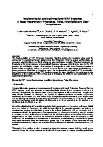
Figure 2: A simple relational data model

data sources in [15], formatted data files [6] and RDF [24]. For our purposes in the present paper, we assume that all schemas are specified in the very simple relational data model that we define below. However, we stress that the techniques that we describe here are equally applicable to any data modelling language supported by AutoMed. Schemas in our simple relational model are constructed from primary key attributes, non-primary key attributes, and the relationships between them. Figure 2 illustrates the representation of a relation R with primary key attributes k1 , ..., kn and non-primary key attributes a1 , ..., am . There is a one-one correspondence between this representation and the underlying HDM graph. In our simple relational model, there are two kinds of schema construct: Rel and Att (for simplicity, we ignore here the constraints present in a relational schema but see [13] for an encoding of a richer relational data model). The extent of a Rel construct hhRii is the projection of the relation R onto its primary key attributes k1 , ..., kn . The extent of each Att construct hhR, aii where a is an attribute (key or non-key) is the projection of relation R onto k1 , ..., kn , a. For example, a relation student(id,sex,dname) would be modelled by a Rel construct hhstudentii, and three Att constructs hhstudent, idii, hhstudent, sexii and hhstudent, dnameii1 . Once the constructs of modelling language M have been defined in terms of the HDM (via the API of AutoMed’s metadata repository [1]), a set of primitive schema transformations for M are automatically available. For the simple relational model above, these would be as follows: • addRel(hhRii, q) adds to the schema a new relation R. The query q specifies the set of primary key values in the extent of R in terms of the already existing schema constructs. • addAtt(hhR, aii, q) adds to the schema an attribute a (key or non-key) for relation R. The query q specifies the extent of the binary relationship between the primary key attribute(s) of R and this new attribute a in terms of the already existing schema constructs. • deleteRel(hhRii, q) deletes from the schema the relation R (provided all its attributes have first been deleted). The query q specifies how the extent of R can be restored from the remaining schema constructs. 1 We note that there is some redundancy of representation here, since the extent of each primary key attribute ki appears both within the extent of hhRii and within the extent of hhR, ki ii. We have adopted this representation for two main reasons. Firstly, it allows for easier integration of relational schemas with objectoriented schemas, in that hhRii corresponds to an OO class and each hhR, aii to an OO attribute. Secondly, this uniformity of treatment for all attributes allows for easier translation of IQL queries into SQL queries on local relational data sources.

5 LS1

staff(id,name,dname) male(id) female(id)

LS2

university(uname) campus(cmname,uname) dept(deptname,cmname) degree(dcode,title,dtype,deptname)

LS3

student(id,name,sex) enrolled(id,from,to,dcode) degree(dcode)

LS4

university(uname) college(cname,uname) dept(dname,street,cname)

USi

university(uname) campus(cmname,uname) dept(dname,street,cmname) degree(dcode,title,dtype,dname) staff(id,name,sex,dname) student(id,name,sex) enrolled(id,from,to,dcode)

GS

university(uname) campus(cmname,uname) dept(dname,street,cmname) degree(dcode,title,dtype,dname) person(id,name,sex,dname#) enrolled(id,from,to,dcode)

Figure 3: Example schemas

• deleteAtt(hhR, aii, q) deletes from the schema attribute a of relation R. The query q specifies how the extent of the binary relationship between the primary key attribute(s) of R and a can be restored from the remaining schema constructs. • renameRel(hhRii, hhR0 ii) renames the relation R to R0 in the schema. • renameAtt(hhR, aii, hhR, a0 ii) renames the attribute a of R to a0 . There is also a set of extendRel, extendAtt, contractRel and contractAtt primitive transformations.

2.1

An Example Integration

Figure 3 gives some specific schemas to illustrate the integration approach of Figure 1. Primary key attributes are underlined, foreign key attributes are in italics and nullable attributes are suffixed by #. In Example 1, transformations t1 –t5 use a composite transformation extendTable to state that the tables student, enrolled, university, campus and degree in US1 cannot be derived from LS1 . The definition of extendTable is: extendTable(hhR, a1 , . . . , an ii) = extendRel(hhRii, Void, Any) extendAtt(hhR, a1 ii, Void, Any) .. . extendAtt(hhR, an ii, Void, Any) Then transformations t6 –t9 use the dname attribute of staff to derive the dept table in US1 , and use extend transformations for the two attributes street and uname that cannot be derived from LS1 . Finally, in t10 –t14 the male and female relations of LS1 are restructured into the single sex attribute of staff.

6 The queries accompanying the add and delete transformations are expressed in our IQL intermediate query language. In IQL, ++ is the bag union operator and the construct [e | Q1 ; . . . Qn ] is a comprehension [2]. The expressions Q1 to Qn are termed qualifiers, each qualifier being either a filter or a generator. A filter is a boolean-valued expression. A generator has syntax p ← c where p is a pattern and c is a bag-valued expression. In IQL, the patterns p are restricted to be single variables or tuples of variables. Example 1 Pathway LS1 → US1 t1 extendTable(hhstudent, id, name, sexii) t2 extendTable(hhuniversity, unameii) t3 extendTable(hhcampus, cmname, unameii) t4 extendTable(hhdegree, dcode, title, dtype, dnameii) t5 extendTable(hhenrolled, id, from, to, dcodeii) t6 addRel(hhdeptii, [x | (y, x) ← hhstaff, dnameii]) t7 addAtt(hhdept, dnameii, [(x, x) | x ← hhdeptii]) t8 extendAtt(hhdept, streetii, Void, Any) t9 extendAtt(hhdept, unameii, Void, Any) t10 addAtt(hhstaff, sexii, [(x, ‘M’) | x ← hhmaleii] ++ [(x, ‘F’) | x ← hhfemaleii]) t11 deleteAtt(hhmale, idii, [(x, x) | x ← hhmaleii]) t12 deleteRel(hhmaleii, [x | (x, ‘M’) ← hhstaff, sexii]) t13 deleteAtt(hhfemale, idii, [(x, x) | x ← hhfemaleii]) t14 deleteRel(hhfemaleii, [x | (x, ‘F’) ← hhstaff, sexii]) The pathway LS2 → US2 contains extend steps to add the missing staff, student, and enrolled tables. It then renames deptname, and adds the missing attributes of dept: Example 2 Pathway LS2 → US2 t15 extendTable(hhstudent, id, name, sexii) t16 extendTable(hhstaff, id, name, sex, dnameii) t17 extendTable(hhenrolled, id, from, to, dcodeii) t18 renameAtt(hhdept, deptnameii, hhdept, dnameii) t19 renameAtt(hhdegree, deptnameii, hhdegree, dnameii) t20 extendAtt(hhdept, streetii, Void, Any) t21 extendAtt(hhdept, unameii, Void, Any) The pathway LS3 → US3 contains a sequence of extend steps for its missing information. The pathway LS4 → US4 creates in t22 a new attribute hhdept, unameii by joining the dept and college relations, and then deletes in t23 –t25 the college table that can be recovered from the remaining hhdept, cnameii attribute. Transformation t26 is unable to put any restriction on the values of hhdept, cnameii, since that association cannot be recovered from the global schema. Transformations t27 –t31 then perform the logical inverse of t22 –t26 to partially extract the campus table from the direct association between departments and universities represented by hhdept, unameii.

7 Example 3 Pathway LS4 → US4 t22 addAtt(hhdept, unameii, [(x, y) | (x, z) ← hhdept, cnameii; (z, y) ← hhcollege, unameii]) t23 deleteAtt(hhcollege, unameii, [(x, y) | (z, x) ← hhdept, cnameii; (z, y) ← hhdept, unameii]) t24 deleteAtt(hhcollege, cnameii, [(x, x) | x ← hhcollegeii]) t25 deleteRel(hhcollegeii, [y | (x, y) ← hhdept, cnameii]) t26 contractAtt(hhdept, cnameii, Void, Any) t27 extendAtt(hhdept, cmnameii, Void, Any) t28 addRel(hhcampusii, [y | (x, y) ← hhdept, cmnameii]) t29 addAtt(hhcampus, cmnameii, [(x, x) | x ← hhcampusii]) t30 addAtt(hhcampus, unameii, [(x, y) | (z, x) ← hhdept, cmnameii; (z, y) ← hhdept, unameii]) t31 delAtt(hhdept, unameii, [(x, y) | (x, z) ← hhdept, cmnameii; (z, y) ← hhcampus, unameii]) t32 extendTable(hhstudent, id, name, sexii) t33 extendTable(hhstaff, id, name, sex, dnameii) t34 extendTable(hhenrolled, id, from, to, dcodeii) Finally, we list in Example 4 the pathway from the union schema US1 to the global schema GS. The pathway from US2 , US3 or US4 would be identical. Example 4 Pathway US1 → GS t35 addRel(hhpersonii, hhstaffii ++ [x | x ← hhstudentii; not (member x hhstaffii)]) t36 addAtt(hhperson, idii, hhstaff, idii ++ [(x, y) | (x, y) ← hhstudent, idii; not (member x hhstaffii)]) t37 addAtt(hhperson, nameii, hhstaff, nameii ++ [(x, y) | (x, y) ← hhstudent, nameii; not (member x hhstaffii)]) t38 addAtt(hhperson, sexii, hhstaff, sexii ++ [(x, y) | (x, y) ← hhstudent, sexii; not (member x hhstaffii)]) t39 addAtt(hhperson, dnameii, hhstaff, dnameii) t40 contractAtt(hhstudent, idii, [(x, y) | (x, y) ← hhperson, idii; not (member x hhstaffii)], [(x, y) | (x, y) ← hhperson, idii]) t41 contractAtt(hhstudent, nameii, [(x, y) | (x, y) ← hhperson, nameii; not (member x hhstaffii)], [(x, y) | (x, y) ← hhperson, nameii]) t42 contractAtt(hhstudent, sexii, [(x, y) | (x, y) ← hhperson, sexii; not (member x hhstaffii)], [(x, y) | (x, y) ← hhperson, sexii]) t43 contractRel(hhstudentii), [x | x ← hhpersonii; not (member x hhstaffii)], [x | x ← hhpersonii]) t44 deleteAtt(hhstaff, idii, [(x, y) | (x, y) ← hhperson, idii; member x hhstaffii]) t45 deleteAtt(hhstaff, nameii, [(x, y) | (x, y) ← hhperson, nameii; member x hhstaffii]) t46 deleteAtt(hhstaff, sexii, [(x, y) | (x, y) ← hhperson, sexii; member x hhstaffii]) t47 deleteAtt(hhstaff, dnameii, hhperson, dnameii) t48 deleteRel(hhstaffii, [x | (x, y) ← hhperson, dnameii]) We assume in this example integration that a person may be both a member of staff and a student. For such people, their information in the staff table is preferred for propagation to the global person table in steps t35 –t38 above. Thus, there is not sufficient information in the global schema to totally derive the student table, and only contract statements can be given in steps t40 –t43 , where as a lower bound we know all persons not in the staff table are students, but as an upper bound know that all persons could be in student (if it were the case that all staff members were former students). Conversely, there is sufficient information to totally derive the staff table.

8

2.2

Comparison of BAV with GAV, LAV and GLAV

We see from the above example that the add and extend steps in the transformation pathways from the local schemas to the global schema correspond to GAV, since it is these steps that are incrementally defining global constructs in terms of local ones. Similarly, it is the delete and contract steps in the transformation pathways from the local schemas to the global schema that correspond to LAV, since it is these steps that are incrementally defining local constructs in terms of global ones. We will see in Section 3 how these pathways can be traversed to derive GAV and LAV views. If a GAV view is derived from solely add steps it will be exact in the terminology of [7]. If, in addition, it is derived from one or more extend steps using their lower-bound (upper-bound) queries, then the GAV view will be sound (complete) in the terminology of [7]. Similarly, if a LAV view is derived solely from delete steps it will be exact. If, in addition, it is derived from one or more contract steps using their lower-bound (upper-bound) queries, then the LAV view will be complete (sound) in the terminology of [7]. For example, in pathway US1 → GS above, we could enhance t43 above to: contractRel(hhstudentii, [x | x ← hhpersonii; not (member x hhstaffii)], hhpersonii]) asserting that hhstudentii contains the set of people who are not staff (completeness) and is contained by the whole set of people (soundness). As we discussed in the introduction, BAV is a more expressive data integration language than LAV, GAV or GLAV, since it allows for the expression of mappings in both directions, and since it is not limited on how many source schemas are associated by a mapping. Indeed, in the context of peer-to-peer integration, [3] has suggested using GLAV rules in both directions in a similar manner to BAV, in order to overcome weaknesses of using GLAV alone. As discussed in [16, 17], a further advantage of BAV over GAV and LAV is that it readily supports the evolution of both global and local schemas, by allowing pathways and schemas to be incrementally modified as opposed to having to be regenerated. A further difference between BAV and GAV, LAV or GLAV (including the approach of using GLAV in each direction of [3]) is that statements about the relationships between global and local schemas are made at a finer level of detail, i.e. at the level of individual attributes as opposed to entire tables. So we can assert exact knowledge about some attributes of a table, and sound or complete knowledge about other attributes. We are also able to introduce intermediate constructs in the mapping, such as in LS4 → US4 .

3

Generating Views

We now present a general technique for generating GAV, LAV and GLAV view definitions from a BAV pathway. This ability to generate any of these kinds of view definitions from a single BAV pathway means that we can select a query processing technique that can vary between queries as appropriate. To define a construct c in Sx in terms of the constructs in schema Sy , we consider in turn the transformations of Sx → Sy . The only transformations that are significant are those that delete, contract or rename a construct2 . These transformations are significant because the current view definitions may query constructs that no longer exist after such a transformation. Each of these types of transformation is handled as follows if it is encountered during the 2

Note that this is equivalent to considering the add, extend and rename steps in the reverse S y → Sx

9 traversal of Sx → Sy : • delete: This has an associated query which shows how to reconstruct the extent of the construct being deleted. Any occurrence of the deleted construct within the current view definitions is replaced by this query. • contract: Any occurrence of the contracted construct within the current view definitions is replaced by either the lower-bound or the upper-bound query accompanying this transformation step, depending on whether sound or complete views are required. • rename: All references to the old construct in the current view definitions are replaced by references to the new construct.

3.1

Generating GAV Views

To generate the set of GAV views for a global schema, the pathways from it to each local schema are retrieved from AutoMed’s metadata repository. For some part of the start of their length these pathways may be the same, as may be seen from the tree structure of Figure 1. Each node of this transformations tree is a schema (global, intermediate or local) linked to its neighbours by a single transformation step. View definitions for each global schema construct are derived by traversing the tree from top to bottom. Initially, each construct’s view definition is just the construct itself. Each node in the tree is then visited in a downwards direction, and delete, contract and rename transformations are handled as described above. In particular, if a contract transformation step is encountered, any occurrence of the contracted construct within the current GAV view definitions is replaced by the lower-bound query accompanying this transformation step (so that sound GAV views will be generated). At some points the tree may branch. When this happens, constructs of the parent schema are semantically identical to constructs that have the same scheme within the child schemas. The possibility of using all paths is retained within the view definitions by replacing each construct of the parent schema by a disjunction (OR) of the corresponding constructs in the child schemas. The tree is traversed in this fashion from the root to the leaves until all the nodes are visited. The resulting view definitions are the GAV definitions for the global schema constructs over the local schemas. Referring again to the example of Section 2.1, consider the construct GS : hhperson, sexii in the global schema. The pathway GS → US1 would be processed first (i.e. the reverse of the pathway US1 → GS listed in Section 2.1). The only significant transformation is t38 that deletes hhperson, sexii, resulting in an intermediate view definition: GS : hhperson, sexii :US1 : hhstaff, sexii ++ [(x, y) | (x, y) ← US1 : hhstudent, sexii; not (member x US1 : hhstaffii)] at one copy, US1 , of the four union schemas. Traversing the pathways US1 → LS1 and US1 → US2 , we replace the body of the view definition with: ( [(x, ‘M’) | x ← LS1 : hhmaleii] ++ [(x, ‘F’) | x ← LS1 : hhfemaleii] OR US2 : hhstaff, sexii) ++ ( [(x, y) | (x, y) ← Void OR US2 : hhstudent, sexii; not (member x (LS1 : hhstaffii OR US2 : hhstaffii))]) Traversing next US2 → LS2 and US2 → US3 , we get: ( [(x, ‘M’) | x ← LS1 : hhmaleii] ++ [(x, ‘F’) | x ← LS1 : hhfemaleii]) OR Void OR US3 : hhstaff, sexii) ++ ( [(x, y) | (x, y) ← Void OR Void OR US3 : hhstudent, sexii; not (member x (LS1 : hhstaffii OR Void OR US3 : hhstaffii))])

10 Continuing with US3 → LS3 and US3 → US4 , we get: ( [(x, ‘M’) | x ← LS1 : hhmaleii] ++ [(x, ‘F’) | x ← LS1 : hhfemaleii]) OR Void OR Void OR US4 : hhstaff, sexii) ++ ( [(x, y) | (x, y) ← Void OR Void OR LS3 : hhstudent, sexii OR US4 : hhstudent, sexii; not (member x (LS1 : hhstaffii OR Void OR Void OR US4 : hhstaffii))]) Traversing finally US4 → LS4 , we obtain the view definition: GS : hhperson, sexii :( [(x, ‘M’) | x ← LS1 : hhmaleii] ++ [(x, ‘F’) | x ← LS1 : hhfemaleii]) OR Void OR Void OR Void) ++ ( [(x, y) | (x, y) ← Void OR Void OR LS3 : hhstudent, sexii OR Void; not (member x (LS1 : hhstaffii OR Void OR Void OR Void))]) Section 4 will justify how this view definition can be simplified to: GS : hhperson, sexii :( [(x, ‘M’) | x ← LS1 : hhmaleii] ++ [(x, ‘F’) | x ← LS1 : hhfemaleii])) ++ ( [(x, y) | (x, y) ← LS3 : hhstudent, sexii; not (member x (LS1 : hhstaffii))]) Such view derivations can be substituted into any query posed on a global schema in order to obtain an equivalent query distributed over the local schemas — this is the GAV approach to global query processing, which is what the AutoMed implementation currently supports.

3.2

Generating LAV Views

LAV views are derived similarly: the pathway from a local schema to the global schema is again retrieved from the metadata repository and is processed as above to derive the view definitions, except that it is the local schema end of the pathway that is now taken as the root of the tree. The derivation of LAV views is simpler because there is now only a single pathway being processed, with no branching. Also, if a contract transformation step is encountered, any occurrence of the contracted construct within the current LAV view definitions is replaced by the upper-bound query accompanying this transformation step (so that sound LAV views will be generated). For example, to generate a LAV definition of LS1 : hhmaleii, we inspect the pathway t1 ,..,t14 ,t35 ,..,t48 . The transformation t12 deletes hhmaleii, and therefore we have an intermediate view definition on US1 : LS1 : hhmaleii :- [x | (x, ‘M’) ← US1 : hhstaff, sexii] Then hhstaff, sexii construct is deleted by t46 , which substitutes(x, y) ← hhstaff, sexii with (x, y) ← hhperson, sexii; member x hhstaffii, and the hhstaffii construct in this query is deleted by t40 giving a final LAV rule: LS1 : hhmaleii :- [x | (x, ‘M’) ← GS : hhperson, sexii; member x [x | (x, y) ← GS : hhperson, dnameii]]

3.3

Generating GLAV Views

First, it should be noted that GLAV view definitions will include all the LAV view definitions, and all the GAV view definitions where the body of the rule is a query that matches the conditions required for the GLAV query processing system in use (which in [11] would be queries over a single source). In addition, we inspect now all the add and extend transformations of the pathway that would be ignored by LAV view generation, and for each one use the query to form the head of a new GLAV rule. For example, in LS4 → US4 , the query in t22 gives a new view rule head:

11 [(x, y) | (x, z) ← LS4 : hhdept, cnameii; (z, y) ← LS4 : hhcollege, unameii] which is defined by hhdept, unameii at this stage. We then use our standard algorithm on construct hhdept, unameii, detect that it is deleted in t31 , and hence replace it with the query from t31 to result in the GLAV rule: [(x, y) | (x, z) ← LS4 : hhdept, cnameii; (z, y) ← LS4 : hhcollege, unameii] :[(x, z) | GS : hhdept, cmnameii; (z, y) ← GS : hhcampus, unameii] Note however that the BAV integration would still hold if LS4 were fragmented, with campus and departments held on separate sources, whereas GLAV would cease to be valid in this situation.

4

Optimising the Generated Views

The view definitions generated by the process described above can be simplified after they have been derived. This saves later work for the query optimiser when these definitions are substituted into specific global queries for query processing. It also means that our generated views end up looking much like views that would have been specified directly in a GAV, LAV or GLAV framework. The AutoMed intermediate query language IQL supports two kinds of operator for manipulating bags: the bag append operator, ++, and also a family of operators which are all semantically based on a single function, fold. fold applies a given function f to each element of a bag and then ‘folds’ a binary operator op into the resulting values. It is defined as follows, where [] is the empty bag, [x] is a singleton bag containing one element x, and b1 ++ b2 is the union of two bags b1 and b2: fold f op e [] = e fold f op e [x] = f x fold f op e (b1 ++ b2) = (fold f op e b1) op (fold f op e b2) For example, sum = fold (id) (+) 0 and count = fold (lambda x.1) (+) 0. The other common grouping and aggregation operators can also be defined in terms of fold, as can a function flatmap: flatmap f b = fold f (++) [] b flatmap can in turn be used to define selection, projection, and join operators. The comprehension syntax mentioned earlier also translates into successive applications of flatmap. Optimisations for fold apply to all operators that can be defined in terms of it, including selection, projection, join, group-by, aggregation, and comprehensions. Regarding the view definitions generated from BAV pathways as described in the previous section, there are two particular optimisations that can be applied to them. Firstly, instances of Void can be removed. For the purposes of query processing, Void is regarded as being equal to the empty bag. Thus: fold f op e Void flatmap f Void group Void gc f Void sum Void

= = = = =

fold f op e [] flatmap f [] group [] gc f [] sum []

= = = = =

e [] [] [] 0

12 count Void Void ++ e Void OR e

= count [] = 0 = [] ++ e = e ++ [] = e ++ Void = e = e OR Void = e

where group groups a bag of pairs according to common values in their first component and gc f groups a bag of pairs according to common values in their first component and then applies an aggregation function f to the resulting groups of second components. We refer the reader to [19] for more details of IQL and for references to work on fold-based functional query languages and optimisation techniques for such languages. Due to the step-wise specification of our schema transformations, there is a second major optimisation which may be applicable. This is known as loop fusion and it replaces two successive iterations over a collection by one iteration provided the operators in question satisfy certain algebraic properties. A simple instance of loop fusion is the standard relational query optimisation πA (πB (R)) = πA,B (R). Loop fusion does not arise in the schema integration example of Section 2.1 but consider the following fragment of an AutoMed pathway. This first joins two schemes hhR, aii and hhR, bii, creating an intermediate relation hhIii, and then projects onto the a and b attributes, creating a relation hhV ii, and finally deletes hhIii: addRel(hhIii, [(x, y, z) | (x, y) ← hhR, aii; (x, z) ← hhR, bii]) addRel(hhV ii, [(y, z) | (x, y, z) ← hhIii]) deleteRel(hhIii, [(x, y, z) | (x, y) ← hhR, aii; (x, z) ← hhR, bii]) The view definition generated for hhV ii would be [(y, z) | (x, y, z) ← [(x, y, z) | (x, y) ← hhR, aii; (x, z) ← hhR, bii]]) and the generator (x, y, z) ← in the outer comprehension can be fused with the head expression of the inner comprehension, giving: [(y, z) | (x, y) ← hhR, aii; (x, z) ← hhR, bii] There are a range of other standard algebraic optimisations that could be performed on the view definitions e.g. pushing down selections and projections. However, these kinds of optimisations will also be applied later, when a specific global query is reformulated by substituting into it the view definitions. Further optimisations and rewrites will be applied at this stage e.g. to bring constructs from the same local schemas together into sub-queries which can be posed entirely on one local schema and it is these sub-queries (appropriately translated) that will be sent to local data sources for evaluation.

5

Validating and Optimising Pathways

One important feature of the AutoMed approach is that once a set of schemas have been joined in a network of pathways, data and queries may be translated or migrated between any pair of schemas in the network. Such networks may be complex to analyse, so we need to support automated validation that a network is well-formed. We also need to support automated optimisation of the pathways between schemas, since they may contain redundant transformations. To support such validation and optimisation of pathways, we have developed the Transformation Manipulation Language (TML) [23], which represents each transformation in a form suited to analysis of the schema constructs that are created, deleted or are required to be present for the transformation to be correct. Our definitions below require a function sc that given a query determines all schema constructs that must exist if the query is valid. For the IQL language constructs used in our earlier examples, sc is defined as:

13 sc(hhrii) = hhrii sc(hhr, aii) = {hhrii, hhr, aii} sc([q1 , . . . , qn ]) = sc(q1 ) ∪ . . . ∪ sc(qn ) sc(q1 ++ q2 ) = sc(q1 ) ∪ sc(q2 ) sc([q | q1 , . . . , qn ]) = sc(q) ∪ sc(q1 ) ∪ . . . ∪ sc(qn ) Note that as a shorthand, we will write the pair of queries ql , qu in extend or contract as just q, with the semantics in such cases that sc(ql , qu ) = sc(ql ) ∪ sc(qu ). The TML formalises each − + − transformation ti of schema Si into schema Si+1 as having four conditions a+ i , bi , c i , d i : • The positive precondition a+ i is the set of constructs that ti implies must be present in Si . It comprises those constructs that are present in the query of the transformation (given by sc(q)) together with any constructs implied as being present by the construct c: ti ∈ {add(c, q), extend(c, q)} → a+ i = (sc(c) − c) ∪ sc(q) ti ∈ {delete(c, q), contract(c, q), rename(c, c0 ), id(c, c0 )} → a+ i = sc(c) ∪ sc(q)

• The negative precondition b− i is the set of constructs that ti implies must not be present in Si . It comprises those constructs which the transformation will add to the schema, and thus must not already be present: ti ∈ {add(c, q), extend(c, q), rename(c0 , c), id(c0 , c)} → b− i =c ti ∈ {delete(c, q), contract(c, q)} → b− i =∅

• The positive postcondition c+ i is the set of constructs that ti implies must be present in Si+1 , and is derived in the same way as a+ i (i.e. the positive precondition of the ti ): ti ∈ {add(c, q), extend(c, q), rename(c0 , c), id(c0 , c)} → c+ i = sc(c) ∪ sc(q) ti ∈ {delete(c, q), contract(c, q)} → c+ i = (sc(c) − c) ∪ sc(q)

• The negative postcondition d− i is the set of constructs that ti implies must not be present in Si+1 , and is derived in the same way as b− i : ti ∈ {delete(c, q), contract(c, q), rename(c, c0 ), id(c, c0 )} → d− i = c, ti ∈ {add(c, q), extend(c, q)} → d− i =∅

We can express LS1 → US1 in TML as shown below. Note that compound transformations such as t1 are first expanded into their primitive transformations before being converted into the TML. t1.1 t1.2 t1.3 t1.4

: [∅, {hhstudentii}, {hhstudentii}, ∅] : [∅, {hhstudent, idii}, {hhstudentii, hhstudent, idii}, ∅] : [∅, {hhstudent, idii}, {hhstudentii, hhstudent, sexii}, ∅] : [∅, {hhstudent, idii}, {hhstudentii, hhstudent, dnameii}, ∅]

.. . t6 t7 t8 t9

: [{hhstaffii, hhstaff, dnameii}, {hhdeptii}, {hhdeptii, hhstaffii, hhstaff, dnameii}, ∅] : [{hhdeptii}, {hhdept, dnameii}, {hhdeptii, hhdept, dnameii}, ∅] : [{hhdeptii}, {hhdept, streetii}, {hhdeptii, hhdept, streetii}, ∅] : [{hhdeptii}, {hhdept, unameii}, {hhdeptii, hhdept, unameii}, ∅]

14 t10 t11 t12 t13 t14

5.1

: [{hhstaffii, hhmaleii, hhfemaleii}, {hhstaff, sexii}, {hhstaffii, hhstaff, sexii, hhmaleii, hhfemaleii}, ∅] : [{hhmaleii, hhmale, idii}, ∅, {hhmaleii}, {hhmale, idii}] : [{hhmaleii, hhstaffii, hhstaff, sexii}, ∅, {hhstaffii, hhstaff, sexii}, {hhmaleii}] : [{hhfemaleii, hhfemale, idii}, ∅, {hhfemaleii}, {hhfemale, idii}] : [{hhfemaleii, hhstaffii, hhstaff, sexii}, ∅, {hhstaffii, hhstaff, sexii}, {hhfemaleii}]

Well-formed Transformation Pathways

A pathway T from schema Sm to Sn is said to be well-formed if for each transformation step ti : Si → Si+1 within it: • The only difference between the schema constructs in Si+1 and Si is those constructs − specifically changed by transformation ti , implying that Si+1 = (Si ∪ c+ i ) − di and − + Si = (Si+1 ∪ ai ) − bi − • The constructs required by ti are in the schemas, implying that a+ i ⊆ Si , bi ∩ Si = ∅, − + ci ⊆ Si+1 and di ∩ Si+1 = ∅

The above definition leads to the recursive definition of a well-formed pathway, wf , given below. The first rule applies each transformation step in turn, and the second rule ensures that the schema that results from applying all the transformation steps is equal to the schema at the end of the pathway (equal both in terms of the schema constructs found in each schema and the extent of the schemas). Note that any implementation may use these rules in two ways. Firstly, given a schema Sm representing a data source, and pathway P , a new data source schema Sn and its extent can be derived. Secondly, if Sn exists as a data source already, a check can be made to verify that P correctly derives its schema and extent from that of Sm . − wf (Sm , Sn , [tm , tm+1 , . . . , tn−1 ]) ← a+ m ⊆ S m ∧ bm ∩ S m = ∅ ∧ − wf ((Sm ∪ c+ m ) − dm , Sn , [tm+1 , . . . , tn−1 ])

wf (Sm , Sn , []) ← Sm = Sn ∧ Ext(Sm ) = Ext(Sn )

5.2

Reordering of Transformations

Certain transformations may be performed in any order, whilst others must be performed in a specific order. For example, in LS1 → US1 , t11 must be performed before t12 , since the attribute hhmale, idii must be deleted before the hhmaleii relation is deleted. However the subpathway t11 ,t12 could be performed before or after the sub-pathway t13 ,t14 since it does not matter which of the hhmaleii or hhfemaleii relations is deleted first. In the TML, this intuition is expressed by stating that transformations may be swapped provided the pathway remains well-formed. This may be verified by inspecting the conditions of each transformation. In particular, a pair of transformations t i ,ti+1 may be reordered to ti+1 ,ti provided: 1. ti does not add a construct that is required by ti+1 , and ti+1 does not add a construct + + + + + that is required by ti , i.e. (c+ n − an ) ∩ ai+1 = ∅ and (ai+1 − ci+1 ) ∩ cn = ∅

15 2. ti does not delete a construct required not to be present by ti+1 , and ti+1 does not delete + a construct required not to be present by ti , i.e. d+ n ∩ bi+1 = ∅ We can now formalise the two examples given above from LS1 → US1 . For t11 ,t12 , (1) is broken, and hence they may not be swapped. The changing of t11 ,t12 ,t13 ,t14 to t13 ,t14 ,t11 ,t12 may be performed by iteratively swapping pairs of transformations. Considering first t 12 ,t13 , we find neither rule is broken, and they may be reordered to t13 ,t12 . Then t12 ,t14 breaks neither rule, and may be reordered to t14 ,t12 . This leaves a sub-pathway t11 ,t13 ,t14 ,t12 , and a similar argument allows t11 swap with t13 and then t14 , to give the sub-pathway t13 ,t14 ,t11 ,t12 .

5.3

Redundant Transformations

Two transformations tx and ty in a well-formed pathway T are redundant if T may be reordered such that tx and ty become consecutive within it, and T remains well-formed if they are then removed. Such redundant transformations will occur if a source schema evolves to model information in the same way as the global schema when previously it modelled the information in a different way. For example, suppose LS1 is evolved by transformations t49 ,t50 ,t51 ,t52 ,t53 , textually identical to transformations t10 ,t11 ,t12 ,t13 ,t14 , to model the gender of staff as a single sex attribute in a new version of the schema LS01 . By reversing these transformation steps we can derive the pathway from the new to the old schema LS 01 → LS1 : Example 5 Pathway LS01 → LS1 t53 addRel(hhfemaleii, [x | (x, ‘F’) ← hhstaff, sexii]) t52 addAtt(hhfemale, idii, [(x, x) | x ← hhfemaleii]) t51 addRel(hhmaleii, [x | (x, ‘M’) ← hhstaff, sexii]) t50 addAtt(hhmale, idii, [(x, x) | x ← hhmaleii]) t49 deleteAtt(hhstaff, sexii, [(x, ‘M’) | x ← hhmaleii] ++ [(x, ‘F’) | x ← hhfemaleii]) If we inspect the entire path LS01 → US1 , consisting of LS01 → LS1 followed by LS1 → US1 , it may be reordered to contain the sub-pathway: t51 addRel(hhmaleii, [x | (x, ‘M’) ← hhstaff, sexii]) t50 addAtt(hhmale, idii, [(x, x) | x ← hhmaleii]) t49 deleteAtt(hhstaff, sexii, [(x, ‘M’) | x ← hhmaleii] ++ [(x, ‘F’) | x ← hhfemaleii]) t10 addAtt(hhstaff, sexii, [(x, ‘M’) | x ← hhmaleii] ++ [(x, ‘F’) | x ← hhfemaleii]) t11 deleteAtt(hhmale, idii, [(x, x) | x ← hhmaleii]) t12 deleteRel(hhmaleii, [x | (x, ‘M’) ← hhstaff, sexii]) Clearly t49 ,t10 forms a redundant pair, because we are adding and deleting the same construct with the same extent since the query is the same. Once this has been performed t50 ,t11 may be removed for the same reason, and then t51 ,t12 . Once all other redundant pairs have been removed, LS01 → US1 would comprise of just t1 –t9 . Using the TML, we can identify redundant transformations as satisfying: + − − + + − − + + + + (a+ x = cy ) ∧ (bx = dy ) ∧ (cx = ay ) ∧ (dx = by ) ∧ Ext(cx ⊕ ax ) = Ext(cy ⊕ ay ) where (x ⊕ y) = (x − y) ∪ (y − x), and thus serves to find all the constructs being added or deleted by the pair of transformations. In practice, this rule means that any pair of transformations which add/extend and then delete/contract (in either order) the same construct are redundant, providing the query can be demonstrated to result in the same extent.

16

5.4

Partially Redundant Transformations

Two transformations tx and ty in a well-formed pathway T are partially redundant if T may be reordered to make tx and ty consecutive, and T remains well-formed if they are then replaced by a single transformation txy . The pathway LS1 → LS2 has a pair of such partially redundant transformations, since it can be reordered to obtain the sub-pathway: t7 addAtt(hhdept, dnameii, [(x, x) | x ← hhdeptii]) t18 renameAtt(hhdept, dnameii, hhdept, deptnameii) This may be replaced by the new transformation given below, which leaves a fully optimised pathway LS1 → LS2 . t54 addAtt(hhdept, deptnameii, [(x, x) | x ← hhdeptii]) Using the TML, we can identify partially redundant transformations as satisfying: + − − − − − − (a+ x = cy ⊕ bx = dy ) ∧ dx ∩ by = ∅ ∧ dx 6= ∅ ∧ by 6= ∅ The simplifications for removing partially redundant and fully redundant transformations are summarised in the table below. The table shows what simplifications may be applied where a pair of transformations is found to operate on the same construct c. NWF denotes ‘not well-founded’ and [ ] denotes the removal of the pair. The table would remain correct if extend were to replace add, contract replace delete, and id replace rename. Further details of redundant and partially redundant transformations may be found in [23].

add(c,q) add(c,q) NWF tx delete(c,q) [ ] rename(c’,c) NWF rename(c”,c) NWF

6

ty delete(c,q) [] NWF delete(c’,q) delete(c”,q)

rename(c,c’) add(c’,q) NWF [] rename(c”,c’)

Concluding Remarks

In this paper we have described view generation and view optimisation in the AutoMed heterogeneous database integration framework. We have shown how the AutoMed schema pathways and views generated from them are amenable to considerable simplification, resulting in view definitions that look much like the views that would have been specified directly in a GAV, LAV or GLAV framework. Since BAV integration is based on sequences of primitive schema transformations, it could be argued that data integration using it is more complex than with GAV, LAV or GLAV. However, the integration process can be greatly simplified by specifying well-known schema equivalences as higher-level composite transformations. We gave such an example, extendTable, in Section 2.1 above, and further examples are given in [17]. Moreover, we are working on techniques for semi-automatically generating transformation pathways to convert a source schema expressed in one modelling language into an equivalent target schema expressed in another modelling language, based on well known schema equivalences. We are also investigating schema matching techniques to automatically or semi-automatically integrate two specific schemas. Finally, it should be noted that BAV is well-suited to peer-to-peer data integration (see [18]) since it lacks the directionality inherent in LAV, GAV and GLAV, all of which are tied to

17 the concept of there being a global schema which may not always be the case in peer-to-peer environments.

References [1] M. Boyd, P.J. McBrien, and N. Tong. The automed schema integration repository. In Proc. BNCOD02, LNCS 2405, pages 42–45, 2002. [2] P. Buneman et al. Comprehension syntax. ACM SIGMOD Record, 23(1):87–96, 1994. [3] D. Calvanese, E. Damagio, G. De Giacomo, M. Lenzerini, and R. Rosati. Semantic data integration in P2P systems. In Proceedings of DBISP2P, Berlin, Germany, 2003. [4] S.S. Chawathe et al. The TSIMMIS project: Integration of heterogeneous information sources. In Proc. 10th Meeting of the Information Processing Society of Japan, pages 7–18, October 1994. [5] M. Friedman, A. Levy, and T. Millstein. Navigational plans for data integration. In Proc.16th National Conf. on AI, pages 67–73. AAAI Press, 1999. [6] S. Kittivoravitkul. Transformation-based approach for integrating semi-structured data. Technical report, AutoMed Project, 2003. [7] M. Lenzerini. Data integration: A theorectical perspective. In Proc. PODS02, pages 247–258, 2002. [8] A.Y. Levy. Logic-based techniques in data integration. In J. Minker, editor, Logic Based Artificial Intelligence. Kluwer Academic Publishers, 2000. [9] A.Y. Levy, A.O. Mendelzon, Y. Sagiv, and D. Srivastava. Answering queries using views. In Proc. PODS’95, pages 95–104. ACM Press, May 1995. [10] A.Y. Levy, A. Rajamaran, and J.Ordille. Querying heterogeneous information sources using source description. In Proc. VLDB’96, pages 252–262, 1996. [11] J. Madhavan and A.Y. Halevy. Composing mappings among data sources. In Proceedings of 29th Conference on VLDB, pages 572–583, 2003. [12] I. Manolescu, D. Florescu, and D. Kossmann. Answering XML queries on heterogeneous data sources. In Proc. VLDB’01, pages 241–250, 2001. [13] P.J. McBrien and A. Poulovassilis. Automatic migration and wrapping of database applications — a schema transformation approach. In Proc. ER’99, LNCS 1728, pages 96–113, 1999. [14] P.J. McBrien and A. Poulovassilis. A uniform approach to inter-model transformations. In Proc. CAiSE’99, LNCS 1626, pages 333–348, 1999. [15] P.J. McBrien and A. Poulovassilis. A semantic approach to integrating XML and structured data sources. In Proc. CAiSE’01, LNCS 2068, pages 330–345, 2001.

18 [16] P.J. McBrien and A. Poulovassilis. Schema evolution in heterogeneous database architectures, a schema transformation approach. In Proc. CAiSE’02, LNCS 2348, pages 484–499, 2002. [17] P.J. McBrien and A. Poulovassilis. Data integration by bi-directional schema transformation rules. In Proc. ICDE’03, 2003. [18] P.J. McBrien and A. Poulovassilis. Defining peer-to-peer data integration using both as view rules. In Proceedings of DBISP2P, Berlin, Germany, 2003. [19] A. Poulovassilis. The AutoMed Intermediate Query Language. Technical report, AutoMed Project, 2001. [20] A. Poulovassilis and P.J. McBrien. A general formal framework for schema transformation. Data and Knowledge Engineering, 28(1):47–71, 1998. [21] M.T. Roth and P. Schwarz. Don’t scrap it, wrap it! A wrapper architecture for data sources. In Proc. VLDB’97, pages 266–275, Athens, Greece, 1997. [22] M. Templeton, H.Henley, E.Maros, and D.J. Van Buer. InterViso: Dealing with the complexity of federated database access. The VLDB Journal, 4(2):287–317, 1995. [23] N. Tong. Database schema transformation optimisation techniques for the AutoMed system. Technical report, AutoMed Project, 2002. [24] D. Williams. Representing RDF and RDF Schema in the HDM. Technical report, Automed Project, 2002.