EYE on EDUCATION
Virtual and Remote Control Labs Using Java: A Qualitative Approach By J. Sánchez, F. Morilla, S. Dormido, J. Aranda, and P. Ruipérez
I
n our modern society, distance education has become a viable solution for students who require more flexible, accessible, and adaptive teaching systems, without spatial and temporal restrictions [1], [2]. In the past, the interaction methods for distance education were limited to the telephone, postal mail, or fax. Today’s new information technologies provide alternative tools for improving teacher-student interaction, two of which can be pointed to as the most capable and reliable for distance education. These tools are hypermedia systems as a new way of arranging information and wide-area communication networks (i.e., the Internet) for information support [3]. Although these tools are sufficient for constructing support systems for subjects without a strong practical component, teaching of control systems or other subjects with strong experimental content requires a new element. This new element must allow students to apply the knowledge acquired in a way that goes beyond the traditional physical laboratory, which requires the presence of students as well as an instructor or tutor [4], [5]. If the laboratory environment is to be transferred to distance education, the element required to put automatic control concepts into practice is the virtual control laboratory [6]-[9]. An even more ambitious prospect is a virtual control laboratory with telepresence systems, which offers the stimulating possibility of students having remote control of the physical systems in place at the university lab [10]-[14]. Today, numerous commercial and university computer tools are available for the analytical study of control systems from a purely graphic or a numerical viewpoint, or a combination of both approaches [15]-[18]. These quantitative tools require the user to have a university-level knowledge of mathematics and a solid background in control systems. This article describes a new way of teaching adopted at the Universidad Nacional de Educación a Distancia (UNED) that uses dynamic and interactive simulations in a stand-alone or Web-based environment. The article focuses on how this new stand-alone experimentation environment maintains a clear separation between the graphical experimentation interface, developed in Java, and the math and simulation engine. By constructing the environment in this fashion, the math engine can be replaced with a different one or with a real plant, or can even be ported to a remote server. A Web-based, multiuser virtual lab is also possible without the necessity of reprogramming the experimenta-
tion interface code. Other differences with respect to tools are the dynamic simulations, the user interactivity, the generation of new experiments as goals change, and the opportunity to practice with classical or advanced control strategies in different plants: a heat exchanger, a tank, a distillation column, or an inverted pendulum. The article is organized as follows. First, we discuss our reasons for constructing such an environment. Next, we describe the various elements of the environment and the types of experiments that can be built to provide students with new practical experiences. Following that is a discussion of the tools used to construct the environment and the communication mechanisms between them. Finally, we describe options for replacing the math engine (MATLAB/ Simulink) and the porting of the stand-alone environment from a local to a Web-based environment. The Appendix gives a detailed description of how to link the Java experimentation interface and the MATLAB workspace.
Why Is a Conceptual Laboratory Needed? The idea of this virtual laboratory arises from the necessity for a suitable system that can be used by two different groups of people: plant operators and university students. Those in the first group typically have only a basic (high-school level) mathematics background, but they work on a daily basis with real control systems. They usually interact with the industrial environment through control panels, although at times they have contact with actual devices. University students, on the other hand, have a strong mathematics and control engineering background, but, except for experiments carried out at the university laboratory (e.g., inverted pendulum, dc motor, magnetic levitation), they have little experience with how industrial plants operate. Therefore, they are unable to anticipate how systems will react in certain situations. Thus, a qualitative teaching/training system is a useful tool for learning how to deal with certain cases. Using this method, two of the current problems in distance teaching are solved: temporary availability and the training aspect. Students/operators can practice anywhere at any time, without the need to go to a training center or keep to a timetable (the teaching/training system will be available 24 hours a day via their computers). At the same time, because the environment is interactive, the users can simulate plant operations that they would otherwise have to experience in actual situations.
Sánchez (
[email protected]), Morilla, Dormido, Aranda, and Ruipérez are with the Dpto. de Informática y Automática, UNED, Avda. Senda del Rey no. 9, 28040 Madrid, Spain. 8
0272-1708/02/$17.00©2002IEEE IEEE Control Systems Magazine
April 2002
Figure 1. Interface for basic control of a heat exchanger.
Figure 2. Interface for cascade control of a heat exchanger.
Figure 3. Interface for level control of a horizontal tank without a pump.
Figure 4. Interface for advanced control of a distillation column.
This work is not intended to develop a powerful universal control panel that is adaptable to any industrial system. For educational purposes, it is more appropriate to begin with an understanding of the basic components of an industrial plant and provide the student/operator an individualized environment with a collection of actual plant elements (i.e., heat exchangers, tanks, distillation columns). Typical university laboratory experiments such as inverted pendulums and magnetic levitators are also included. Although the environment encourages individual work, the trainer/tutor role is still important. Obviously, students/operators can interact with the environment, but without the appropriate instructional support, they will be unable to take full advantage of it. Thus, the tutor/instructor plays an essential role, with responsibility for adapting the configuration and behavior of the training environment according to educational needs. As will be seen later, this is possible because the entire system is parameter based at different levels.
This environment is also useful to help the teacher bring the theoretical concepts (which are basically quantitative) to the practical world (which is more qualitative and intuitive).
April 2002
Dynamic Experimentation Environment The simulation environment is completely interactive and dynamic (no batch or offline simulations). In this way, the qualitative aspects are immediately highlighted graphically and numerically as a response to the user’s actions. Students are not expected merely to tune sliders and controllers, to run the simulation, to examine the “scopes” (displays), and to repeat all the steps if they want to change some of the data. During the experimentation phase, changes in parameters and variables are immediately reflected in the graphical user interface (GUI). Thus, users can visualize on the fly how the model behavior evolves according to the values of the interactive variables. The simulation environment has been developed to convey a feeling of realism, as if the users are in an actual con-
IEEE Control Systems Magazine
9
Table 1. Process signals of some models. Plant
Interactive variables
Noninteractive variables
Heat exchanger with basic control
Steam pressure (bar) Input temperature (°C) Input flow (m3/h) Manual control (%) Temperature set point (°C)
Time of simulation (min) Flow of input steam (Tm/h) Output temperature (°C) Opening of the valve (%)
Heat exchanger with cascade control
Steam pressure (bar) Input temperature (°C) Input flow (m3/h) Vapor flow set point (Tm/h) Manual control of temperature controller (%) Manual control of flow controller (%) Temperature set point (°C)
Time of simulation (min) Flow of input steam (Tm/h) Output temperature (°C) Opening of the valve (%)
Level control of a tank
Input flow (m3/h) Level set point (%) Manual control of level controller (%)
Time of simulation (min) Level of the tank (%) Output flow (m3/h) Overflowing flow (m3/h) (1)
Basic and advanced control of a distillation column
Load flow (m3/h) Composition (%C3) Head temperature set point (°C) Bottom temperature set point (°C) Manual control of the reflux (m3/h) (2) Manual control of L/D (2), (4) Manual control of steam (m3/h) (3) Manual control of V/F (3), (4)
Time of simulation (min.) Head temperature (°C) Bottom temperature (°C) Sludges in the head (%C4) Distilled (m3/h) Sludges in the bottom (%C3) Bottom flow (m3/h)
(1) In case its visualization is active, the value of this variable only appears when an overflow situation occurs. Once the overflow ends, the variable disappears. (2), (3) Both variables are mutually exclusive; that is, one or the other will appear according to the configuration of the column. (4) L: Reflux flow rate, D: Distillate flow rate, V: Overhead vapor flow rate, F: Feed flow rate.
trol room and their attention is focused on a basic element of the process. Additionally, this characteristic gives the tutor/instructor a priceless tool for the online explanation of certain concepts without having to repeat different simulations. A glance at the scopes allows students to understand how the plant behavior is changing when the parameters are varied.
Graphical Interface Interactivity is essential for imparting some realism to the experiments the student carries out with the simulation environments. To emphasize the dynamism and qualitative aspects, the experimentation system GUI is closely integrated with the simulation, providing features such as dynamic visualization, animation of elements, and logging of variables and events. The GUI is composed of the following parts: the process diagram, the control panels, univariate scopes, the multisignal scope, and the historical log. Each part is briefly described in this section.
10
Process Diagram This graphical diagram of the process (some of the objects can have animation) provides alphanumeric visualization of the most important signals and units, plus an outline of the control strategy, allowing access to the parameters and modes of the controllers. The process diagrams of four plants are shown in Figs. 1-4, and the most important signals of each plant are listed in Table 1. An important aspect of these diagrams is that the schematic representation of the physical elements can be changed. For example, the tank in Fig. 3 can be configured as vertical or horizontal, with or without a drainage pump. In this case, four different configurations can be modeled: vertical deposit without a pump, horizontal without a pump, vertical with a pump, and horizontal with a pump. Similarly, with the distillation column (see Fig. 4), it is possible to switch from a classical control strategy to an advanced strategy with feedforward compensation and cascade control.
IEEE Control Systems Magazine
April 2002
Control Panels These panels are composed of three types of elements (buttons, sliders, and fields) and can be grouped into three categories. • Control panel: This panel, located at the top of the interface, allows the user to stop, to continue, and to restart the simulation process. • Interactive variable panel: This panel is spread over the whole diagram and consists of sliders and alphanumeric fields to modify the values of the disturbances, the set points, and the manual control signals. To allow the tutor to limit and guide the user’s actions, the way in which the user interacts with this panel can be configured. There are three possible configurations for each variable: totally hidden, visible but not modifiable, or visible and modifiable. Because of their characteristics, they are called interactive variables (see the second column in Table 1). • Controller panel: These panels or windows (see Fig. 5) are generally hidden and are only visible when the user clicks on the symbol of a controller (in our case, the controller is represented by a circle with two letters inside it indicating the control variable: LC for level controller, TC for temperature controller, and FC for flow controller). As can be seen, it is possible to modify the parameters of the controllers as well as the operation mode (manual, automatic, or cascade) in an interactive way. As with the interactive variables, and in accordance with the aim of the experiment, the tutor/instructor can modify how the user interacts with the controllers by specifying ranges and initial values of the parameters, initial mode of the controller, direct or inverse control action, and control mode changes, if desired. Scopes These provide the graphical visualization of the main system variables. As the simulation advances, these scopes dynamically and continuously reflect any change in the process variables. The changes in the system signals can be due to the user’s actions (movement of a slider in the process diagram) or to disturbances preprogrammed for the experiment by the tutor/instructor. At the bottom of Figs. 1 and 2, the temporal evolution of two signals of the heat exchanger can be observed.
happening in the system. An important aspect of these scopes is that any event preprogrammed by the tutor/instructor is presented as a vertical line in the window. In this way, the user can see how and when a disturbance has been introduced in the system and how it will evolve from that instant on. Event and Action Log To analyze what happens during the experimentation phase, the GUI can generate a plain text file with the samples of all the system signals: controller parameters, control modes, interactive variables, and output variables. The user or the tutor/instructor can subsequently use an external tool to analyze all that happened during the simulation stage.
Browsing the Experimentation Environment To meet the needs of both the tutor/instructor and the student/operator, the training GUI has two interrelated components—the browsing and the experimentation windows— both of which are parameter based. The browsing component allows the experiments to be adjusted to the hierarchical structure of a textbook or a course. Three browsing levels are considered: chapters, lessons, and experiments. Thus, the environment could have i chapters, each chapter could have j lessons, and each lesson, k experiments (these experiments can be different, using either the same plant type or different plants). In this simple way, the tutor/instructor can tailor the environment for teaching a course with a certain profile, and the students/operators can select an experiment from all the existing ones in an orderly way, according to the concepts or situations they want to study or observe. Figure 5. Controller panel.
Multisignal Scope A disadvantage of the previous scopes is that only one signal can be shown at a time. The graphical interface has a special panel that allows all the signals and disturbances to be shown in a single window (see Fig. 6). Thus, the user has a complete view of everything that is Figure 6. Multisignal scope. April 2002
IEEE Control Systems Magazine
11
Description of an Experiment Goal: Student must establish knowledge of the role of feedback in a control system. Description: In this exercise, the controller is in automatic mode and has to compensate for adjustments to the temperature set point. The controller set point must be modified and the student must observe, during 120 minutes of simulation time, how the controller is compensating for the temperature error and trying to reach the set point. To simplify the system, in this exercise, there are no disturbances in any variable. —Process variable: Output temperature of the fluid. —Control signal: Steam valve opening. —Disturbances: None.
Figure 7. Browsing window. Fig. 7 shows the browsing window of the environment. Its hyperindex-based structure consists of menus the user can browse to select a particular experiment. To provide more information to the user, a textual description of the experiment objectives is provided at the time an experiment is selected. For example, a brief description of an experiment for studying the feedback concept in a control system with a heat exchanger is given in the sidebar above. The browsing hierarchy is contained in a plain text file called the browsing structure file. The syntax that defines the browsing hierarchy has been designed so that its creation and modification is a simple process of creating groups and sub-
12
groups (as in the Windows-like configuration files). This file contains both the browsing hierarchy (chapters, lessons, and experiments) and the definition of the experiments (plants to use, experiment files, and files of parameters). Once the experiment has been selected, the user can begin to practice by means of the graphical experimentation interface. A tutor/instructor will have configured the visual aspect of the graphical interface and the process behavior ahead of time, so the experiment is focused toward attainment of a certain goal in accordance with the experiment description shown in the browsing window.
Some Experiments In this section, we describe some of the exercises that the tutor/instructor can propose to students for studying qualitatively the dynamic characteristics of any plant. These exercises are grouped into three generic categories: • knowledge of the process, • manual control, • automatic control. Each of these points is detailed in the following paragraphs. Knowledge of the Process The objective of this kind of exercise is to familiarize the user with the behavior of an industrial process. The proposed exercises are as follows: • Qualitative description. The student is requested to complete a qualitative matrix of stationary states about the model he or she is going to practice with. In such a matrix, the columns are the interactive variables and the rows are the output or noninteractive variables (see Table 1). For this type of exercise, the tutor/instructor must configure the experiment in manual control, then allow the interactive variables to be manipulated without any type of restrictions, and finally, disable the controller panels. • Which input signal has changed. The tutor/instructor programs a sudden change in an input signal (preprogrammed event), and this variable will remain hidden during the experiment. The user is advised that there are x units of simulation time to observe the output of the process and to discover which input has changed and in what sense (increasing or decreasing). The user is encouraged to make use of the qualitative matrix obtained in the previous exercise and to analyze the particular characteristics of each of the changes. To configure this exercise, the tutor/instructor must disable the panels of the interactive variables and the panels of the controllers. Manual Control In this type of exercise, the student practices with the plant using the controller in manual mode. The tutor/instructor
IEEE Control Systems Magazine
April 2002
configures the controller beforehand to preclude the possibility of changing the control mode. Some exercises of this type are the following. • Control on your own. The tutor/instructor programs a disturbance in an input variable, and the student is advised that there are x units of simulation time to counteract the disturbance by means of opening or closing the valves. As in the previous case, the user is unaware of the disturbed variable and can only see its effect on the system. A sizable battery of exercises can be created by simultaneously preprogramming the modification of other process signals and varying the number of changes. • What control action should be used? The user is requested to analyze the behavior of the process to determine what action type (direct or inverse) corresponds to the controller. The following is a specific example for the heat exchanger: The tutor/instructor preprograms an increase in the opening of the valve that regulates the incoming steam and produces an increase of the output temperature; therefore, the output temperature deviates above the set point. For a controller to counteract this deviation, the action to take would be to decrease the valve opening until the original value is recovered (i.e., direct action). Automatic Control In this case, the tutor/instructor preprograms the experiments so that the user cannot put the controller in manual mode if the behavior of the process is not appropriate. These exercises force the student to change the proportional-integral-derivative (PID) parameters according to the background acquired in the previous experiments. The following activities are proposed. • Understanding the regulation action. The experiment is started with the controllers in automatic mode, and the user is requested to make individual changes in all the interactive variables (except the set points) and to observe whether the controller is able to counteract these actions with its current parameters. The student is also requested to use these observations for completing a qualitative matrix of the stationary state of the control system. • Understanding the servo action. The experiment is started with the controller in automatic mode, and the user is advised to carry out modifications in the set point and to observe whether the controller is able to make the process variables reach the new set point. • Basic actions with the PID controller. These exercises are focused on the basic control actions: proportional, integral, and derivative. Initially, the tutor/instructor tunes the controller in automatic mode and
April 2002
with P, PI, or PID control. The student is asked to make a change in the interactive variables, observing whether the controller is able to counteract these disturbances with its current parameters. Subsequently, the student is requested to remove the disturbances in order to return to the initial state, to change some PID parameters, and to change the input variables, producing new disturbances. • Tuning the controller parameters. The tutor/instructor can suggest many exercises of this type to take advantage of the environment’s characteristics. The following are generic descriptions of two alternatives. 1) The controller is preprogrammed with somewhat inappropriate parameters, and the user is requested to introduce changes in the interactive variables and to observe the behavior of the system. 2) The user is requested to remove the disturbances to return the system to the initial stationary state and, after that, to tune the controller parameters in a way that he or she believes will improve the behavior of the control system; the experiment must be repeated to obtain good control parameters. • Analysis of actuator limitations. For exercises in this category, the student carries out changes in the interactive variables and observes whether there is saturation in the control signals. The goal is to understand that certain control objectives cannot be obtained in the real world due to the physical limitations of the process components. • Study of the operating range. This group of exercises includes experiments similar to those in the previous category. In this case, the goal is for the student to discover the operating range of any plant and to recognize that its control system is always limited. Some of the previous examples are carried out with one PID controller in manual or automatic mode (see Figs. 3 and 5). In addition, the tutor/instructor can propose exercises in advanced control using two PID controllers (for example, the heat exchanger with cascade control) and other elements (e.g., ratio and feedforward compensation), as occurs in distillation columns.
System Evaluation Currently, the environment is used by a group of automatic control students at our university as a complementary activity to their on-site laboratory work. After working at home with the system, the students must attend the lab and perform the actual basic control experiments using tanks, pendulums, and dc motors. Compared to students who do not use the environment, the analytical skills and performance of those who do are superior during the design and tuning phase with the actual systems. Students who practice at home perform better on exams and compose well-rea-
IEEE Control Systems Magazine
13
vanced control of a distillation column, and position and balance control of an inverted pendulum. An advantage of our approach is the strict separation between the GUI and the simulation engine. It allows the developed code to be reused and a clear independence from the math engine MATLAB Files to be maintained [19]. Thus, the Simulink Models experimentation environment is not dependent on the math engine and can be replaced with another one. There are two reasons for such a decision:
Simulation Engine Graphical User Interface
Navigation Window
Experimentation Window
Navigation Structure File
Communication Protocol (ActiveX, TCP/IP, DDE) User Actions, Simulation Results
Result Files Experiment Files
Figure 8. Outline of the virtual laboratory. soned commentaries, improving their laboratory evaluation scores. The results are very satisfactory, since students acquire a new qualitative and practical view of their theoretical knowledge. In addition, by working with the experimentation environment, students know in advance the behavior and reactions of the scale plants and thus shorten their preparation time at the lab. Even after completing the required practical exercises, many students continue using the experimentation environment in their homes to extend their practical skills and reinforce their theoretical knowledge. In fact, almost all of the students are generating their own files of parameters, and one student has completed nearly 100 experiments.
Elements Used to Construct the Environment The environment consists of two perfectly differentiated parts (see Fig. 8): • A GUI to both browse for a particular experiment and to interoperate with typical control systems laboratory objects. Basically, the GUI is composed of building blocks that outline certain industrial elements (plants, controllers, pipes, valves, etc.), panels for tuning of the controllers and other process variables, preprogrammed events, plus several scopes showing the changes in the parameters during the simulation stage. This GUI was developed in Java as an application, but it can be easily transformed into an applet. • A mathematical engine in which the simulation of certain industrial plants is executed. Since the whole environment is intended for teaching and training, it is possible to configure the models entirely by means of files of parameters. In this way, goals can be defined for the students to reach by manipulating the controls the model presents via the experimentation GUI. The simulated plants and problems include: heat exchanger with basic control, heat exchanger with cascade control, level control of a tank, basic and ad-
14
• The porting of the virtual laboratory from a standalone experimentation framework to an Internetbased multiuser environment, considerably minimizing the development effort. Since the communication between the interface and the calculation engine is a Java class wrapping a native protocol of the operating system, replacing that native class with a new one using standard sockets will be sufficient to move the math engine (in this case, MATLAB 5.x and Simulink) to a remote UNIX/Linux machine. Obviously, this new Java class must have the same interface (i.e., the signature of the methods). Using this strategy makes such a change transparent to the rest of the software comprising the experimentation interface, since the object interface is maintained, avoiding the need to reprogram a large part of the Java code. • Separation of the experimentation GUI from the numerical environment, allowing trainers to use other modeling and simulation tools such as ECOSim [20], ACSL [21], SCILab, and SCICOS [22], or even general programming languages such as C or Fortran. The use of other math engines does not require that the interface between the experimentation GUI and the math engine be changed, given the independence of the underlying protocol for data exchange (ActiveX, DDE, sockets). That is, the signature or interface of the methods in charge of the communication process must be maintained, with the selected math engine and communication protocol replacing the inner code of the methods.
To maintain this separation, it was inadvisable to develop the experimentation interface using the MATLAB GUI. Furthermore, this separation between the Java GUI and the math engine is the first step in extending the local environment (stand-alone application) to a Web-based one (experimentation applets dialoging with a remote math engine), and even to an Internet-based one in which the simulation is replaced by a laboratory-scale plant, without having to
IEEE Control Systems Magazine
April 2002
make important changes to the internals of the experimentation GUI. Thus, it is possible to have several kinds of experimentation environments that are independent of the underlying object (local simulation, remote simulation, or physical systems).
Software Tools The software tools can be grouped into two categories (one for each of the two elements that comprise the environment): the GUI and the simulation engine. For the first element, Java has been chosen among all the programming languages for the following reasons [23], [24]: • The possibility of developing applications and applets, as well as the simple process of converting one into another. This characteristic allows porting of the stand-alone experimentation system to the window of a Web browser, transforming the environment into a distributed system on a TCP/IP network. • Its orientation to the Internet and its APIs for distributed computing based on the client/server architecture [25]. • Its object orientation, which offers all the benefits of this paradigm. • Its portability, which allows Java applets and applications to be run on any platform that has a Java virtual machine. • The possibility of extending it with other lower-level programming languages. Using the Java native interface (JNI), it is easy to develop C libraries for accessing peripheral devices (data acquisition boards, communication ports, sound cards, etc.) or for programming of real-time systems (e.g., control of plants, interrupt routines). MATLAB and Simulink are the math and simulation engines. One reason is that both tools can be considered de facto standards in the field of automatic control and simulation, but there are other reasons as well: • The large variety of operating systems on which MATLAB can be used: Windows, MacOS, Solaris, Linux, HP-UX. This characteristic allows the Simulink model to be ported directly from one system to another. • Availability of a student version of both tools. All the simulations in the virtual laboratory have been carried out using these versions, maximizing the distribution of the environment among students [26]. • MATLAB’s interfaces with external languages. Among the various possibilities, we can highlight the integration with Microsoft ActiveX or the use of the C library engine.h for using MATLAB as a numerical engine from other languages and platforms [27]. In the case of Microsoft ActiveX, MATLAB supports the Automation protocol so that it can be self-controlled and can also control other components that support ActiveX.
April 2002
When MATLAB is controlled by another component, known as the client, it is said to be a server, and when it controls another component, MATLAB becomes the client and the other component becomes the server. In this case, MATLAB is working as a server so that it can be controlled by the Java code in the experimentation interface. Despite the large number of development tools in Java, ranging from commercial tools to those in the public domain, we chose the Microsoft Visual Java++ environment (MSVJ++). This choice was motivated by the possibility of interconnecting the Java code with MATLAB, thanks to the support for ActiveX provided by the Microsoft environment.
Porting from the Local to a Web-Based Simulation Environment As stated earlier, the environment architecture is based on the model-view-controller (MVC) paradigm. The philosophy of this paradigm is that interactive simulations must be composed of three different parts: the representation of the application domain (the plant model), the GUI (the view), and the specification of the user’s actions (the controller). In the local experimentation environment, the separation is clear: the models are defined using the MATLAB/Simulink files, the GUI developed in Java is completely independent of the model, and the controller for the user’s actions is implicit in the experimentation GUI, through which the behavior of elements can be defined with experimentation files. With the separation among the model, the view, and the controller, the steps for porting the local environment to a Web-based client-server architecture were as follows: 1) Conversion of the Java application into an applet. The Java application that defines the experimentation GUI was converted into a single applet, called the experimentation applet. 2) Replacement of the ActiveX communication channel by TCP sockets. The ActiveX-based class was replaced with a new class based on TCP sockets. As in the former class, this new class has the same interface and methods for sending MATLAB/Simulink commands to the remote server to evaluate them and return the results to the client (the experimentation applet). 3) Building a concurrent server, called IV-Lab (Internet Virtual Lab), to listen to user requests. Because the MATLAB/Simulink environment running on UNIX/ Linux has no implicit mechanisms for establishing connections via sockets [27], the IV-Lab server was designed using C code and the MATLAB API. Thus, for each new user connection (experimentation applet), the server forks a new child process (user process) and pipes it to a new MATLAB/Simulink environment. This user process simply sends the requests of its associated experimentation applet to its MATLAB/ Simulink workspace, and vice versa, and the results of
IEEE Control Systems Magazine
15
Outline of the User Process Code #include “engine.h” #define MAXLONG 1024 ....... ....... user_process (int user_socket) { Engine *matlab; char result [MAXLONG]; char command[MAXLONG];
// startup Matlab engine // buffer to store Matlab text outputs // buffer to store received commands
engOutputBuffer (matlab, result, MAXLONG);
// create the buffer
for ( ; ; ) { ....... n = readline(user_socket, command, MAXLONG); engEvalString (matlab, command); send (user_socket, result, strlen(result),0); ....... }
// loop
Figure 9. Web-based simulation environment. evaluating the commands are returned to the experimentation applet. 4) Establishment of supervision capabilities. A new supervision applet has been created for the Web-based envi-
16
// read applet command // execute the Matlab command // send result to the applet
ronment to control the activities that take place at the child processes: connection time, experiment type, commands received, results returned, and the like. Thus, the tutor/instructor can inform the students of any changes in the work plan or can stop an experiment if any malfunction is observed. Using the Web-based environment, several students are able to practice simultaneously through the network with new experiments and models that the tutor/instructor includes in the server, without having to run MATLAB/Simulink on their own PCs. Fig. 9 shows the communication interface between MATLAB and the IV-Lab server using the MATLAB engine library, called engine.h [27]. An outline of the code for a child process is summarized in the panel titled “Outline of the User Process Code”; note that the exchange of information between the experimentation applet and the calculation environment is dynamic and continuous.
IEEE Control Systems Magazine
April 2002
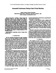
Another way to design the server is to use applications deMATLAB Workspace Experimentation GUI veloped in PERL to access Model’s f_ini Parameters Simulink (sim_ini file) v_init MATLAB and the standard CGI inEvaluation A terface for the exchange of paInitial c v_in rameters and data between the v_in v_in Modified by Read t (......) the User through v_in i c l i e n t a n d t h e s e r v e r. T h e the GUI v MATLAB Web Server software is Simulate e similar to that of ActiveX [28]. X v_out Both solutions are suitable for Write v_out (t,......) v_out environments with pseudo-online or batch simulations: the user reads an exercise in an HTML page, fills in a form with Figure 10. Data interchange between the Java interface and MATLAB/Simulink. the parameters, sends it to the server, and the results are returned as data or graphics environment for analyzing the log of events and actions, [29]; and if the student wants to carry out another experi- avoiding the use of external software. ment with new parameters, these actions must be repeated. The software described herein is currently not available Because the Web-based environment is based on dynamic to the public because it was developed in a research and deand online simulations, the PERL- and CGI-based ap- velopment project for a petrochemical company (see Acproaches have been rejected because of their slowness and knowledgments). The present agreement allows only static character. Instead, we have employed the MATLAB students at our university to use the environment when they API for communication with MATLAB and sockets for the enroll for an automatic control course. Future plans are to data exchange. The use of TCP sockets between the ap- obtain permission to distribute to our students a plets and the server and C routines to communicate with stand-alone release on a CD-ROM and to install an HTTP MATLAB provides a highly flexible solution. Data transmis- server to allow everyone free access to the Web-based exsion to the experimentation applet is carried out in a con- perimentation environment. For information about the softtinuous and sustained way, without the need for ware’s future availability, readers can e-mail the authors. continually starting up CGI routines. Using the GUI and the ideas developed to date, our curAlthough no tool is currently available for coping with de- rent goal is the real-time operation of educational plants lays on the Internet, the use of this network is still consid- (water tanks, heat exchangers, and an inverted pendulum) ered the best solution. To improve real-time access for our through the Internet to provide a remote lab with university students, the Web-based experimentation envi- 24-hour-a-day access. In both cases, MATLAB/Simulink, ronment will be connected by ISDN with the various UNED Java, and C++ will provide the links, closing the loop besupport centers around Spain. In addition, since the server tween the experimental hardware and the applets. The use of video and audio is being considered as anmachine must manage a heavy workload when several students are practicing at the same time (i.e., with several math other way of collecting data from industrial processes. engines running concurrently), we have acquired a Linux Consequently, and as a complement to the 24-hour-a-day box with Pentium III Xeon processors, and use of a high- access, we are developing the hardware and a set of applets s p e e d n e t w o r k w i t h 1 6 L i n u x s y s t e m s r u n n i n g and applications for the remote control of a system composed of a video camera with tilt, focus, pan, and shutter MATLAB/Simulink will be tested in the future. speed.
Additional Goals
Acknowledgments
At present, we are developing a new GUI with two goals in mind: 1) to help the instructor/tutor configure the browsing component by means of the hyperindex contents, and 2) to develop new experiments. In this way, the instructors will not need to know the description syntax of the experiment files and can focus on the design of new experiments. In addition, we are developing new models of plants and new exercises (dc motor, magnetic levitator, etc.) focused on the academic world. An analysis tool will also be added to the
The software described here has its origin in a project between REPSOL-YPF (the largest Spanish petrochemical company) and the UNED Department of Computer Science and Automatic Control. The aim of the project was to create a set of educational materials for the training of operators without a deep knowledge of mathematics. We gratefully acknowledge the support and ideas of the REPSOL-YPF team: J. Acedo, D. Hergueta, F. Cifuentes, and R. González (PETRONOR).
April 2002
IEEE Control Systems Magazine
17
References [1] B. Aktan, C.A. Bohus, L.A. Crowl, and M.H. Shor, “Distance learning applied to control engineering laboratories,” IEEE Trans. Educ., vol. 39, no. 3, pp. 320-326, 1996. [2] S.E. Poindexter and B.S. Heck, “Using the Web in your courses: What can you do? What should you do?” IEEE Contr. Syst. Mag., vol. 19, pp. 83-92, Feb. 1999. [3] K. Maly, H. Abdel-Wahab, C.M. Overstreet, J.C. Wild, A.K. Gupta, A. Youssef, E. Stoica, and E.S. Al-Shaer, “Interactive distance learning over intranets,” IEEE Internet Comput., vol. 1, no. 1, pp. 60-71, 1997. [4] N.A. Kheir, K.J. Åström, D. Auslander, K.C. Cheok, G.F. Franklin, M. Masten, and M. Rabins, “Control system engineering education,” Automatica, vol. 32, no. 2, pp. 147-166, 1996. [5] P. Antsaklis, T. Basar, R. DeCarlo, N. Harris, M. Spong, and S. Yurkovich, “Report on the NSF/CSS workshop on new directions in control engineering education,” IEEE Contr. Syst. Mag., vol. 19, pp. 53-58, Oct. 1999. [6] J.B. Patton and P. Jayanetti, “The making of multimedia power systems control and simulation labware,” IEEE Trans. Educ., vol. 39, no. 3, pp. 314-319, 1996 [Online]. Available: http://www.ece.gatech.edu/users/192/web-use [7] Y. Piguet and D. Gillet, “Java-based remote experimentation for control algorithms prototyping,” in Proc. Amer. Control Conf., San Diego, CA, 1997, pp. 1465-1469 [Online]. Available: http://iawww.epfl.ch/staff/Denis.Gillet/Publications/ACC99.pdf [8] C. Schmid, “A remote laboratory using virtual reality on the Web,” Simulation, vol. 73, no. 1, pp. 13-21, 1999. [9] J. Sánchez, F. Morilla, S. Dormido, J. Aranda, and P. Ruipérez, “Conceptual learning of control by Java-based simulations,” in Proc. IEEE/IFAC Symp. Advances in Control Education (ACE’2000), Gold Coast, Australia, 2000. [10] D. Gillet, C. Salzmann, and P. Huguenin, “A distributed architecture for teleoperation over the Internet with application to the remote control of an inverted pendulum,” in Proc. 2nd Nonlinear Control Network (NCN) Workshop, Paris, France, 2000 [Online]. Available: http://iawww.epfl.ch/Staff/ Denis.Gillet/Publications/NCN2k.pdf [11] T.F. Junge and C. Schmid, “Web-based experimentation using a laboratory-scale optical tracker,” in Proc. Amer. Control Conf. 2000 (ACC’2000), Chicago, IL, 2000, pp. 3463-3467 [Online]. Available: ftp://ftp.esr. ruhr-uni-bochum.de/pub/papers/acc2000RsvlPaper.pdf [12] J.W. Overstreet and A. Tzes, “An Internet-based real-time control engineering laboratory,” IEEE Contr. Syst. Mag., vol. 19, pp. 19-34, Oct. 1999. [13] C. Schmid, “Remote experimentation techniques for teaching control engineering,” in Proc. 4th Int. Scientific-Technical Conference PROCESS CONTROL 2000, Kouty nad Desnou, Czechoslovakia, 2000 [Online]. Available: ftp://ftp.esr.ruhr-uni-bochum.de/pub/papers/Pardubice2000.pdf [14] C.C. Ko, B.M. Chen, J. Chen, Y. Zhuang, and K.C. Tan, “Development of a Web-based laboratory for control experiments on a coupled tank apparatus,” IEEE Trans. Educ., vol. 44, no. 1, pp. 76-86, 2001. [15] M. Johansson, M. Gäfvert, and K.J. Åström, “Interactive tools for education in automatic control,” IEEE Contr. Syst. Mag., vol. 18, pp. 33-40, June 1998. [16] B. Wittenmark, H. Haglund, and M. Johansson, “Dynamic pictures and interactive learning,” IEEE Contr. Syst. Mag., vol. 18, pp. 26-32, June 1998. [17] R.C. Garcia and B.S. Heck, “Enhancing classical control education via interactive GUI design,” IEEE Contr. Syst. Mag., vol. 19, pp. 77-82, June 1999. [18] TOPAS by ACT GmbH [Online]. Available: http://www.act-control.com/ topas.pdf [19] S. Naryanan, N. Rao, J. Geist, P. Kiran, H.A. Ruff, M. Draper, and M.W. Haas, “UMAST: A Web-based architecture for modeling future uninhabited aerial vehicles,” Simulation, vol. 73, no. 1, pp. 29-39, 1999. [20] ECOSimPro by EA International [Online]. Available: http://www. empre.es/ecosim [21] ACSL (Advanced Continuous Simulation Language) by Aegis Technologies Group, Inc. [Online]. Available: http://www.mga.com [22] Scilab Group, Ed., Engineering and Scientific Computing with Scilab. Cambridge, MA: Birkhauser Boston, 1999 [Online]. Available: http://www-rocq. inria.fr/scilab
18
[23] M.A. Hamilton, “Java and the shift to net-centric computing,” IEEE Computer, vol. 29, no. 8, pp. 31-39, 1996. [24] J.L. Weber, Using Java 1.2. Indianapolis, IN: Que, 1998. [25] S. Shirmhammadi, J.C. de Oliveira, and N.D. Georganas, “Applet-based telecollaboration: A network-centric approach,” IEEE Multimedia, vol. 5, no. 2, pp. 64-73, 1997. [26] MATLAB Student Version by The MathWorks, Inc. [Online]. Available: http://www.mathworks.com/products/studentversion/ [27] The MathWorks, Inc., MATLAB External Interfaces, 2001 [Online]. Available http://www.mathworks.com/access/helpdesk/help/pdf_doc/matlab/apiext.pdf [28] MATLAB Web Server by The Mathworks, Inc. [Online]. Available: http://www.mathworks.com/products/webserver/ [29] G.J.C. Copinga, M.H.G. Verhaegen, and M.J.J.M. van de Ven, “Toward a Web-based study support environment for teaching automatic control,” IEEE Contr. Syst. Mag., vol. 20, pp. 8-19, Aug. 2000.
J. Sánchez received his M.S. degree in computer sciences in 1994 from the Polytechnic University of Madrid and his Ph.D. from UNED in 2001. Since 1993, he has been working in the UNED Department of Computer Sciences and Automatic Control as an Assistant Professor. His current research interests are the design of new systems for control education, virtual labs, telepresence, multimedia, and use of the Internet in education. F. Morilla received his degree in physics from the Universidad de Sevilla in 1979 and his Ph.D. from UNED in 1987. In 1983, he joined the UNED Department of Computer Sciences and Automatic Control, where he has worked as an Assistant Professor, an Associate Professor, and since 1998 as a Full Professor of System Engineering and Automatic Control. His current research interests include process modeling, simulation and control, tuning and autotuning of PID controllers, predictive control, and control education. S. Dormido received his M.S. degree in physics from the Universidad Complutense of Madrid (1968) and his Ph.D. degree with a thesis on “Adaptive Sampling” from the University of the Basque Country, Spain, in 1971. In 1981, he was appointed Full Professor of Control Engineering of the UNED Faculty of Sciences. Since 1986, he has been Headmaster of the UNED Department of Computer Sciences and Automatic Control. His scientific activities cover various aspects within the control engineering field: computer control of industrial processes, adaptive systems, model-based predictive control, robust control, and modeling and simulation of continuous processes. J. Aranda received his M.S. degree in physics from the Universidad Complutense of Madrid (1983) and his Ph.D. degree from UNED in 1989. He joined UNED in 1987 as an Assistant Professor, and since 1991 he has been a Senior Professor. His current research interests include applications of hypertext and hypermedia systems to distance teaching, robotic vision systems, and applications to robotic control and flight control.
IEEE Control Systems Magazine
April 2002
Appendix Linking the Java Interface and the MATLAB Workspace In Windows, the communication between the experimentation interface and the calculation engine (i.e., between the Java language and MATLAB) was carried out using the ActiveX Automation protocol. Using the MATLAB-type definition file called mlapp.tlb, located in the folder of the MATLAB distribution code, a group of Java classes and interfaces for wrapping the ActiveX interface with MATLAB can be generated simply and quickly from the MSVJ++ environment. The names of these classes are DIMLApp.class and MLApp.class, and the signatures of the available methods are: public abstract void MinimizeCommandWindow(); public abstract void MaximizeCommandWindow(); public abstract void Quit(); public abstract void GetFullMatrix(java.lang.String, ....., ..... ); public abstract void PutFullMatrix(java.lang.String, ....., ..... ); public abstract java.lang.String Execute( java.lang.String ); Thus, using the methods provided by these classes, the Java code can communicate easily with the MATLAB workspace. The most interesting of the methods is Execute (...). With this method, any MATLAB command can be evaluated in its workspace by means of its argument, and the results of the evaluation can be obtained in the string returned by this method. Once these new nonstandard classes have been generated automatically with MSVJ++, the access to MATLAB/Simulink is immediate. One need only create an instance of an object and operate with it by means of the methods described earlier. In Java code, the creation of an instance in a variable denominated matlab is carried out as follows: import mlapp.*; import com.ms.com.*; ........................... DIMLApp matlab = (DIMLApp) new MLApp(); The peculiarity here is that the class that provides the code with the methods for true access to MATLAB is MLApp, whereas DIMLApp is a Java interface class that describes
April 2002
the syntax or signature of the methods that need to be created for accessing MATLAB through the ActiveX interface. For this reason, the variable matlab, defined as an instance of DIMLApp, is built by using the constructor of the MLApp class, after which the unary operator cast is applied to make an explicit conversion to the DIMLApp class. To further describe the communication process between the two environments, when the instance in the variable matlab is created, MATLAB is opened as a server of the Automation protocol. At that point, it is already possible to command the numerical engine using some of the methods described earlier. For example, to clean the MATLAB workspace from the Java code, it would suffice to include the following sentence: matlab.Execute (“clear all”); To create a vector of five elements, the expression would be: matlab.Execute (“v_out= [ 1, 2, 3, 4, 5]”); or to obtain the value of the variable v_out created in the previous example, the sentence would be: String result = matlab.Execute (“v_out”); Notice that after the operation, the information stored in result would be the same as if, explicitly by means of the keyboard, the vector v_out had been created and evaluated in MATLAB.
Control of Simulink Using the previous methods, total and direct control of Simulink is possible. Since to achieve our goals it was necessary to control different aspects of this simulation environment, a group of generic methods was created with this objective in mind. The methods that have been elaborated for the control of Simulink are shown in detail below. Although the name of each method is sufficiently significant, the functionality of each is described briefly. public void loadSimulinkModel (String MODEL) { matlab.Execute (“open_system (‘” + MODEL + “’)”); } Once MATLAB is open, the above method accomplishes the opening of Simulink and loads the file indicated in the parameter MODEL.
IEEE Control Systems Magazine
19
public void startSimulink (String MODEL) { matlab.Execute (“set_param(‘” + MODEL + “’,’SimulationCommand’,’Start’)”); } Using the above method, the simulation of the model indicated by MODEL can begin. public void stopSimulink (String MODEL) { matlab.Execute (“set_param(‘” + MODEL + “’,’SimulationCommand’,’Stop’)”); } The above method ends the simulation process of the MODEL. public void pauseSimulink (String MODEL) { matlab.Execute (“set_param(‘” + MODEL + “’,’SimulationCommand’,’Pause’)”); } The above method causes the temporary suspension of the simulation process of the MODEL. public void continueSimulink (String MODEL) { matlab.Execute (“set_param(‘” + MODEL + “’,’SimulationCommand’,’Continue’)”); } This last method continues the simulation process of MODEL after a suspension caused by the previous method. These methods are associated with the buttons of the experimentation GUI, so that the user can tailor the evolution of the experiment to his or her observation and analysis capacity. Another use of these controls is to slow the simulation speed by stopping the simulation. This way, students can adjust the simulation to a speed they consider appropriate.
Implementation of the Data Interchange Between the Interface and MATLAB/Simulink The interchange of information between the Java interface and the simulation engine environments begins once the Java application reads the parameters file. This file contains all the parameters for configuring the experimentation interface and the MATLAB workspace so that the student can start the simulation process. The necessary elements for configuring the MATLAB workspace are (see Fig. 10): • v_init Vector: The v_init vector is built with the information in the parameters file and then sent from the
20
Java interface to the MATLAB workspace. This vector includes all the parameters for configuring, a posteriori, the Simulink model: physical parameters of the plant, initial parameters and states of the controllers, initial values of the input variables, sampling rate, etc. • f_ini File: This MATLAB file uses the v_init vector to evaluate a set of functions in the MATLAB workspace to complete the configuration of the model. Although the evaluation of this file produces several lateral effects, the most important result is the creation of a v_in vector in the workspace that constitutes the starting point of the simulation. • v_in Vector: This vector gathers the values of the present elements in the interface (input variables, controller parameters) and transmits them to the simulation process. Thus, it constitutes the linking element between the interface and Simulink. Initially, this vector is constructed from the evaluation of the f_ini file. From then on, the elements of this v_in vector will only change when the user interacts with the GUI or a preprogrammed event takes place. • Model File (sim_ini file): This file contains the Simulink model. Once the v_in vector has been built in the MATLAB workspace, it will already be possible to begin the simulation of the plant, represented by the sim_ini file. This model will send a new v_out vector toward the MATLAB workspace in each step of the simulation. • v_out Vector: The features of the simulation process in Simulink are that in every sampling period, the model reads the v_in vector of the MATLAB workspace, operates with it, and generates a new v_out vector. This vector contains the state of the plant in that sampling rate. The composition of the v_out vector does not vary much from model to model: the first element is time, and the remaining ones are the values of the output variables in that sampling period. Therefore, the values of the v_out vector are visualized in the interface in every sampling period, showing the evolution of the simulation.
It is important to note that the v_out vector is constantly sent to the experimentation GUI, whereas the v_in vector is only delivered to the MATLAB workspace in two cases: when the user modifies a parameter or when some preprogrammed disturbance occurs. This minimizes the information flow between both sides of the environment, which will be a key feature when the local communication channel is replaced with a TCP/IP connection.
IEEE Control Systems Magazine
April 2002