Virtual Metrology Models for Predicting Average PECVD Oxide Film Thickness Ariane Ferreira, Agnès Roussy, Christelle Kernaflen
Dietmar Gleispach, Günter Hayderer
Department of Manufacturing Science and Logistics Ecole Nationale Supérieure des Mines de Saint-Etienne Gardanne, France
[email protected]
austriamicrosystems AG Unterpremstätten, Austria
[email protected]
Hervé Gris, Jérôme Besnard PDF Solutions Montpellier, France
[email protected]
Abstract— The semiconductor industry is continuously facing four main challenges in film characterization techniques: accuracy, speed, throughput and flexibility. Virtual Metrology (VM), defined as the prediction of metrology variables using process and wafer state information, is able to successfully address these four challenges. VM is understood as definition and application of predictive and corrective mathematical models to specify metrology outputs (physical measurements). These statistical models are based on metrology data and equipment parameters. In this paper, some VM models based on industrial data are presented. The objective of this study is to develop a model of the CVD oxide thickness (average) for an IMD (Inter Metal Dielectric) deposition process using FDC data (Fault Detection and Classification) and metrology data. Keywords— Advanced Process Control, CVD Oxide thickness, Partial Least Squares Regression, Tree Ensembles, Semiconductor Manufacturing, Virtual Metrology
I.
INTRODUCTION
The semiconductor manufacturing industry has a largevolume multistage manufacturing system. To ensure high stability and high production yield, reliable and accurate process monitoring is required [1]. Advanced Process Control (APC) is currently deployed for factory-wide control of wafer processing in semiconductor manufacturing. The APC tools are considered to be the main drivers to guarantee a continuous process improvement [2]. However, most APC tools strongly depend on the physical measurement provided by metrology tools [3]. Critical wafer parameters are measured, such as, for example, the thickness and/or the uniformity of thin films. If a wafer is misprocessed in an early stage but detected at the wafer acceptance test, unnecessary resource consumption is unavoidable. Measuring every wafer’s quality after each process step could avoid late wafer scraps but it is too expensive and time consuming. Therefore, metrology, as it is employed for product quality monitoring today, can only cover a small fraction of sampled wafers. Virtual metrology (VM) in contrast enables prediction
of every wafer’s metrology measurement based on production equipment data and previous metrology results [4]-[7]. This is achieved by defining and applying predictive models for metrology outputs (physical measurements) as a function of metrology and equipment data of current and previous steps of fabrication [8]-[10]. Of course it is necessary to collect data from equipment sensors to characterize physical and chemical reactions in the process chamber. Sensor data will constitute the basis for the statistical models that will be developed. A typical Fault Detection and Classification (FDC) system collects on-line sensor data from the processing equipment for every wafer or batch. They are called process variables or FDC data. Reliable and accurate FDC data are essential in VM model [11]. The objective of a VM module is to develop a robust prediction that can provide estimation of metrology and which is able to handle process drifts whether they are induced by preventive maintenance actions or not. This paper deals with the prediction of PECVD (Plasma Enhanced Chemical Vapor Deposition) oxide thickness for Inter Metal Dielectric (IMD) layers using FDC and metrology data. Two types of mathematical models are studied to build VM modules for PECVD processes. Partial Least Squares Regression (PLS) [12]-[13] and a non-linear approach based on Tree ensembles [14]-[16] are considered. The technical challenge and innovation are to build a single robust model, either with PLS or Tree ensembles, which is valid for several products, different layers and two different chucks. The alternative would be to make a model per layer, chuck and product, but we strongly believe that the maintenance of many single models, in our case 12 different models, is not compatible with the constraints of the industry. Section II deals with fabrication process. In section III we present the mathematical background to build VM models. Results and model comparison are described in sections IV. The section V concludes this paper with a summary and a discussion of future work.
II.
FABRICATION PROCESS
The film layer under investigation for thickness modeling is part of the IMD used in the Back-End of Line (BEOL) of a 0.35µm technology process. This oxide layer is used three times during the production of a four metal layer device. PECVD USG (Undoped Silicon Glass) films are commonly used to fill the gaps between metal lines due to their conformal step coverage characteristics. However, as the device geometry is shrinking, the gap fill capability of USG films is no longer sufficient. State of the art technique is the combination of HDP (High Density Plasma) and USG films to provide a highproductivity and low-cost solution. HDP is used to fill the gap just enough to cover the top of the metal line and then the USG is used as a cap layer on top of the HDP oxide film [17].
Wafers are processed in a twin-chamber of a PECVD tool. The same deposition recipe is used for the deposition of different inter-metal layers and several products. During wafer processing, the relevant process parameters that characterize the PECVD process, such as gas flows, pressure, temperature plasma parameters, etc., are gathered. These temporal data are then consolidated with statistical methods. The temporal data (sensors) are collected at a sampling rate of 0.5 second. If too many samples are missing during the data collection, the data are discarded and the wafer is not used in the VM modeling. The temporal data are then transformed into the so-called FDC Indicators. A FDC Indicator is the summarization of temporal data into a single point, based on a given algorithm (mean, range, maximum, minimum, slope, etc). A data set consists of data from production equipment (input data X for VM modeling) and metrology equipment (output data Y for VM modeling). To assure the quality and effectiveness of VM models it is necessary to do preliminary quality studies of process and metrology equipments like variance analysis or repeatability and reliability studies (R&R studies). In addition, context information like layer, product and chuck is essential as categorical input for VM modeling. Input data X consists of 24 indicators and three contextual variables. The output variable Y represents the average of the PECVD oxide thickness of each wafer.
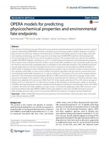
Figure 1: Layer structure for inter metal dielectric
III.
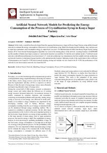
Figure 1 shows the layer structure for one inter metal layer just before the Chemical Mechanical Polishing (CMP) step. The process steps are identical for all three stages. We use identical equipment production recipes, identical metrology setup and identical cleaning procedures for all three stages in the process flow. After metal deposition and structuring (lithography and etch) the HDP oxide is deposited. The HDP oxide film thickness is then measured by ellipsometry, using a 9-site template recipe. FDC data for VM modeling are collected during the USG deposition right after the HDP process. The full oxide stack is measured by the same ellipsometer tool also using a 9-site template recipe. A schematic drawing of the process flow can be seen in figure 2. To guarantee the collection of a proper set of data within a few weeks, ten wafers per lot are measured before and after the USG process. The objective of the VM model is to use the predictive results as an input parameter for the following CMP process step. The CMP tool uses this input data for calculating the polishing time of each wafer and therefore the integrated layer thickness measurement could be skipped. Virtual Metrology
PECVD (HDP)
CMP PECVD (USG) Metrology
Figure 2: Process flow
Metrology
MATHEMATICAL MODELS
A. Notation The following notation conventions are used in this paper: scalars are designated using lowercase italics. Vectors are generally interpreted as column vectors and are designated using bold italic lowercase (i.e. x). Matrices are shown in bold italic uppercase (i.e. X), where xij, with (i=1,…, I) and (j=1,…, p J), is the ijth element of X(I×J). Let X of ℜ be an input data
set and Y of ℜ be arranged in the following way: m
x1T T x X = 2 M xT I
where
y1T T y Y = 2 M yT I
xiT = (xi,1,K ,xi,p ) and yiT = ( yi,1 ,K ,yi,m ) . The
characters I, J, N, p, q, m and n are reserved for indicating the dimension of vectors and matrices of data. B. VM Modeling There are some important points when designing the mathematical models and a methodology that should be considered. In this section we propose two successive stages to deploy mathematical models in order to build a VM Module for an individual process: 1) Data partitioning: Training set and Test set
Let X (I×p) and Y (I×m) be the available data set (cleaned and normalized) respectively from production and metrology process. The data set partitioning consist in the extraction of two units: a unit of 70% of the data set for the trainingvalidation (training and cross validation) and a unit of 30% of the data set for the test. Let XN (N×p) and YN (N×m) be the training-validation data set, and let Xn (n×p) and Yn (n×m) be the test data set with N+n=I. It is possible to split the available data set in a temporal way (chronological selection) without loss of representativeness. In this case study we have chosen this type of data partitioning before the application of the three mathematical models.
If n is equal to the sample size it is called leave-one-out crossvalidation. The prediction performance of the selected model is estimated using the test data set. The performance indicator is the Test Root Mean Square Error of Prediction (TRMSE) computed on the test data set:
Alternatively, the Kennard-Stone method [15] can be used to perform the data set partitioning. The inputs variables
C. PLS Models Consider a set of historical process data consisting of an (I × p) matrix of process variable measurements (FDC data) X and a corresponding (I × m) matrix of metrology data Y. Projection to Latent Structures or Partial Least Squares (PLS) can be applied to the matrices X and Y to estimate the coefficient matrix B in (1).
domain X of ℜ , p
xiT = (xi,1,K ,xi,p ) is considered for the
Kennard-Stone method. It is a sequential method to select a training set uniformly which covers the entire space of input variables X. The selection criteria use the Euclidean distance.
1 n y − yˆ 2 i TRMSE = 100 × ∑ i n i =1 y i
Yˆ PLS = XBˆ PLS + E
A linear regression model of a given process can be written Y = XB + E
(1)
where X is the matrix of input data, Y is the matrix of output data, B is the matrix of regression coefficients and E is the matrix of errors whose elements are independently distributed with mean zero and variance σ2 [18]-[19]. Linear or non linear regression methods can be applied to the matrices X and Y to compute the coefficient matrix B. The regression model is built in two levels: the Training-validation level with the training-validation data set and the test level with the test data set. The training of models that are linear with respect to their parameters (such as linear regressions, polynomials models) can be performed easily with the traditional leastsquares method, whereas the training of models that are nonlinear with respect to their parameters (such as neural networks) requires more complex methods. More details about the training of mathematical models can be found in [16]. Global approaches to model selection in the trainingvalidation level are Cross-validation [20] and Leave-One-Out, methods for estimating generalization error based on resampling [21]. It is obvious to perform the model selection on the basis of the Validation Root Mean Square Error on the Training-validation data set (VRMSE). The VRMSE is given by equation (2): 1 VRMSE = 100 × N
yi − yˆ i ∑ yi i =1 N
2
1/ 2
(2)
where yi is the measured output value, ŷi is the estimated output value from the model, and N is the size of the training data set. The VRMSE is often used for comparing various models. In n-fold Cross-Validation the data are divided into n subsets of (approximately) equal size. The net is trained n times, where one of the training subsets is left out. Only the omitted subset is used to compute the error criterion of interest.
(3)
where yi is the measured output value, ŷi is the estimated output value from the model, and n is the size of test data set.
2) Mathematical Modeling as:
1/ 2
(4)
where Yˆ is the PLS estimate of the process output Y. PLS modeling consists of simultaneous projections of both the X and Y spaces on low dimensional hyper planes of the latent components. This is achieved by simultaneously reducing the dimensions of X and Y, by seeking q (< p) latent variables which mainly explains covariance between X and Y. Therefore this method is useful to obtain a group of latent variables which explain the variability of both, Y and X. The latent variable models for linear spaces are given by Equations (5) and (6) [12]: PLS
X = TP T + E
(5)
Y = TQT + F
(6)
where E and F are error terms, T is an (I × A) matrix of latent variable scores, and P (p × A) and Q (m × A) are loading matrices that show how the latent variables are related to the original X and Y variables. The sample covariance matrix is XTYYTX. The first PLS latent variable t1 = Xw1 is the linear combination of the X-variables that maximizes the covariance between t1 and the Y space. The first PLS weight vector w1 is the first eigenvector of the sample covariance matrix XTYYTX. After the scores for the first component have been computed, the columns of X are regressed on t1 to give a regression vector:
p1 =
X T t1 T t1 t1
(7)
In NIPALS (Nonlinear estimation by iterative Partial Least Squares) algorithm [13] the second latent variable t2, orthogonal to t1, is calculated from the new matrix of covariance X2TY2Y2TX2, where X2 and Y2 are calculated by the equations (8) and (9):
X 2 = X − t1 p1T
(8)
Y2 = Y − t1q1T
q1 is obtained by regression of the columns of Y in t1, i.e.:
b) Build a fully-grown tree τ, following modified CART algorithm
T
q1 =
t1Y T
t1 t1
Build a bootstrap sample (I × p) Xb and corresponding Yb (I × 1) response
a)
(9)
(10)
The second latent variable is computed by the equation t2=Xw2, where w2 is the first eigenvector of the sample covariance matrix X2TY2Y2TX2, and so on. The new latent vectors or scores (t1, t2,…) and the weight vectors (w1, w2, …) are orthogonal. The final models for X and Y are given by Equations (5) and (6). Latent variable models assume that both the process and metrology data spaces are observed with error and that both are effectively of very low dimension (i.e. non-full rank). The dimension A of the latent variable space is often quite small compared with the dimension of the process data space, and it is determined by cross-validation or some other procedure. Effectively, these models reduce the dimension of the problem through a projection of the high-dimensional X and Y spaces onto the low-dimensional latent variable space T, which contains most of the important information [12]. D. Tree Ensemble Models It has been shown by Breiman et al. [22], in the classification case, that under reasonable assumptions, an ensemble procedure allows getting accurate models. Indeed, if the base model has a low-bias and high variance under some random perturbation of the learning conditions, then aggregating a large family of such models give birth to a lowbias, low variance aggregated model, that is more accurate than the individuals models [15]. To allow such results to hold, it is critical that the individual models are as independently built as possible, while maintaining low bias. Tree base learners, either based on algorithms such as CART [22] or C4.5 [23], are known to have a low bias when fully learned (no pruning) [24]. In order to be able to build families of trees that have a low correlation to one another, from a finite dataset, several methods have been proposed: Bootstrapping the learning set (also known as bagging methods), Random splits, Injecting random noise in the response or building random artificial features as (linear) combinations of the existing ones. All these ideas aim at learning trees that are as uncorrelated as possible. Following [22], we use here a combination of bagging from the base learning set, and random splits as our main ensemble method. Base learners are regression trees, following a modified CART algorithm for tree learning. Given X, a set of (I × p) FDC data, and a corresponding Y (I × m) metrology, and 2 parameters q (random selection among features at the individual split level) and nTrees (number of trees grown and aggregated), the algorithm is as follows: 1.
Iterating over the m responses:
2.
Looping 1 -> nTrees:
3.
i.
randomly selecting q