Virtual Metrology Models for predicting physical ...

Virtual Metrology Models for predicting physical measurement in semiconductor manufacturing A. FERREIRA, A. ROUSSY, L. CONDE Ecole Nationale Supérieure des Mines de Saint-Étienne Center for Microelectronics of Provence Georges Charpak 880 Avenue de Mimet, 13541, Gardanne France

Abstract - The semiconductor manufacturing industry has a large-volume multistage manufacturing system. To insure the high stability and the production yield on-line a reliable wafer monitoring is required. The approach, called Virtual Metrology (VM) is defined as the prediction of metrology variables (either measurable or non measurable) using process and wafer state information. It consists in the definition and the application of some predictive and corrective models for metrology outputs (physical measurements) in function of the previous metrology outputs and of the equipment parameters of current and previous steps of fabrication. The goals of this paper are to present a methodology for VM module for individual process applications in semiconductor manufacturing and to present a case study based on industrial data.

wafer state information [9]. It consists in the definition and the application of some predictive and corrective models for metrology outputs (physical measurements) in function of the previous metrology outputs and of the equipment parameters of current and previous steps of fabrication [2].

I. INTRODUCTION

The semiconductor manufacturing industry has a largevolume multistage manufacturing system. To insure the high stability and the production yield on-line a reliable wafer monitoring is required [5]. The Advanced Process Control (APC) is currently deployed in factory-wide control of Front End Of the Line (FEOL) processing in semiconductor manufacturing. The APC tools are the main ways to ensure a continuous process improvement [10]. However, most APC tools strongly depend on the physical measurement provided by metrology tools. Critical wafers parameters are measured, such as, for example, the thickness or the roughness of the thin films. The physical metrology of critical parameters of wafers quality is performed after each processing step only on monitor wafers that are periodically selected by sampling in production equipment for each lot processing (usually one to four wafers per lot). This approach involves that the production wafer quality between two measures is unknown. When the equipment is out of order and the abnormality is not detected in time, many defective wafers may have been produced before the next measure. This will result in a large amount of wafer scraps and will greatly impact the cost. To overcome this problem, an efficient way is to predict the process quality of every wafer using process parameter data of production equipment without physically conducting quality measures. The approach, called Virtual Metrology (VM) is defined as the prediction of metrology variables (either measurable or non measurable) using process and

Fig. 1. Virtual Metrology after a processing step in current semiconductor manufacturing industry [9].

Of course it is necessary to develop a new generation of sensors to improve the characterization of physical and chemical reactions occurring on the wafer surface during process steps. Their data will constitute the basis for the Statistical and Physical models that will be developed. A typical Fault Detection and Classification (FDC) system collects on-line data from process by sensors equipment for every process run. They are called process variables or FDC data. Some reliable available FDC data are essential in VM model. A first approach is to use VM for an individual process using the preprocess metrology data and the FDC data from the chosen tools that are generally collected in real time for fault detection purposes [8]. Into a factory implementation, VM modules for individual processes can be coordinated with one another for a better prediction quality. Since upstream wafer processing affects results of the current process, the VM module for a particular process step can produce a more accurate prediction of the output by using

related preprocess metrology data (predicted via VM as well as current) of the upstream processes [8]. The objective is to develop a robust prediction that can provide estimation of metrology and which is able to handle process drifts and step function changes induced by preventive maintenance disturbances. There are several methods of prediction including: 1) Linear methods: Multiple Linear Regression (MLR), Principal Components Regression (PCR), Partial Least Square Regression (PLS) [8], [10], [11]. 2) Nonlinear methods: Neural Networks (NN): Simple Recurrent Neural Networks (SRNN), Back Propagation Neural Networks (BPNN), Radial Basis Function Neural Networks (RBFN) [1], [4], [7], [9]. The first aim of this paper is to present a methodology for VM module for individual process applications in semiconductor industries. The second aim of this paper is to present an industrial case study. This paper is organized as follows. The section II contains a general VM module Methodology for individual process. The section III presents an industrial case study. The section IV concludes this paper with a summary and a discussion of future work. II. VM MODULE METHODOLOGY FOR INDIVIDUAL PROCESS

In this section we propose a methodology for VM Module for individual process. The Figure 4 presents the methodology proposed.

Fig. 2. Proposition of VM Module Methodology for Individual Process.

This methodology is composed of three successive stages: - Stage 1: Data Pre-process - The aim of this stage is to assure the quality of the data which will be the inputs of the VM models in the Stage 2. The data pre-process includes three steps: - Step 1: Data Sources - To define pilot unit processes, individual process, technology, family of products. After the definition of the family of products, to select the recipes and its important steps that will be used into VM module

development. The input data of VM models are collected from two sources: sensor data of production equipment (FDC data) and measurements data of metrology equipment. To assure the quality and effectiveness of VM models it is necessary to do preliminary quality studies of process and metrology equipments. It can be the variance analysis, like as gauge capability of process and metrology equipments. In this step the choice of technology, family of products, recipes and equipments with high capability and stability is mandatory. - Step 2: Data Acquisition - To define two raw data sets acquisitions both including the FDC data from production equipment (X) and measurements data from metrology equipment (Y). The two raw data sets can be collected from two different periods of production, between 2 and 6 months, for example. Another alternative is to collect a first raw data set from historical data base of production and a second raw data set from Design of Experiments (DOE). - Step 3: Data Consolidation - To define the pretreatment of the two raw data sets collected during Step 2. This includes performing the data cleaning and the statistical data analysis. Data cleaning includes to identify and to remove the outliers, the missing values and the data from out-ofcontrol production. Statistical data analysis include the data normalization, the data correlation studies and the data reduction. The data reduction methods, as stepwise regression or variable probes, can be used to remove the redundant data and select only the critical variables. Moreover, the multivariate analysis, as principal components analysis, can be used to reduce the quantity of columns of the input matrices, X and Y. After the pretreatment of two raw data sets, we will have two off line input data sets for the Phase 2. The first one will be able to be separated in Training Data Set and Running Data Set to construct the VM prediction models. The second one will be able to be used as a Validation Data Set for comparison and validation of models. - Stage 2: VM Module Development - The aims of this stage are to build different prediction models, to compare them and to validate the best model to perform the VM Module. This stage includes three steps: – Step 4: VM Modelling - To choose the linear and the nonlinear prediction methods. To build each prediction models in two levels: the Training Level with the Training Data Set and the Running Level with the Running Data Set. – Step 5: Models Comparisons - To define the performance indices from the robustness and prediction accuracy criteria. To use the Validation Data set for validation and assessment of the models from Step 4. The goal of this step is to select the best model relative to the performance indices. – Step 6: VM Module - To perform the VM Module with the adjustments of the best model chosen in the Step 5. – Stage 3: VM Module Implementation - The objective of this stage is to define the steps to integrate the VM module from Step 6 of Stage 2 into an industrial environment. This phase includes three steps:

– Step 7: VM Module Tests - The aim of this step is to perform off line tests with off line data from production in order to identify problems of the model stability, the model capability and to evaluate results of model when the process drifts. The goal is to define a prototype for off line VM Module implementation. – Step 8: VM Module in Production - To define architectural guidelines for integration of real time VM Module in an industrial environment. Provide guidelines for the full integration of the VM Module into the Manufacturing System. – Step 9: VM Module Consolidation - To define the Maintenance Policies for the update of real time VM Module.

The process has n runs. The previous equation can be written as [13]:

Y = Xθ + ε

-

III. INDUSTRIAL CASE STUDY

The data which have been used for the analysis are FDC (Fault Detection and Classification) data. They have been collected from Chemical Vapor deposition (CVD) equipment. Five VM algorithms, including two linear models and 3 non linear models are studied and compared in this study. The collected parameters’ mean is the chosen statistical indicator which has been followed. In total we have 23 variables (process parameters’ means) with a total of 192 observations. The input variables are X1, X2,…X22, X23 and represent the process parameter means. The output variable Y represents the thickness of the deposited layer for each of the 192 observations. The purpose of the study is to find a predicted model of the CVD deposited layer thickness. Two kinds of models linear and non linear are studied. The linear models are the multiple regression and the multiple regression with stepwise procedure (steepest descent). The non linear models are neuronal Network models: the Multilayers Perceptrons (MLP-I), (MLP-II) and the Radial Basis Function Network (RBFN). A. The Linear Models The individual process step has q outputs (y), l inputs (u), and p process variables (v). k is the process run index, which represents the processing of a single wafer. z is the lot number when a wafer is measured at the metrology station. Let - uk ∈ ℜ(1×l) are the recipe settings at the start of the run k and l the inputs on process equipment. - vk ∈ ℜ (1×p) are the statistical values of p indicators of process (FDC Data) at the end of run k. - yz is the actual measurement of outputs at the metrology run z. yˆ k ∈ ℜ(1×q) are the predicted values for the outputs at the end of run k. Khan et al. [8] present the process modelling by the following equation:

yk = uk A + vk C + kδ + ε k

Where - A ∈ ℜ(l×q) is the matrix of regression coefficients data from the recipe, - C ∈ ℜ (p×q) is the matrix of regression coefficients of p indicators, - δ ∈ ℜ(1×q) is a vector of average drift rates per run k, and - ε ∈ ℜ(n×q) is a multivariate noise with zero mean and variance σ2.

(1)

-

(2)

θ ∈ ℜ(r×q) is the matrix of unknown parameters to be estimated, (θ θ=[A Cδ δ]t and r=(l+p+1)), X is the matrix of regressor variables ε is the white noise following a normal law with a mean equals to 0 and a variance σ².

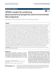
A.1 The Multiple Linear Regression (MR-23) A first multiple regression model has been found using the all 23 input variables X1,…, X23 and the 192 observations. It gives R²adj=50.2%. To improve this model, some non representative observations have been removed. A new model now with only 131 observations gives R²adj=88.94%. For this study the FDC indicators data have been divided into two groups: the first 70% called training data set have been used for the training level and the last 30% called Running data set for the running level. A.2 The Multiple Linear Regression with Stepwise Procedure: Steepest Descent (MR-13) To simplify and to improve the multiple regression model, a steepest descent regression model is applied. Its principle is to remove from the multiple regression model the variable the less significant and to make a new regression with the others keeping variables. This will be done until getting a model using only the significant variables. In this study over the 23 variables 13 have been found significant. Again 70% of these variables have been used for the training level and 30% for the running level. This regression model using 13 significant input variables gives R²adj=85.88%. B. Non-linear Models The non-linear models which are used here are neural network models. For VM models, two types of models are presented: the Multilayers Perceptron Models (MLP-I and MLP -II) and the Radial Basis Function Neural Network (RBFN). The Figure 3 shows an example of a neural network with one input layer with 7 variables, a hidden layer with 3

variables and an output layer with one variable, the target. The goal is to adjust the weight of the input and hidden variables to be able to give the best prediction which is the closest from the target.

been used for the training level and the last 30% for the running level. The studied neural network presents an input layer with 23 neurones (process parameters’ means), a hidden layer with m neurones and an output layer with one neurone (on this case the thickness) B.2 Multilayers perceptron MLP-II The method is the same as described above but in this case not all the input variables are used but only the significant ones: here, 13 variables [6]. The network architectures are illustrated table I. B.3 The Radial Basis Function Neural Network (RBFN)

Fig. 3. Neural Network example.

B.1 Multilayers perceptron MLP-I Feedforward Multilayer Networks with sigmoid nonlinearities are often called Multilayer Perceptrons (MLPs) [6]. The Multilayer Perceptron Model is based on the product between the input vector x and the parameter vector w called the weight. A bias is also added and an activation function is used to find out the output Y.

Y = f (x.w + b )

(3)

The activation function must be strictly no decreasing and bounded. The functions the most often used are the linear function, the hyperbolic tangent and the sigmoid function. In this paper, we are interested in a class of feedforward neural networks: the MLP network with a single layer of hidden neurons with a sigmoid activation function, and a linear output neuron. The output of that network is given by a nonlinear function of its inputs and parameters [6]: Nc   n  n g (x, w ) = ∑  wN c +1,i tanh  ∑ wi , j x j  + ∑ wN c +1, jx j (4) i =1   j =0  j = 0 

Where x is the input (n+1) vector, and w is the vector of (n+1)Nc+(Nc+1) parameters. Hidden neurons are numbered from 1 to Nc, and the output neuron is numbered Nc+1. The parameter wi,j is assigned to the connection that conveys information from input neuron j to neuron i. The input model variables are the process parameters’ means X1, X2,… X22, X23 from FDC. The target is the thickness of the layer after CVD deposition. A set of 131 observations have been used: 70% of the observations have

The RBFN typically have three layers: an input layer, a hidden layer with a non-linear RBFN activation function and an output layer. A RBFN network gives a target function global approximation (response) through a linear combination of m local basis functions. The radial basis functions are Gaussian. The target is the linear combination of last connections’ layer weight. Therefore, the output of the network (for Gaussian RBFN) is given by [6]:

  ∑n ( x j − wij ) 2    (5) g (x, w ) = ∑  wNc +1,i exp − j =1 2   2 w  i =1 i    Nc

Where x is the n vector of inputs, and w is the vector of ((n+2)Nc) parameters, hidden neurons are numbered from 1 to Nc, and the

output neuron is numbered Nc+1. C. Results comparaison To compare these VM models, the Mean Error Absolute (MEA) factor has been calculated for each model. The absolute error is the absolute value from the difference between the real and the approximate value.

MEA =

1 n

n

∑ Y − Yˆ i

i

(4)

i =1

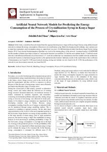
Yi is the real metrology value, Yˆi is the VM model predicted value and n is the number of observations. The MEA calculation results are summarized in the Table I (training step). From the MEA results the Multilayers Perceptron –I is the best model. Its MEA value is the smallest. The Figure 4, part training level confirms this result. The predicted metrology values from MLP-I better fit with the real metrology values.

TABLE I MEA: TRAINING LEVEL VM Models

MEA

Network Architecture (input-Hidden-Output)

Numbers of Parameters

Multiple Regression Multiple Regression with Stepwise Procedure Multilayers Perceptrons -I Multilayers Perceptrons -II Radial function network

0.5313262

NA: Non Available

23

0.8094496

NA

13

from the different models. Then their MEA are calculated to allow us to compare them. The MEA results are illustrated Table II. TABLE I I MEA: VM MODELS’ PERFORMANCES

0.8260405

Network Architecture (inputHiddenOutput) NA:Non Available NA

0.3839831

23-23-1

NA

0.6988438

13-15-1

NA

1.1928393

23-23-1

NA

VM models 0.2915103

23-23-1

NA

0.6861885

13-15-1

NA

1.0876835

23-23-1

NA

Multiple Regression Multiple Regression with Stepwise Procedure Multilayers Perceptron -I Multilayers Perceptron -II Radial basis function network

Thickness mean (Angstroms)

The last step is the selected model performance verification through a test sample. The test sample thickness is predicted

216

MEA

Training level

214

0.5721414

Running level

212 210 208 206 204 202 200 1

8

15

22 29 36 43

50 57 64 71 78

85 92 99 106 113 120 127

Observation number

Thickness m ean (Angstroms)

Actual metrology

216

MR-23

MR-I3

Running level

Training level

214 212 210 208 206 204 202 200 1

8

15

22 29 36 43

50 57 64 71 78

85 92 99 106 113 120 127

Observation number Actual metrology

MLP-I

RBFN

Fig. 4. VM models’ performances (based on 131 observations).

MLP-II

Number of Parameters 23 13

From Table II the MLP-I is again the model which gives the best results with the smallest MEA value of 0.38. The Figure 4, part Running level illustrates the capacity of generalization of the MLP-I model. This model is the one which predicts the best the metrology test sample data. IV. CONCLUSION In this paper a methodology for VM application in semiconductor manufacturing for an individual process has been presented. Different VM models linear and non-linear to predict the CVD deposited thickness layer have been proposed. The comparison of these models showed that the best VM model for the process from Chemical Vapor deposition (CVD) equipment studied here is the non linear neural network: the Multilayers Perceptron. Future works will be able to include: the improvement of the methodology proposed, the definition and improvement of performance indicator to measure robustness and the model accuracy criteria prediction but also, the use of the Validation Data set for validation and assessment of the best model on industrial case studies from semiconductor manufacturing. V. ACKNOWLEDGMENT This work has been done within the framework of HYMNE (High Yield driven MaNufacturing Excellence in sub 65nm CMOS) European IC Manufacturing Industry Project. The authors would like to thank the Advanced Process Control Group of ST MICROELECTRONICS SA, Site Crolles 300, for providing the raw data used in this paper.

REFERENCES [1] Y.-J. Chang, Y. Kang, C.-L. Hsu, C.-T. Chang and T.Y. Chan. “Virtual Metrology Technique for Semiconductor Manufacturing”. Proceedings of the Conference on Neural Networks Sheraton Vancouver Wall Center Hotel, 2006, pp. 5289–5293. [2] P.H. Chen, S. WU, J. Lin, F. Ko, H. Lo, J. Wang, C.H. Yu and M.S. Liang. “Virtual Metrology : A solution for wafer to wafer advanced process control”. Proceedings of the IEEE International Symposium on Semiconductor Manufacturing, September 2005, pp.155–157. [3] F.-T. Cheng. “Researching Strategy and Development Proposal of eManufacturing”. Automation Division of National Science Council, Taiwan, R.O.C, October 2004. [4] F.-T. Cheng, H.-C. Huang and W.-M. Wu “Dual-Phase Virtual Metrology Scheme”. IEEE Transactions on Semiconductor Manufacturing, n. 20, vol. 4 , November 2007, pp. 566–571. [5] A.C. Diebold. “Overview of metrology requirements based on the 1994 National Technology Roadmap for semiconductor”. Advanced Semiconductor Manufacturing Conference and Workshop 1995. ASMC 95 Proceedings. IEEE/SEMI 1995, November 1995, pp. 50–60. [6] G. Dreyfus. Neural Networks Methodology and Applications. Hardcover, 2002. [7] M.-H. Hung, T.-H. Lin, P.H. Chen and R.-C. Lin. “A novel virtual metrology scheme for predicting CVD thickness in semiconductor manufacturing”. IEEE/ASME Transactions on Mechatronics, n. 12 vol. 3, June 2007, pp. 364–375. [8] A.A. Khan, J.R. Moyne and D.M. Tilbury. “An Approach for factory-wide control utilizing virtual metrology”. IEEE Transactions on

semiconductor Manufacturing, n. 20 vol.4, November 2007, pp. 364– 375. [9] T.-H. Lin, M.-H. Hung, R.-C. Lin and F.-T. Cheng. “A virtual metrology scheme for predicting CVD thickness in semiconductor manufacturing”. Proceedings of the 2006 IEEE International Conference on Robotics and Automation, May 2006, pp. 1054–1059. [10] J.R. Moyne. “Making the move to fab-wide APC”. Solid State Technology, n. 47, vol. 9, September 2004, pp. 47. [11] S.J. Qin, G. Cherry, R. Good, J. Wang and C.A. Harrison “Semiconductor manufacturing process control and monitoring : A fabwide framework”. Journal Process Control, n. 16, vol. 3, 2006, pp. 179– 191 . [12] Y.-C. Su, T.-H. Lin, F.-T. Cheng and W.-M. Wu. “Accuracy and RealTime Considerations for Implementing Various Virtual Metrology Algorithms”. IEEE Transactions on Semiconductor Manufacturing, n. 21, vol. 3, August 2008, pp. 426–434. [13] A. C. Rencher. “Methods od multivariate Analysis”. Hardcover 2002.