Virtual Vocalization Stimuli for Investigating Neural ... - CiteSeerX

J Neurophysiol 95: 1244 –1262, 2006. First published October 5, 2005; doi:10.1152/jn.00818.2005.

Innovative Methodology

Virtual Vocalization Stimuli for Investigating Neural Representations of Species-Specific Vocalizations Christopher DiMattina1 and Xiaoqin Wang1,2 1

Laboratory of Auditory Neurophysiology, Departments of Neuroscience and 2Biomedical Engineering, The Johns Hopkins University School of Medicine, Baltimore, Maryland

Submitted 4 August 2005; accepted in final form 29 September 2005

DiMattina, Christopher and Xiaoqin Wang. Virtual vocalization stimuli for investigating neural representations of species-specific vocalizations. J Neurophysiol 95: 1244 –1262, 2006. First published October 5, 2005; doi:10.1152/jn.00818.2005. Most studies investigating neural representations of species-specific vocalizations in nonhuman primates and other species have involved studying neural responses to vocalization tokens. One limitation of such approaches is the difficulty in determining which acoustical features of vocalizations evoke neural responses. Traditionally used filtering techniques are often inadequate in manipulating features of complex vocalizations. Furthermore, the use of vocalization tokens cannot fully account for intrinsic stochastic variations of vocalizations that are crucial in understanding the neural codes for categorizing and discriminating vocalizations differing along multiple feature dimensions. In this work, we have taken a rigorous and novel approach to the study of species-specific vocalization processing by creating parametric “virtual vocalization” models of major call types produced by the common marmoset (Callithrix jacchus). The main findings are as follows. 1) Acoustical parameters were measured from a database of the four major call types of the common marmoset. This database was obtained from eight different individuals, and for each individual, we typically obtained hundreds of samples of each major call type. 2) These feature measurements were employed to parameterize models defining representative virtual vocalizations of each call type for each of the eight animals as well as an overall species-representative virtual vocalization averaged across individuals for each call type. 3) Using the same feature-measurement that was applied to the vocalization samples, we measured acoustical features of the virtual vocalizations, including features not explicitly modeled and found the virtual vocalizations to be statistically representative of the callers and call types. 4) The accuracy of the virtual vocalizations was further confirmed by comparing neural responses to real and synthetic virtual vocalizations recorded from awake marmoset auditory cortex. We found a strong agreement between the responses to token vocalizations and their synthetic counterparts. 5) We demonstrated how these virtual vocalization stimuli could be employed to precisely and quantitatively define the notion of vocalization “selectivity” by using stimuli with parameter values both within and outside the naturally occurring ranges. We also showed the potential of the virtual vocalization stimuli in studying issues related to vocalization categorizations by morphing between different call types and individual callers.

Early studies as well as more recent investigations of the neural representation of species-specific vocal communication sounds in primates and several other species have typically involved playing individual vocalization exemplars or “to-

kens” and recording the elicited neural responses (Cohen et al. 2004; Newman and Wollberg 1973; Rauschecker et al. 1995; Romanski and Goldman-Rakic 2002, 2005; Tian et al. 2001; Wang et al. 1995; Winter and Funkenstein 1973; Wollberg and Newman 1972). Although this approach based on token vocalizations has provided useful insights, it cannot fully elucidate the neural representations of species-specific vocalizations for two important reasons. First species-specific vocalizations are usually composed of multiple acoustical features. Unlike the behaving organism, which processes vocalizations as perceptual units, individual neurons within a particular brain structure are often responsive to particular vocalization features or combinations of features. Therefore one must be able to manipulate all of the vocalization features to determine which features or feature combinations are responsible for driving neural responses. This cannot be easily achieved using traditional filtering techniques. Second, species-specific vocalizations are by their nature stochastic and have intrinsic statistical variations for each call type and caller. Understanding the neural representation of any class of vocalizations requires that we understand the relationship between the neural responses and the intrinsic statistical variations in the vocalizations (Wang 2000; Weiss et al. 2001). The use of vocalization tokens prevents us from fully probing within and outside the natural boundaries of acoustic features of vocalizations. And finally, the results of studies using tokens may in fact depend on the choice of exemplars. As research in human speech processing has demonstrated (Liberman 1996), a more powerful approach is to synthesize de novo statistically accurate vocalization stimuli that allow arbitrary manipulations of their information-bearing parameters (see Suga 1992; Wang 2000). By relying on statistical analysis of the acoustical features from a large number of vocalization samples taken from different call types and multiple individuals, it is possible to synthesize a “virtual vocalization” stimulus that represents a naturalistic or unnaturalistic signal and to arbitrarily manipulate any features of synthesized vocalization stimuli as the experimenter wishes. This will enable a much more detailed and rigorous exploration of principles underlying neural processing of vocalizations than has been possible using tokens, such as the notion of neural “selectivity” to types and callers of vocalizations. Although advanced signal-processing methods like filter bank decompositions and independent components analysis are useful and complementary approaches

Address for reprint requests and other correspondence: X. Wang, Dept. of Biomedical Engineering, The Johns Hopkins University School of Medicine, 720 Rutland Ave., Ross 419, Baltimore, MD 21205 (E-mail: [email protected]).

The costs of publication of this article were defrayed in part by the payment of page charges. The article must therefore be hereby marked “advertisement” in accordance with 18 U.S.C. Section 1734 solely to indicate this fact.

INTRODUCTION

1244

0022-3077/06 $8.00 Copyright © 2006 The American Physiological Society

www.jn.org

Innovative Methodology VIRTUAL VOCALIZATION STIMULI

for neural coding studies (Averbeck and Romanski 2004; Nagarajan et al. 2002; Theunissen and Doupe 1998), one major advantage of parametric natural stimuli is that the dimensions that are used to describe these stimuli are not abstract mathematical dimensions that may not directly correspond to behaviorally relevant features but instead are more intuitive dimensions corresponding directly to the acoustical features in the signal. The approach of using parametric synthetic vocalization stimuli in studying the representations of species-specific vocalizations has been highly successful in elucidating neural processing mechanisms in echolocating bats (O’Neil and Suga 1979; Suga 1988; Suga et al. 1979). The inability of researchers to synthesize and manipulate complex primate vocalizations has partially contributed to slower progress in studies of vocalization processing in nonhuman primates. In this study, we have developed a method for developing statistically accurate parametric virtual vocalization models for the four major call types of the common marmoset (Callithrix jacchus), a highly vocal New World primate. Vocal communication is essential for the marmoset to survive in its natural habitat, and this small primate species remains highly vocal in captivity (Epple 1968). We chose to develop the virtual vocalization stimuli for the four major call types of the marmoset, as they are most frequently used vocalizations in the captive colony. The majority, but not all, of the vocalization types produced by the marmoset are tonal in nature, but tonal vocalizations are not at all idiosyncratic to the marmoset. Several other primate species commonly used in neurophysiology and behavioral studies also have numerous tonal vocalizations of known behavioral relevance, including the macaque monkey, the cotton-top tamarin, and the squirrel monkey (Cohen et al. 2004; Miller et al. 2001a,b; Newman and Wolberg 1973; Romanski et al. 2005; Tian et al. 2001). In addition, the social communication calls of numerous other species of animals studied in auditory neuroscience are largely tonal in nature, including cats and several species of rodents, bats, birds, and frogs (Gehr et al. 2000; Geissler and Ehret 2004; Kanwal et al. 1994; Klug et al. 2002; Liu et al. 2003; Margoliash 1983; Ryan 2001; Suta et al. 2003). In addition to our choice of a highly vocal primate species, the novelty of our approach lies in our detailed statistical characterization of the vocalizations based on a large database of marmoset vocalizations from multiple animals (Agamaite 1997; Agamatie and Wang 1997). We believe that such a detailed analysis is essential for developing statistically accurate synthetic vocalizations and that in principle this general methodology could be applied to numerous other model systems. METHODS

Acquisition and classification of vocalization data Vocalization data used in this study was recorded from eight common marmosets (4 male, 4 female) over a 15-mo period. The subjects were housed in individual cages within a colony room of ⬎20 marmosets and frequently engaged in vocal exchanges with the other marmosets in the colony, most of them housed in family cages. This housing arrangement ensured that vocalizations produced by each subject be uniquely identified from acoustic recordings. Directional microphones (AKG C1000 S) were aimed toward a specific individJ Neurophysiol • VOL

1245

ual, and the microphone output signals were amplified (Symetrix SX 202) and recorded using a two-channel professional digital audio tape recorder (Panasonic SV-3700) sampling at 48 kHz. Recording sessions typically lasted for 4 h and were conducted three times a week. In each recording session, two or four microphones were used with each microphone pointed at a single marmoset. Although most recordings were conducted with the marmosets in their home cages, a limited number of recordings were performed on marmosets temporarily housed in an acoustically shielded cage encapsulated by 3-in Sonex foam (Acoustical Solutions) located within the colony room to minimize the effects of colony noise. Recorded calls were re-sampled at 50 kHz and screened via a real-time spectrographic analyzer (RTS, Engineering Design, Bedford MA) concurrent with audio replay through headphones. Calls from specific individuals were identified based on intensity differences between two recording channels reflecting the aiming of the directional microphones. Vocalizations from those target individuals that were not contaminated with excessive noise or simultaneous vocalizations from other animals were captured and stored on the hard disk of the computer, along with the silent intervals that precede and follow the call. The classification of vocalization samples into call type categories was qualitative and based on the visual similarity of their spectrograms to the spectrograms of previously defined marmoset call types (Epple 1968). An observed call distinctly dissimilar to all previously defined call types was identified as a new call type if it was uttered by at least two monkeys and observed during at least two recording sessions. Apart from being given a unique call identifier, each call was classified as simple or compound. Simple calls are basic acoustical elements uttered either as a complete call or as a discrete syllable in a call. Compound calls are sequences of simple calls with an inter-syllable interval ⬍0.5 s.

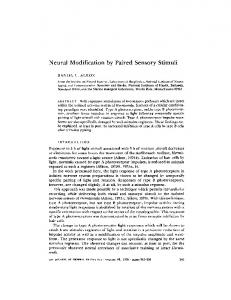
Major call types of the common marmoset Overall, 12 simple call types were identified from 9,772 simple call samples obtained from eight animals (Agamaite 1997). Of these 12 call types, 4 types were produced most frequently, accounting for ⬃75% of the vocalization samples and thus considered to be the major call types of the common marmoset. Exemplars of each one of these four call types are shown in Fig. 1. We focus our efforts on the characterization and modeling of these call types in the present study. The twitter call (Fig. 1A) is composed of a series of 3–15 rapidly ascending upward FM sweeps (referred to as “phrases”) uttered at regular 100- to 150-ms intervals. These sweeps are roughly piecewise linear, and their bandwidth varies as a function of temporal position in the call. The twitter call is an important social communication call, frequently uttered in marmoset vocal exchanges. The trill call (Fig. 1B) is typically 250 – 800 ms in length and uttered at low intensities. The most salient feature of the trill call is a sinusoidal FM, or “trilling,” having a modulation rate of ⬃30 Hz. This sinusoidal FM is often accompanied by amplitude envelope modulation at the same frequency. The phee call (Fig. 1C) is a long (0.5–2.0 s) tonal call, which can vary in intensity from a faint whistle to a very loud scream. Phees usually start with a short upward FM sweep that transitions in to a long flat or gradually ascending FM sweep. The call either terminates with an abrupt cessation of the long flat sweep or more often a rapid descending FM sweep. Although the frequency-time profile for phee calls is quite regular, the amplitude-time profile shows substantial variability from production to production. The phee is commonly uttered as an isolation call. Finally, the trillphee call (Fig. 1D) is essentially a trill call that transitions into a phee call. The trillphee is similar in duration to the phee call and uttered at the same intensity range as phee calls. The transition point from the trill segment typically occurs in the first 60% of the call. We did not observe any calls from our colony that transition from phee to trill.

95 • FEBRUARY 2006 •

www.jn.org

Innovative Methodology 1246

C. DIMATTINA AND X. WANG

A

B

Twitter

Trill

Amplitude

1 0

Frequency (kHz)

-1 20

10

0 0

C

0.2

0.4

0.6

0.8

Phee

0

0.1

D

Trillphee

0.2

0.3

0.4

0.5

0.4 0.6 Time (sec)

0.8

1

Amplitude

1 0

Frequency (kHz)

-1 20

10

0 0

0.4

0.8 Time (sec)

1.2

0

0.2

FIG. 1. Exemplars of the 4 major call types produced by the common marmoset monkey. Both amplitude and spectrographic representations are shown. A: twitter call is a social call composed of a series of upward FM sweeps (“phrases”) uttered at ⬃7 Hz. B: trill call is a brief social call characterized by sinusoidal frequency modulations and in many cases amplitude modulations at ⬃30 Hz. C: phee call is a long contact call comprised of a slow, upward FM, and an irregular envelope. D: trillphee call is a trill call that transitions into a phee.

Acoustical synthesis methodology Each of these four major call types are well described acoustically by a sum of harmonically related frequency and amplitude modulated cosines S(t)⫽A(t) cos [2␲兰t0 f(␶)d␶ ⫹ ␪0], where A(t) is the timevarying amplitude, f(t) is the time-varying frequency, and ␪0 is the initial phase. In the present study, only the fundamental and first harmonic are modeled because higher harmonics are either not detectable above background noise or lie above our recording system Nyquist frequency of 24 kHz, which approximates the upper limit of frequency representation in the primary auditory cortex of this species ( Aitkin et al. 1986). We define our vocalization signal mathematically as S共t兲 ⫽ S1共t兲 ⫹ S2共t兲

(1)

where S(t) is the vocalization signal, S1(t) is the fundamental component, and S2(t) is the first harmonic. Both the fundamental and first harmonic are expressed as the product of an envelope A(t) and a carrier F(t) S 1共t兲 ⫽ A1共t兲F1共t兲

(2)

S 2共t兲 ⫽ A2共t兲F2共t兲

(3)

F1(t) is a cosine oscillator having time-varying instantaneous frequency f1(t), and F2(t) is a cosine with time-varying instantaneous frequency 2f1(t). To define F1(t) mathematically, we first write the general form of a cosine oscillator F 1共t兲 ⫽ cos 关␪共t兲兴

(4)

The instantaneous frequency of an oscillator written in this form is given by the time derivative of the instantaneous phase function ␪(t). For instance, in the simplest case of an oscillator with constant J Neurophysiol • VOL

frequency ␻, the instantaneous phase function is ␪(t) ⫽ ␻t, and its time derivative is the constant ␻. Therefore to obtain an oscillator having time-varying frequency f1(t), we define ␪(t) as the time integral of the instantaneous frequency contour f1(t) after first converting from hertz to radians by ␻1(t) ⫽ 2␲f1(t) ␪ 共t兲 ⫽

冕

t

␻1 共␶兲d␶

(5)

0

⭸ ␪ 共t兲 ⫽ ␻1共t兲 ⫽ 2␲f1共t兲 ⭸t

(6)

Therefore to define a parametric model of a vocalization, we simply need to define the time-varying frequency f1(t) of the fundamental as well the envelopes A1(t) and A2(t) of the fundamental and first harmonic and their relative amplitudes. In the following text, we outline the methods used to extract the time-varying frequency and amplitude contours from the raw data, and the equations used to mathematically describe the acoustical features present in the calls.

Amplitude and frequency contour extraction To eliminate background noise from the colony, a high-pass filter (zero-phase 3rd-order Butterworth, 3-kHz cutoff) was applied to all call samples, which are then converted into a spectrographic representation. It is from this spectrographic representation that most of the measurements are taken. To generate the spectrographic representation for the trill call (Fig. 1B), a 512-point (2 ms) fast Fourier transform (FFT) with a 384 point (75%) overlap was applied to consecutive time segments of the call. From the spectrographic TRILL, PHEE, AND TRILLPHEE CALLS.


www.jn.org


representation, we extracted the amplitude and FM contours of the fundamental component by finding at each time point the frequency in the FFT having the largest amplitude. Hence we get the timeamplitude contour A1(t) and time-frequency contour f1(t) of the fundamental component. This creates two new signals having sampling periods of ⌬t ⫽ 2.56 ms, or equivalently a sampling rate of 390.63 Hz. The corresponding Nyquist frequency (195.31 Hz) is well above most of the spectral energy in the trill call time-frequency and time-amplitude contours. A 512-point FFT window results in spectral resolution of 97.66 Hz, which is adequate to measure the frequency depth modulations in the trill call. The processing of the trillphee (Fig. 1D) and phee (Fig. 1C) calls is identical to that of the trill, with the exception of the size of the FFT window, which is set to 1,024 points in both cases. This longer FFT window gives better frequency resolution which allows us to detect the shallow sinusoidal FM present in the trillphee call as it transitions from trill-like to phee-like character. Once we obtain the amplitude envelope and instantaneous frequency of the fundamental, we measure these features from the first harmonic by finding the spectrogram frequency having the maximum amplitude at each time while restricting our frequency search to the 1 kHz frequency range defined by 2 f1(t) ⫾ 500 Hz. From this measurement we obtain the time-varying frequency contour f2(t) of the first harmonic, as well as its time-varying envelope A2(t). After we have extracted the raw time-frequency and time-amplitude contours from each of the call samples, we can then measure from these contours the values of the parameters that define our model. TWITTER CALL. The twitter call (Fig. 1A) differs from the other three major call types inasmuch as it exhibits a multi-phrase structure,

1247

consisting of a series of rapid upward FM sweeps known as phrases, which are produced at a highly regular inter-phrase interval. From each twitter sample, phrases are extracted from the signal by low-pass filtering the absolute value of the twitter time-amplitude waveform and finding peaks and troughs of the resulting waveform. Each phrase is then converted into a spectrographic representation using a 256point FFT window with a 192-point (75%) overlap, giving us a temporal resolution of ⬃1.3 ms. This high temporal resolution is desirable for this call type with its abrupt frequency transitions and fast amplitude modulations. On conversion to a spectrographic representation, the frequency and amplitude contours of the both the fundamental component and the first harmonic were extracted as for the other call types.

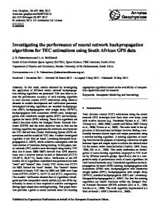
Call model definitions and feature measurement Here we describe the parameters and equations that define the models, and we briefly mention how they are measured from the vocalization samples. The main defining model parameters are shown in Fig. 2 and listed in Table 1, and all parameters measured from the vocalizations are listed in Table 2. TRILL, PHEE, AND TRILLPHEE CALLS. Due to their acoustical similarity, we were able to develop a single parametric space to describe the trill, phee, and trillphee vocalizations. Because their fundamental components are relatively narrowband compared with the twitter call, we refer to them collectively as the “narrowband” call types in this paper. Having these three distinct call types described within a unified parametric framework is very useful because it allows us to morph

FIG. 2. The main parameters defining the virtual vocalization models of the 4 major call types. Brief descriptions of these main parameters are given in Table 1. A complete summary of all virtual vocalization model parameters is given in Table 2. A–C: trill, phee, and trillphee calls, respectively. D: twitter call.

J Neurophysiol • VOL


www.jn.org

Innovative Methodology 1248 TABLE


1. Definitions of model parameters

All call types A1(t) A2(t) Narrowband calls bAM1(t) bFM1(t) fFM1(t) Twitter calls Nphr fmin fknee

Fundamental envelope Harmonic envelope

f1(t) f2(t)

Fundamental frequency contour Harmonic frequency contour

A21 r21

Harmonic attenuation Harmonic ratio

Slow AM modulation Slow FM modulation FM Trilling Rate

dAM1(t) ttrans dFM1(t)

AM modulation depth Trillphee transition time FM trilling depth

fc MFM1 d

Center frequency Slow FM depth duration

Number of phrases Minimum frequency Frequency of knee

IPI fmax

Inter-phrase interval Maximum frequency

tswp tknee

Phrase sweep time Time of knee

Description of the main vocalization model parameters illustrated in Fig. 2.

among them in a continuous manner. The main parameters defining the narrowband call types are illustrated in Fig. 2, A–C. Modeling the frequency contours. Descriptively, the frequency contour f1(t) is modeled as the sum of a slowly modulated component bFM1(t) and a fast, sinusoidal component sFM1(t), as shown in Eq. 7. The slowly modulated component is characterized by its modulation depth MFM1, its center frequency fc, and its trajectory shape given by the normalized function ␤FM1(t) (see Eq. 8). The fast, sinusoidal component sFM1(t) is characterized by its time-varying sinusoidal modulation frequency fFM1(t) and its time-varying sinusoidal modulation depth dFM1(t), as well an initial phase parameter ␪FM1 (Eq. 9). The time-varying FM depth dFM1(t) is the product of the maximum max FM depth dFM1 and a normalized depth function ␦FM1(t) (Eq. 11). We set dFM1(t) to zero for all time points t ⱖ dttrans, where d is the duration of the vocalization and ttrans is the fractional time of transition from trill to phee-like character (Eq. 11). The transition parameter ttrans is set to 0 for phee calls and to 1 for trill calls (Eq. 12). The time-varying modulation frequency fFM1(t) (shown for the trill in the inset of Fig. 3E) can be re-centered to have mean modulation rate fFM1 by simply defining fFM1(t) ⫽ fFM1 ⫹ [fFM1(t) ⫺ ៮fFM1(t)], where ៮fFM1(t) is the mean value of fFM1(t). The frequency contour f2(t) of the first harmonic component is equal to the first harmonic frequency ratio r21 (naturally 2) multiplied by f1(t) (Eq. 13). The FM contour models for all three narrowband call types are summarized in the following text f 1共t兲 ⫽ bFM1共t兲 ⫹ sFM1共t兲

(7)

冉

冊

1 b FM1共t兲 ⫽ MFM1␤FM1共t兲 ⫹ fc ⫺ MFM1 2

冋冋

A 1共t兲 ⫽ bAM1共t兲 ⫺ dAM1共t兲

冋

A2共t兲 ⫽ A21 bAM2共t兲 ⫺ dAM2共t兲

fFM1 共␶兲 d␶

再

t trans ⫽

再

0 1 x 僆关0,1兴

(15)

t

fAM兵1,2其共␶兲 d␶

(16)

0

d AM兵1,2其共t兲 ⫽

(10)

再

t ⱕ d 䡠 ttrans t ⬎ d 䡠 ttrans

dAM兵1,2其 0

(17)

Due to its phrased structure, we characterize the twitter call with both global and phrase parameters. Global parameters are features that describe aspects of overall call structure that do not vary from phrase to phrase, for instance, the inter-phrase interval. Phrase parameters describe the features of particular phrases. A summary of both global and phrase parameters which define the twitter call model is given in Fig. 2D as well as Tables 1 and 2. We create a representative N-phrase synthetic twitter call from the raw data as follows. For each k-phrase twitter call we analyze, we assign the i-th phrase from the call to one of N bins using linear interpolation according to the formula

TWITTER CALL.

t ⱕ d 䡠 ttrans t ⬎ d 䡠 ttrans

(11)

phee trill trillphee

(12)

f 2共t兲 ⫽ r21 f1共t兲

1 1 ⫹ cos 共␪AM2共t兲 ⫹ ␪FM1 ⫹ ␪AM2 ⫹ ␲兲 2 2

(9)

0

dmax ␦ 共t兲 d FM1共t兲 ⫽ FM1 FM1 0

(14)

␪ AM兵1,2其共t兲 ⫽ 2␲

t

␪ FM1 共t兲 ⫽ 2␲

册册册

1 1 ⫹ cos 共␪AM1共t兲 ⫹ ␪FM1 ⫹ ␪AM1 ⫹ ␲兲 2 2

冕

(8)

s FM1共t兲 ⫽ dFM1共t兲 cos 关␪FM1共t兲 ⫹ ␪FM1兴

冕

the ratio of which was greater than a conservative cutoff of 0.5, we measured the time-varying AM rates fAM{1,2}(t) and the phase shifts ␪AM{1,2} between the AM and FM contours. The time-varying AM rates were very similar to the time-varying FM rate, so in the final models, we set the time-varying AM rates equal to the time-varying FM rate. The phase shifts ␪AM{1,2} were bimodally distributed with modes at 0 and 180°. In the models, we set these phase shifts to the larger mode of 180° (␲ radians). AM depths dAM{1,2}(t) were computed for all samples to ensure that there was no bias toward samples that have stronger modulation and thus greater modulation depths. As with the sinusoidal frequency modulations, we set dAM{1,2}(t) to zero for all time points t ⬎ dttrans. For t ⱕ dttrans, we approximate the time-varying AM depths as a constant dAM{1,2}(t). For all three narrowband call types, normalized “backbone” envelopes bAM{1,2}(t) characterizing slow amplitude modulations were computed by averaging the envelopes of all (time-normalized) samples, which washes out faster amplitude modulations such as the 30-Hz trilling. The harmonic envelope was attenuated relative to the fundamental envelope by a factor A21. The models of both envelopes are summarized by the following equations

(13)

Modeling the amplitude contours. Although phee call envelopes reveal no regular structure, analysis of envelope spectral content revealed that many trill and trillphee samples exhibited sinusoidal amplitude modulations in both the fundamental and harmonic envelopes at the same ⬃30-Hz modulation rate observed in the FM contours. This sinusoidal AM is clearly visible in the call samples shown in Fig. 1, B and D. To quantify these amplitude modulations in the trill and trillphee calls, we computed the envelope power spectrum and computed the ratio of signal power between 20 and 35 Hz (the approximate FM trill range) to all signal power ⬎15 Hz. For samples J Neurophysiol • VOL

bin ⫽

冋冉冊册 N

i k

(18)

The exception to this formula is that the first and last phrases of each twitter are automatically assigned to the first and last bin, respectively. Features measured from a phrase are pooled with those measured from other phrases assigned to the same bin, and features are averaged


www.jn.org

Innovative Methodology VIRTUAL VOCALIZATION STIMULI TABLE

2. Parameter values of real and virtual vocalizations

Parameter

Tag

Description

Real

TABLE

Virtual

2. continued

Parameter

2A. Parameters of Twitter Calls Global parameters Nphr G1 IPI

G2

r21 A21

G3 G4

Phrase parameters fmin

P1–3

Number of phrases Inter-phrase interval (ms) Harmonic ratio Harmonic attenuation Minimum frequency (kHz) Maximum frequency (kHz) Knee frequency

fmax

P4–6

fknee

P7–9

tknee

P10–12

Time of knee

tswp

P13–15

Phrase sweep time (ms)

rAM

P16–18

Relative phrase amplitude

fdom

P19–21

Dominant frequency (kHz)

fmed

P22–24

␣AM1

P25–27

Median frequency (kHz) Envelope temporal asymmetry

9

128 ⫾ 11.8

128

2 ⫾ 0.0039 2 ⫺22.14 ⫾ 3.96 ⫺22.1 8.45 5.55 5.96 13.4 12.5 8.66 0.27 0.39 0.36 0.71 0.76 0.75 44.1 44.7 40.1 0.49 1 0.28 9.67 7.45 6.7 9.57 7.62 6.84 0 ⫺0.01 ⫺0.3

2B. Common Parameters of Narrowband Calls d

C1

Duration (s)

fc

C2

Center frequency (kHz)

MFM1

C3

r21

C4

Slow modulation frequency (kHz) Harmonic ratio

A21

C5

ttrans

C6

fdom ⫺M

C8

Dominant frequency (kHz)

rAM ⫺M

C11

Relative section amplitude

fhi

C13

Highest frequency in signal (kHz)

Harmonic attenuation (dB) Time of transition

0.397 ⫾ 0.14 0.921 ⫾ 0.355 1.15 ⫾ 0.44 6.87 ⫾ 0.79 7.42 ⫾ 0.57 7.6 ⫾ 0.61 0.886 ⫾ 0.528 1.24 ⫾ 0.64 1.39 ⫾ 0.59 2 ⫾ 0.004 2 ⫾ 0.002 2 ⫾ 0.001 ⫺20.34 ⫾ 7.27 ⫺26.4 ⫾ 6.27 ⫺33 ⫾ 6.8 1 0.32 ⫾ 0.15 0 6.8 ⫾ 0.8 7.7 ⫾ 0.5 7.8 ⫾ 0.6 1 ⫾ 0.1 1 ⫾ 0.2 1.2 ⫾ 0.3 7.71 ⫾ 0.87 8.1 ⫾ 0.56 8.3 ⫾ 0.81

Tag

Description

Real

Virtual

2B. Common Parameters of Narrowband Calls (cont.)

9.07 ⫾ 2.65

8.48 ⫾ 0.83 5.56 ⫾ 0.67 6.01 ⫾ 0.53 13.6 ⫾ 1.3 12.8 ⫾ 1.85 8.71 ⫾ 1.4 0.27 ⫾ 0.12 0.38 ⫾ 0.12 0.36 ⫾ 0.15 0.71 ⫾ 0.14 0.74 ⫾ 0.14 0.75 ⫾ 0.16 43.4 ⫾ 18.9 42.4 ⫾ 11.3 42.2 ⫾ 18 0.38 ⫾ 0.21 0.81 ⫾ 0.15 0.28 ⫾ 0.18 10.13 ⫾ 1.26 7.6 ⫾ 0.55 6.89 ⫾ 0.49 9.53 ⫾ 0.84 7.62 ⫾ 0.66 6.88 ⫾ 0.64 0.09 ⫾ 0.27 ⫺0.05 ⫾ 0.32 ⫺0.04 ⫾ 0.32

1249

tfhi

C14

Time of highest frequency (sec)

flo

C15

Lowest frequency in signal (kHz)

tflo

C16

Time of lowest frequency (sec)

fFM1

T1

0.3 ⫾ 0.16 0.71 ⫾ 0.36 0.9 ⫾ 0.42 6.02 ⫾ 0.8 6.74 ⫾ 0.69 6.92 ⫾ 0.51 0.127 ⫾ 0.144 0.078 ⫾ 0.2 0.27 ⫾ 0.5

0.27 0.79 1.01 6.35 6.79 6.84 0 0.041 0

2C. Trilling parameters

max FM1

d

T2

DAM1

T3

DAM2

T4

␪FM1

T5

␪AM1

T6

␪AM2

T7

tdmax

T8

min FM1

d

T9

tdmin

T10

mean FM1

d

Mean trilling frequency (Hz) Maximum FM trilling depth (kHz) AM1 modulation depth AM2 modulation depth Initial FM phase AM1-FM1 phase shift AM2-FM1 phase shift Time of Maximum FM depth (sec) Minimum FM depth (kHz) Time of Minimum FM Depth (s) Mean FM depth (kHz)

T11

27.1 ⫾ 1.6 27.8 ⫾ 2.2 0.913 ⫾ 0.32

27.13 28 0.97

0.5 ⫾ 0.19

0.52

0.46 ⫾ 0.12 0.4 ⫾ 0.11 0.54 ⫾ 0.16 0.4 ⫾ 0.12 3.07 ⫾ 1.54 3.08 ⫾ 1.4 2.98 ⫾ 0.28 2.9 ⫾ 0.5 3.12 ⫾ 0.25 3.03 ⫾ 0.42 0.194 ⫾ 0.153 0.074 ⫾ 0.08 0.35 ⫾ 0.16 0.2 ⫾ 0.1 0.136 ⫾ 0.14 0.18 ⫾ 0.14 0.587 ⫾ 0.176 0.36 ⫾ 0.12

0.48 0.41 0.58 0.42 ␲ ␲ ␲ ␲ ␲ ␲ 0.215 0.04 0.39 0.2 0 0 0.59 0.34

2D. Sample Sizes ALL M335 M363 M0087 M60107 M284 M79 M70100 M358

0.406 0.87 1.18 6.82 7.46 7.59 0.87 1.09 1.38 2 2 2 ⫺20.4 ⫺25.4 ⫺32.8 1 0.31 0 6.8 7.7 7.9 1 1.2 1.22 7.62 8 8.3


Twitter 1080 Trill 1000 Phee 1504 Trillphee 480

180 288 476 95

253 188 193 60

145 305 409 328

172 206 230 75

264 199 367 475

257 254 188 79

193 292 203 205

135 125 226 122

Acoustical parameters measured from vocalization samples are listed in the fourth column (Real). Corresponding parameter values assigned to virtual vocalization models are listed in the fifth column (Virtual). Parameters that were not explicitly specified in the model definition were measured from synthesized vocalizations and listed in italics in the fifth column. Section A is twitter call parameters. The parameter set is divided into global parameters of the call and features measured from individual phrases. In columns 4 and 5 of Phrase parameters (P1–P27), values listed in each represent beginning (B), middle (M) and end (E) sections of a vocalization, respectively. Section B is common parameters measured from the three narrowband call types (trill, phee, trillphee). For fdom and rAM, only the values measured from the middle section (M) are shown due to space limitations. Values of parameter tag C7 ( fdom⫺M), C9 ( fdom⫺E), C10 (rAM⫺B), and C12 (rAM⫺E) are not shown. Section C is “trilling” parameters measured from the trill and trillphee calls. The last section has sample sizes used in the calculations of call type and caller parameter distributions. Parameter values are shown for the representative virtual vocalization of each call type. Free parameter values shown are those specified in the model definitions. Additional (italicized) parameters are measured from the virtual vocalizations post-synthesis.


www.jn.org


Percent Samples

A

C. DIMATTINA AND X. WANG Twitter Phee Trill Trillphee

60

B

15

40

10

20

5

0 1.95

2

0 -60

2.05

Harmonic Ratio

Percent Samples

C

D

15

10

5

5

0.5

1

1.5

2

2.5

5

FM Rate (Hz)

20

FM AM

30

15

F

FIG. 3. Distributions of selected vocalization parameters. A: frequency ratio of the 1st harmonic to the fundamental (r21) for all call types. B: attenuation of the 1st harmonic relative to the fundamental (A21) for all call types. C: call duration (d) for all call types. D: center frequency of the fundamental component (fc) for all call types. E: mean AM and FM modulation or trilling rates for the fundamental component of the trill and trillphee vocalizations (fFM1, fAM1). Inset: averaged time-varying trill call FM rate for all individuals (thin lines) and the mean of all individuals (heavy line). F: trillphee call time of transition (ttrans) from trill-like to phee-like character. Means and SDs of all parameters measured from the calls are shown in Table 2.

10 8

26 22

10

Center Frequency (kHz)

Duration (sec)

Percent Samples

0

0 0

15

-20

15

10

0

E

-40

Harmonic Attenuation (dB)

0

0.4

6

0.8

Time

10

4 5 0

2 15

20

25

30

Modulation Rate (Hz)

35

0

0

0.2

0.4

0.6

0.8

1

Trillphee Transition Time

within bins to determine the phrase parameter values for the representative twitter calls computed for each animal. The four main global parameters are the number of phrases Nphr, the inter-phrase interval IPI, the harmonic ratio r21 (naturally 2) and the harmonic attenuation A21, which we approximate as being constant across phrases. These are illustrated in Fig. 2D. From the frequency contour extracted from the n-th phrase, we measure the starting frequency fmin(n), ending frequency fmax(n), sweep duration tswp(n), and the relative amplitude rAM(n) of the phrase with respect to the other phrases in the call, normalized to the loudest phrase. The time of the “knee” tknee(n), or the fractional point in the phrase at which the FM sweep rate increases abruptly, is accurately estimated by doing an unconstrained fit of a piecewise linear function to the FM contour. The point in time where the two lines join is taken to be the time of the knee for the phrase, and the frequency occurring at this time point is taken to be the knee frequency fknee(n) for the phrase, which is normalized to [0,1] by expressing it as a fraction of the phrase bandwidth bw(n) ⫽ fmax(n) ⫺ fmin(n). Once tknee(n) has been computed, we then measure both frequency and amplitude contours from the phrase relative to the knee time. We do this to minimize the smoothing which occurs when different call samples are averaged together, and we manage to preserve differences between individual animals in the detailed AM and FM shapes of the phrases by doing so (see Fig. 6). For the n-th phrase, we represent both frequency and amplitude contours before the time of knee [fbk(t, n), Abk(t, n)] and J Neurophysiol • VOL

after the time of knee [fak(t, n), Aak(t, n)] for each call by a 25- and 10-dimensional vector, respectively, by assigning frequency-time points taken from all call samples from each animal to the appropriate bin and then averaging within the bins. Each of these contours is expressed as a function from the normalized domain [0,1] to the normalized range [0,1]. Mathematically, the overall virtual twitter signal S(t) is modeled as a sum of Nphr phrases, each of which is composed of both the fundamental and first harmonic

冘

Nphr

S共t兲 ⫽

S1共t,n兲 ⫹

n⫽1

冘

Nphr

S2共t,n兲

(19)

n⫽1

As with the other call types, each of the phrases is modeled as the product of a time-varying amplitude contour and a cosine oscillator having a time-varying frequency. The n-th phrase is given by S 兵1,2其共t,n兲 ⫽

再

A兵1,2其共t,n兲F兵1,2其共t,n兲 0

t 僆关tst共n兲,tsp共n兲兴 otherwise

(20)

1 1 t st共n兲 ⫽ tswp共1兲 ⫹ 共n ⫺ 1兲IPI ⫺ tswp共n兲 2 2

(21)

t sp共n兲 ⫽ tst共n兲 ⫹ tswp共n兲

(22)

In Eqs. 20–22, tst(n) and tsp(n) are the start and stop times of the n-th


www.jn.org


phrase, tswp(n) is the sweep time of the n-th phrase and IPI is the inter-phrase interval. When considering an individual phrase, the time variable is shifted by subtracting the phrase start time, so that the time domain for the n-th phrase is [0, tswp(n)]. The time of knee in this interval is simply k ⫽ tknee(n)tswp(n). The amplitude contours A{1,2}(t,n) and frequency contours f{1,2}(t,n) are defined piecewise by the following expressions

再再

rAM共n兲Abk1共t/k,n兲 A 1共t,n兲 ⫽ rAM共n兲Aak1共共t ⫺ k兲/共tswp共n兲 ⫺ k兲,n兲

0⬍t⬍k k ⬍ t ⬍ tswp共n兲

(23)


(24)

fmin共n兲 ⫹ 关fknee共n兲 ⫺ fmin共n兲兴fbk1共t/k,n兲 fknee共n兲 ⫹ 关fmax共n兲 ⫺ fknee共n兲兴fak1共共t ⫺ k兲/共tswp共n兲 ⫺ k),n兲


(25)

f 1(t,n) ⫽

再

f 2共t,n兲 ⫽ r21 f1共t,n兲

measurements of multiple individual feature dimensions for each call, we defined a metric similar to Mahalanobis distance (Duda et al. 2001) to quantify the statistical distance between a measured parameter vector x ⫽ (x1, . . . , xn) and the mean vector for the parameter space ␮ ⫽ (␮1, . . . , ␮n) obtained by averaging across all sample. It is given by the following expression D ␮共x兲 ⫽

A21rAM(n)Abk2(t/k,n) A21rAM(n)Aak 2((t⫺k)/(tswp(n)⫺k),n)

A 2 (t,n) ⫽

1251

(26)

All of the parameters defining the twitter calls are summarized in Tables 1 and 2.

Analysis of accuracy To verify that these representative virtual vocalizations capture the first-order statistical properties of the natural calls, which they aim to model, we applied feature measurement software to measure various acoustical features from both the ensemble of natural vocalizations as well as the virtual vocalizations. In addition to measuring the parameter dimensions which were used to define the virtual vocalization models, we also measured for each call type a set of additional parameters not explicitly specified in the model definitions. By doing this, we test the accuracy of our models to a greater extent. Here we describe additional acoustical features which were measured from the vocalizations. All parameters measured from the vocalizations, both model parameters and additional parameters, are summarized in Table 2. In addition to the model-defining parameters described in the preceding text, from each of the three narrowband call types (trill, phee, trillphee) the lowest and highest frequencies in the signal and their times of occurrence (fhi, flo, tfhi, tflo) were measured. Each vocalization was then divided into three sections of equal duration for further analysis, which we denote beginning, middle, and end (B, M, E). We took the power spectrum of each section and measured the peak, which we term the section dominant frequency (fdom). The relative amplitude of each call section (rAM) was measured by dividing the mean section amplitude by the mean amplitude for the entire call. For the trill and trillphee calls, we measured four additional parameters that describe the FM trilling observed in these calls. The minimum and maximum FM depths observed in the calls and their min max times of occurrence (dFM1 , dFM1 , tdmin, tdmax) were measured, as well mean as the mean FM depth (dFM1 ). For the twitter call, we took the power spectrum of the beginning, middle and end phrases, and measured fdom as for the other call types. We also measured the median frequency in the phrase FM trajectories (fmed). The twitter phrase envelope shape was quantified by measuring the envelope temporal asymmetry ␣AM1 from the fundamental component of the beginning, middle, and ending phrases. The temporal asymmetry ␣AM1 is an index that tells us the extent to which the envelope of the fundamental component of a twitter phrase is “ramped” (␣AM1 ⬎ 0) or “damped” (␣AM1 ⬍ 0) in the time domain by measuring whether more of the area under the envelope lies in the first or second half of the phrase. All of these additional parameters measured from the vocalizations as well as the defining model parameters are listed in Table 2. MEASUREMENT OF INDIVIDUAL ACOUSTICAL FEATURES.

ACCURACY ACROSS MULTIPLE FEATURE DIMENSIONS. To asses the overall acoustical accuracy of the virtual vocalizations based on our


1 N

冘 N

i⫽1

兩xi ⫺ ␮i兩 ␴i

(27)

Note that this distance measure is simply the absolute value of the z-score averaged across all feature dimensions. This formula provides a simple interpretation of the notion of multidimensional distance and ensures equal weighting of dimensions. We apply this measure not only to the virtual vocalizations but also to every single call sample used to define the virtual vocalization. This enables us to determine which percentage of natural call samples lie at a distance further from the statistical mean than the synthetic mean vocalization. If the synthetic vocalization is indeed a statistically representative example of a given call type produced by a given animal, its feature vector should be at or near the distribution mean and this percentage should be close to 100%. If there is a serious overall discrepancy between the synthetic vocalization and the natural samples, this percentile should be close to 0%.

Comparing neural responses to real and virtual vocalizations Detailed descriptions of the procedures used to prepare marmoset monkeys for electrophysiological recordings appear elsewhere (Lu et al. 2001). Briefly, marmosets were adapted to sit in a primate chair. An aseptic implant surgery was performed to prepare the animal for chronic recordings. A thick cap of dental cement was formed over the skull except for small regions lateral to the lateral sulcus on each side. A thin layer of dental cement was placed over the skull regions overlying the auditory cortex; this enables us to access the underlying brain for electrode recording. Two stainless steel posts were fixed in the thick cap of dental cement to be used for immobilization of the animal’s head during recordings. The animal was monitored carefully for 2 weeks after surgery, and pain relievers and antibiotics were administered as needed.

ANIMAL PREPARATION AND SURGERY.

ELECTROPHYSIOLOGICAL RECORDING PROCEDURES. All recording sessions were conducted within a double-walled, sound-proof chamber (Industrial Acoustics). Daily recording sessions, each lasting 3–5 h, were carried out for several months. The brain was accessed via miniature holes in the skull (diameter: ⬃1 mm) overlying the auditory cortex. These holes were cleaned daily with saline and antibiotics and typically kept open for 1–2 wk before sealing with dental cement. Polyvinylsiloxane dental impression cement (Kerr) was used to seal the recording holes between recording sessions. Single-unit activities were recorded using a tungsten microelectrode of impedance typically ranging from 2 to 5 M⍀ (A-M Systems). For each cortical site, the electrode was inserted nearly perpendicularly to the cortical surface by a micromanipulator (Narishige) and advanced by a hydraulic microdrive (David Kopf Instruments). Action potentials were detected by a template-based spike sorter (MSD, Alpha Omega Engineering) and continuously monitored by the experimenter while data recordings progressed. Signal-to-noise ratio was typically ⬎10:1 (see Lu et al. 2001). The location of the primary auditory cortex was determined by its tonotopic organization, proximity to the lateral sulcus, and general response properties (tone driven with short latency). We did not attempt in this study to estimate unit laminar locations. COMPARISON OF REAL AND VIRTUAL VOCALIZATIONS. To determine the extent to which our modeling strategy is effective at producing stimuli that drive auditory cortex units in a similar manner as natural calls, we made synthetic models of five individual twitter


www.jn.org



call token recordings of exceptionally high quality from one animal. We extracted amplitude and frequency contours from the fundamental and first harmonic of the natural twitter call and then used them to define the amplitude and frequency contours of two harmonically related cosine oscillators. Hence for every one of the five twitter call tokens Ti (i ⫽ 1–5), we synthesize an acoustically matched virtual twitter call Vi. Because the token vocalizations typically contain a small amount of background noise and it is known that in some neurons the presence of background noise can affect neural responses (Bar-Yosef et al. 2002), we also added noise to the virtual vocalizations to match the noise seen in the tokens. This was accomplished by high pass filtering the low-frequency noise from the token (3rd-order Butterworth, 3-kHz cutoff, zero phase), which does not intersect with the twitter call frequency range of 5–25 kHz. Then, 500 point samples of background noise were taken from the beginning of the token and from these samples the SD ␴i of the background noise for that token was estimated. Gaussian white noise having mean 0 and SD ␴i was then added to the virtual vocalization, which was then high-pass filtered with the same filter we applied to the token. This ensured that the noise that lies within the twitter frequency range was approximately the same amplitude in both the natural call and the virtual vocalization. Finally, each real-virtual vocalization pair was matched for overall signal power. To compare responses to the two sets of stimuli (real and virtual), we ran a procedure on a set of units that were found to be twitterresponsive after preliminary tests with virtual vocalization stimuli representing three (twitter, phee, trill) or all four of the major call types. This procedure involved playing a small number of real-virtual vocalization pairs (3 or 5) with a large number of repetitions (ⱖ10, typically 15–20). Using a large number of repetitions enables comparisons between real and virtual vocalization responses for each unit on a call-by-call basis. Stimuli were presented in randomized block fashion with inter-stimulus intervals ⬎1 s. For each real-virtual pair, we apply the Wilcoxon rank-sum test to the spike counts elicited by both stimuli in the pair to see if the unit is being driven similarly by the real and virtual vocalizations.

Vocalization samples were obtained from eight individual marmosets (4 males, 4 females) in a previous study (Agamaite and Wang 1997). Of the 12 simple call types identified, four types accounted for ⬃75% of the recorded samples. We therefore consider these four calls types (the twitter, trill, trillphee, and phee calls, shown in Fig. 1) to be the four major call types produced by this species. In this study, we analyze 7,187 samples of these four types. A breakdown of samples by call type and caller are given in Table 2D.

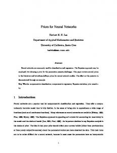
butions of call duration. The trill call has the shortest duration (400 ms on average), while the other three calls have mean durations closer to a second. Notice that there is a substantial variability in call duration for all call types and a high degree of overlap between call types. The three narrowband vocalizations also overlap significantly in fundamental center frequency fc, which is estimated from the call samples by averaging the highest and lowest frequencies present in the fundamental component. This is plotted in Fig. 3D with only the middle phrase shown for the twitter call. In addition to a substantial overlap in center frequency, the three narrowband vocalizations show a substantial overlap in their bandwidth (trill: 1.7 ⫾ 0.7 kHz, n ⫽ 1,000, phee: 1.4 ⫾ 0.7 kHz, n ⫽ 1,504, trillphee: 1.4 ⫾ 0.7 kHz, n ⫽ 480, distributions not shown). Because the major call types show substantial overlap in their harmonic structure, duration, center frequency, and bandwidth, more complex spectral and temporal parameters may be necessary to reliably discriminate these three call types perceptually. Figure 3, E and F, illustrates more complex spectral-temporal parameters specific to two particular call types (trill and trillphee), namely sinusoidal frequency and amplitude modulation or “trilling”. The FM and AM of the fundamental component of the trill and trillphee vocalizations is illustrated in Fig. 3E. For the trill call, the FM measured from all vocalization samples was 27.1 ⫾ 1.6 Hz, and the AM measured from samples showing substantial modulation (see METHODS for criterion) was 26.9 ⫾ 1.7 Hz, and these two variables were well correlated with r ⫽ 0.85. Similarly, the AM in the envelope of the first harmonic was 26.9 ⫾ 1.6 Hz, and this was also well correlated with the FM (r ⫽ 0.83) as well as the AM of the fundamental (r ⫽ 0.84). Similar results were found for the trillphee vocalization, which had a mean FM rate of 27.8 ⫾ 2.2 Hz and a mean fundamental AM rate of 27.4 ⫾ 1.6 Hz. We find that both the AM and FM rates change similarly as a function of time in a nearly linear manner, and in the models, the FM and AM modulation rate contours are set equal. The inset of Fig. 3E shows the FM rate as a function of time for the trill call from each individual animal (thin lines) and averaged over all 8 animals (thick line). Another complex spectraltemporal parameter that enables one to distinguish the trillphee vocalization from the trill and phee calls its fractional transition time ttrans from trill-like to phee-like character (see Fig. 2D). The distribution of this parameter is shown in Fig. 3F. We see from this graph that the transition time typically occurs in the first 2/3 of the vocalization (0.32 ⫾ 0.15).

BUILDING PARAMETER DISTRIBUTIONS. Parameters that describe the main acoustical properties of each call type were measured from the vocalization samples in our database. Figure 3, A–D, shows distributions of some parameters that describe basic acoustical features common to all four call types. For each of the four call types, the frequency ratio r21 of the first harmonic to the fundamental (Fig. 3A) was for all samples nearly identical to 2 with very little variability from exemplar to exemplar. The distribution of attenuation A21 of the first harmonic relative to the fundamental is plotted on a decibel scale for all four call types in Fig. 3B. The degree of attenuation differed somewhat between call types with the trill call showing the least harmonic attenuation [⫺20 ⫾ 7 (SD) dB] and the phee call the greatest harmonic attenuation (⫺33 ⫾ 7 dB). Figure 3C shows distri-

DEFINING NATURALISTIC REGIONS OF PARAMETER SPACE. These parameter distributions computed for each of the vocalization model parameters enable us to define parameter ranges that represent naturalistic vocalization signals for each call type. One can make a vocalization stimulus unnatural along single or multiple parameter dimensions by setting the values of one or more parameters outside of the region of parameter space representing natural vocalization signals. Figure 4 illustrates multidimensional parameter distributions for the twitter and trill calls. Figure 4A shows a plot of two trill call parameters, max the FM rate and maximum FM depth (fFM1, dFM1 ). We draw ellipses at 1, 2, and 3 SDs from the subspace mean of (27.1, 913 Hz). These ellipses enable us to define boundaries between the regions of parameter space representing natural signals and

RESULTS

Measurement of vocalization parameters



www.jn.org


FIG. 4. Vocalization parameter distributions define natural and unnatural regions of vocal parameter space. A: 2-dimensional subspace defined by 2 trill call free parameters: FM trilling rate and maximum FM trilling depth (fFM1, max dFM1 ). Ellipses are drawn at 1, 2, and 3 SDs from the mean. Regions of this parameter space outside of the 3 SD ellipse can be considered to represent unnatural signals. B: 2-dimensional subspace defined by 2 twitter call free parameters: inter-phrase interval and number of phrases (IPI, Nphr).

the regions of space representing un-natural signals. For instance, we can define all points lying outside of the 2 or 3 SD ellipse to represent “unnatural” regions of parameter space, and all points lying within 2 SDs to represent “natural” signals. Similarly, Fig. 4B shows a two-dimensional twitter call parameter subspace consisting of the inter-phrase interval and the number of call phrases (IPI, Nphr). It is easy to see that this process can be extended beyond two dimensions to quantitatively delimit regions of the parameter space that represent natural calls. Synthesizing representative vocalizations Using the model definitions outlined in Fig. 2, together with parameter distributions obtained by measuring acoustical feaJ Neurophysiol • VOL

1253

tures from our database of call samples, we synthesize a representative virtual vocalization of each type for each animal, as well as an overall representative virtual vocalization of each type by pooling data across animals. Figure 5 illustrates the overall synthetic mean vocalizations of each type. These vocalizations can be thought of as representing the “average” or “prototypical” call of that type, and their default parameter values are set at or near the species distributions means as summarized in Table 2. We see that they are qualitatively similar to the exemplars shown in Fig. 1. Although these prototypical virtual vocalizations generated from data from multiple callers shown in Fig. 5 are useful for exploring neural and behavioral representations of vocalization features that are invariant across callers (for instance, the presence of sinusoidal frequency modulations in the trill call or phrase structure in the twitter call), one would also like to be able to explore the representation of individual caller identity. It has been shown previously that vocalizations of a given type produced by different individual callers can be reliably separated along multiple acoustical parameter dimensions (Agamaite 1997; Agamaite and Wang 1997). Therefore we should require the virtual vocalization representative of each individual to be statistically representative of the vocal productions sampled from that individual. More precisely, given the distributions of parameters measured from an individual monkey and a vector of these same parameters measured from that monkey’s representative virtual vocalization, one should find that the vector measured from the representative call lies within the regions of parameter space occupied by that animal’s productions. An example of this concept is illustrated in Fig. 6, where we see the representative virtual twitter vocalizations from two different animals, M363 and M60107 (Fig. 6A). We measure six example parameters from these virtual vocalizations using the same software that we used to extract these parameters from the natural call samples. Figure 6B illustrates a twodimensional parameter subspace consisting of the middle phrase sweep time (tswp) and the temporal asymmetry of the middle phrase envelope (␣AM1⫺M). Figure 6C illustrates a subspace consisting of the middle phrase bandwidth (bw⫺M) and the middle phrase center frequency ( fc⫺M). Figure 6D illustrates the subspace consisting of the inter-phrase interval and the number of call phrases. Ellipses are drawn at 1 SD, with small symbols denoting these parameter values measured from natural samples and large symbols denoting these parameter values measured from the virtual vocalizations. For these two animals, along these dimensions, we see that there is a good degree of separation between the two animals and that the parameter values measured from each of the virtual vocalizations lie within a SD of the statistical means. Deviations from the mean reflect systematic error in the synthesis procedures, and we quantify the accuracy of the synthesis method across all call types and callers in the following section. For this example pair of individuals, we see that along the selected parameter dimensions the virtual twitter vocalization for a particular animal is statistically representative of the call samples from that animal. We further demonstrated using a metric-based classifier procedure (described in the following section) that for each call type the virtual vocalization synthesized for each animal is more statistically representative of the natural samples obtained from that animal than


www.jn.org



A

B

Twitter

Trill

Amplitude

1 0

Frequency (kHz)

-1 20

10

0 0

C

0.4

0.8

0

1.2

D

Phee

0.2

0.4

0.6

Trillphee

Amplitude

1 0

Frequency (kHz)

-1

20

10

0 0

0.4

0.8

1.2

0

0.2

0.4

0.6

0.8

1

Time (sec)

Time (sec)

FIG. 5. The representative virtual vocalizations for each of the 4 major call types. These vocalizations were synthesized using data from all 8 animals and can be thought of as representing the “average” or “prototypical” exemplar of that vocalization category.

samples obtained from the other animals. In other words, the virtual vocalizations preserve the features that define individual vocal signatures. Analysis of acoustical accuracy To quantitatively asses the extent to which the virtual vocalizations are statistically representative of the natural calls, we measured an identical set of parameters from both the natural call samples and the representative virtual vocalization for each call type and animal. Although many of these parameters were specified in the definitions of the virtual vocalizations, several other parameters which were not explicitly specified in the call type definitions (for instance, the vocalization power spectrum peak) were also measured. By measuring additional features not explicitly specified in the models, we can more carefully investigate the accuracy of our virtual vocalization stimuli. All of the individual parameters measured from the virtual vocalizations for comparison with the natural call samples are listed in Table 2 and are shown in italic typeface.

FEATURE MEASUREMENT.

For each parameter, we measure from the virtual vocalizations, we convert it into a z-score using the means and SDs of the distributions of that parameter obtained from the call samples. z-scores along each parametric dimension are plotted in Fig. 7, A and B. For convenience, we separate the parameters we measure into groups. Narrowband call parameters are divided into a set of 16 “common” parameters (Fig. 7A, top), which we measure from all three narrowband call types and a set of 11 trilling param-

ACCURACY OF INDIVIDUAL FEATURES.


eters (Fig. 7A, bottom), which we measure from the trill and trillphee vocalizations only. Similarly, we divide the twitter call parameters into a set of four “global” parameters (Fig. 7B, top) and nine phrase parameters, each of which is measured from the beginning, middle, and ending phrase for a total of 27 phrase parameters (Fig. 7B, bottom). In these plots, small symbols represent the z-scores of the representative vocalizations of individual animals, and large symbols represent the z-scores of the overall representative vocalization of each type. The lines represent the z-scores averaged across the eight individual animals and are meant to quantify the average-case error along each parameter dimension. For the representative narrowband vocalizations, none of the narrowband common parameters were ⬎1 SD from the distribution means. Over the set of eight individual vocalizations synthesized from each animal, of the 8*16 ⫽ 128 narrowband common parameters measured from the trill call, only 6/128 were ⬎1 SD from the mean. For the trillphee, 14/128 were ⬎1 SD, and for the phee call, 5/128 were ⬎1 SD. Only for the trillphee, relative amplitude of the first third of the fundamental (rAM1-B, C10 in Table 2B) was the average-case error ⬎1 SD. For all other parameters, the average case error across the narrowband call types for eight animals was ⬍1 SD. For the representative trill vocalization, all trilling parameters were within 1 SD of the mean. For the representative trillphee vocalization, two parameters (initial FM phase ␪FM1 and time of modulation depth minimum tdmin, T5 and T10, respectively, in Table 2C) from the representative vocalization were measured ⬎1 SD from the mean, but both were ⬍2 SD. Over the set of eight trill vocalizations from individuals, 16/88 trilling


www.jn.org


Amplitude

A

Envelope Temporal Asymmetry - M

B

M363

1 0 -1

1 0.8 0.6

M60107

0.4 0.2 0 -0.2 -0.4 -0.6

M363

-0.8 -1 20

40 60 80 100 120 Phrase Sweep Time - M (msec)

140

20

C

10

9 8

M60107

0 0

0.2

0.4

0.6

0.8

Time (sec)

M60107 1 0

Bandwidth (kHz) - M

Frequency (kHz)

0

Amplitude

1255

7 6 5

M363

4 3

-1

Frequency (kHz)

2 1

20

6

7

8

9

10

11

12

13

Center Frequency (kHz) - M 10

D 0 0

0.4

0.8

200

1.2 Inter-Phrase Interval (msec)

Time (sec)

M363

150

100

M60107

50 2

4

6

8

10 12 14 16 Number of Phrases

18

20

FIG. 6. Virtual vocalizations preserve the acoustical features of individual animals. A: representative virtual twitter call for animal M363 (top) and the representative virtual twitter call for animal M60107 (bottom). B–D: we measure six example parameters from these 2 virtual vocalizations and plot them against the distributions of these same 6 parameters measured from all of the natural vocalization samples from these 2 animals. We see that the values measured from the virtual vocalizations (large symbols) fall within regions of parameter space typical of that individual. Ellipses are drawn at 1 SD. B: middle phrase sweep time and envelope temporal asymmetry (tswp ⫺ M, ␣AM1 ⫺ M). C: middle phrase bandwidth and center frequency (bw ⫺ M, fc ⫺ M). D: number of phrases and inter-phrase interval (Nphr, IPI).

features were ⬎1 SD, but none were ⬎2 SD. For the trillphee, 23/88 trilling parameters were ⬎1 SD and 5/88 ⬎ 2 SD. In the average-case, all trill parameters are ⬍1 SD, and for the trillphee, the only parameter ⬎1 SD is time of modulation depth minimum (tdmin). All twitter call global parameters measured from the representative twitter call were ⬍1 SD from the mean. Across the eight animals, 4/32 were ⬎1 SD, and none were ⬎2 SD. In the average case, all twitter global parameters were ⬍1 SD from J Neurophysiol • VOL

the mean. Three of 27 of the twitter call phrase parameters measured from the representative twitter call were ⬎1 SD from the mean, but none were ⬎2 SD from the mean. These three parameters were the minimum and maximum frequencies of the last phrase ( fmin⫺E, fmax⫺E: P3, P6), and the relative amplitude of the middle phrase (rAM1⫺M: P17). From this analysis, it is clear that the last phrase of the representative virtual twitter vocalization may not have been as well modeled as well as the other phrases of the call, although all of its


www.jn.org


C. DIMATTINA AND X. WANG Twitter Trill

Trillphee Phee

C

3 2 1 0 -1 -2 -3

Z-Score

mean(|z|)

3 2 1 0 -1 -2 -3

0.8 0.6 0.4 0.2

M358

D 3 2 1 0 -1 -2 -3

M70100

B

M79

11

M284

10

M60107

9

M0087

4 5 6 7 8 Trilling Parameter Tn

M363

3

ALL

2

M335

0 1

Z-score

natural samples virtual vocalization

1

1 2 3 4 5 6 7 8 9 10 11 12 13 14 15 16 Narrowband Common Parameter Cn

% Samples Further From Mean than Virtual 100

80

1

Z-score

Distance to Parameter Space Mean 1.2

2 3 Twitter Global Parameter Gn

4

3 2 1 0 -1 -2 -3

% Samples

Z-Score

A

60

40

20

0 M358

M70100

M79

M284

M60107

M0087

25

M363

10 15 20 Twitter Phrase Parameter Pn

M335

5

ALL

1

Animal ID FIG.

7. Analysis of acoustical accuracy for all call types and individual callers. Individual parameters were measured from the representative vocalization of each type averaged across animals and the representative vocalization synthesized for each individual. See Table 2 for a list of the parameters measured from vocalization samples as well as those assigned to or measured from virtual vocalization models. A: narrowband call type parameters. Top: parameters common to the trill, phee, and trillphee vocalizations; bottom: parameters that describe the sinusoidal amplitude and frequency modulations, or trilling, found in the trill and trillphee call types. B: twitter parameters. Top: global call parameters. Bottom: parameters measured from the beginning, middle, and ending phrases of the vocalization. C: global analysis of vocalization accuracy by computing averaged z-scores over all parameter dimensions. Dashed lines show mean z-score from representative calls, solid lines mean z-score averaged over all samples. Note that the synthetic calls are substantially closer to the statistical mean than the mean from the individual samples. D: percentage of call samples lying further from the statistical mean than the representative call. Note for nearly all call types and callers, this percentage is close to 100%.

features are still well within the natural range of variability typical of the twitter call. Across the eight animals, 23/216 phrase parameters were ⬎1 SD and 4/216 parameters were ⬎2 SD. In the average case, 3/27 parameters were ⬎1 SD and none were ⬎2 SD. The average case parameters that were ⬎1 SD were the minimum frequency of the middle phrase ( fmin⫺M: P2), the minimum frequency of the ending phrase ( fmin⫺E: P3) and the relative amplitude of the middle phrase (rAM1⫺M: P17). In addition to describing the accuracy of the models along individual parameter dimensions, we also would like to quantify the extent to which the models are statistically accurate across multiple dimensions. For the representative virtual vocalization of each call type obtained from each animal and averaged across animals, we get a parameter vector x ⫽ (x1, . . ., xn) that

ACCURACY ACROSS MULTIPLE FEATURE DIMENSIONS.


we can compare with the distributions of these parameter values obtained from all samples. Ideally, the parameter vector measured from the virtual vocalizations should be identical or close to the distribution mean vector ␮ ⫽ (␮1, . . ., ␮n) if we are to claim the virtual vocalization is statistically representative. From this it follows that the statistical distance from x to ␮ should in fact be shorter than the distance from ␳ to ␮, where ␳ is a point in this space measured from any of the vocalization exemplars. We quantify the statistical distance between a point and the distribution mean in parameter space by computing the average across dimensions of the absolute value of the z-score (Eq. 27, see METHODS), and we also denote it as mean(兩z兩) in Fig. 7C. From Fig. 7C, we see that this distance is less for the virtual vocalization than the mean distance of the natural vocal samples for all call types and animals. In all cases, this difference is statistically significant (t-test, P ⬍ 0.001). Figure


www.jn.org


7D shows the percentage of samples the measured parameter vector of which lies further from the statistical mean than the parameter vector measured from the representative virtual vocalizations. We see from this graph that with the exception of the trillphee from one individual, all of the virtual vocalizations are closer to the statistical mean than 75% of the samples, with the vast majority being closer than 90% of the samples. The representative vocalization (ALL) was for all four call types closer than 100% of samples, whereas in the average case across eight animals, the representative virtual vocalization was closer than 98.3% of twitter samples, 99.1% of trill samples, 99.9% of phee samples, and 91.6% of trillphee samples. It has been shown in a previous study that vocal productions from different individual marmosets can be well separated along multiple feature dimensions (Agamaite and Wang 1997). Therefore it should be the case that the virtual vocalizations synthesized for each individual animal should be statistically representative of the natural vocalizations from that animal. We verified that this is the case by performing a metric-based classifier analysis for each of the four call types. In this analysis, a feature vector is measured from the virtual vocalization of each of the eight animals as well as from all of the natural vocal samples. For the i-th animal, the mean distance (as defined in Eq. 27) is computed between that animal’s virtual vocalization and all of the j-th animal’s vocal productions. The virtual vocalization from animal i is estimated to have arisen from the animal j whose samples have the smallest mean distance to the virtual vocalization. Perfect classification yields an identity confusion matrix. Using this classification scheme, the virtual vocalizations for all eight individuals were correctly classified for each of the four call types. This indicates that the virtual vocalizations are statistically representative of the individuals that they aim to model and thus preserve information about individual vocal signatures that may be pertinent for perceptual discrimination of individuals.

PRESERVATION OF INDIVIDUAL VOCAL SIGNATURES.

1257

methodologies not only from the perspective of acoustics but also from that of neural representation. Because it has been shown in previous work that background noise can substantially affect neural responses in A1 neurons (Bar-Yosef et al. 2002), we controlled for the background noise present in the natural samples by adding amplitude-matched white noise to the virtual vocalizations. Each real-virtual pair was then high-pass filtered identically and normalized for overall signal power. We verified that these models of the tokens were acoustically similar to the tokens themselves by measuring all of the twitter parameters outlined in Table 2A from both the real and virtual vocalizations in each pair and correlating the parameter vectors, with the smallest correlation coefficient between the (31 dimensional) parameter vectors for any pair being 0.9994 (median⫽0.9997, max⫽1.0). Our sampled units had characteristic frequencies in the twitter vocalization range and were found to be driven by virtual twitter probe vocalizations in preliminary tests. To be included in the analysis, we required at least one element of a real-virtual pair significantly (P ⬍ 0.05, rank-sum) drive a unit above baseline for at least one 50-ms interval, which approximates the length of a twitter phrase. For all real-virtual pairs and all units we analyzed, we found that both stimuli drove the unit according to this criterion. Figure 8 illustrates an example unit tested with real and virtual vocalizations played at the unit’s best tone-driven sound level of 50 dB sound pressure level. From Fig. 8A, we see that this unit showed a very strong preference for the twitter vocalization over trill and phee vocalizations centered at the unit’s CF of 5.76 kHz as determined by measuring the mean rate response to each call type over the duration of the call (trill: P ⬍ 0.05, phee: P ⬍ 0.01 Wilcoxon rank-sum test). This unit exhibited statistically identical spike counts to the real and virtual vocalizations from each of the three pairs it was tested with (P ⬎ 0.05, fail to reject null hypothesis of equal spike counts). The first element of this pair is shown in Fig. 8C. As

Similar neural responses to real and virtual vocalizations Although our acoustical analysis demonstrates that we find a high degree of similarity between the virtual vocalizations and the natural calls, we would like to verify that synthetic models of vocalizations produce similar neural responses as natural vocalizations in the marmoset auditory cortex. To test this, we compared neural responses to five real twitter vocalization tokens (R1⫺R5) obtained from an animal having exceptionally clean data (M70100) with virtual models of those five tokens (V1⫺V5) in a small population of marmoset A1 units (n⫽13). We choose to focus on the twitter call for two reasons. First, it is of a broadband nature and drives neurons across most of the frequency representation of the auditory cortex (Wang et al. 1995). This is important because call tokens are by their nature inflexible and hence cannot be easily shifted in frequency so as to optimize their frequency characteristics to drive the neuron under consideration. Second, it is the most spectrally and temporally complex of the four major call types, and therefore it tests the efficacy of our modeling methods to the greatest extent. By comparing neural responses to both sets of stimuli, we can quantify the accuracy of our modeling J Neurophysiol • VOL

FIG. 8. Example unit (M40O-18) tested with a single real-virtual pair. A: this unit had a fairly strong preference for the twitter call over the other vocalization types tested. B: peristimulus time histographs (PSTHs) for both real and virtual stimuli (PSTH window width ⫽ 10 ms). Note the high correlation between the 2 PSTHs, which indicates a similar temporal pattern of firing. C: raster plots of cell response to both stimuli.


www.jn.org



one can see from examining the peristimulus time histograph (PSTH) shown in Fig. 8B, this unit phase-locked strongly to both the real and virtual vocalization, and there is a strong similarity in the temporal pattern of firing, as measured by the high PSTH correlation coefficient (0.97). Figure 8C illustrates spike rasters used to construct the PSTH. Again one can see not only there are similar spike counts but also similar temporal patterns of firing to the real and virtual vocalizations. Figure 9 illustrates a population scatter-gram of spike counts elicited by the real and virtual vocalization stimuli. Each of the individual symbols represents a single real-virtual pair tested on a single unit, and these 59 pairs are the data points for this analysis. Doing an analysis in terms of units and pairs is sensible because there are two factors that we must take into consideration. First is the ability of the unit to discriminate the real and virtual vocalizations. Second is the fact that some tokens may have been modeled less accurately than others. Either factor could contribute to discrepancies in neural responses between real and virtual vocalization pairs. For each pair, we applied a Wilcoxon rank-sum test to test the hypothesis that the median spike counts elicited by the real and virtual vocalizations differ. At a significance level of 0.05, we find that for 49/59 pairs there is no significant difference between real and virtual vocalizations, and that 7/10 of the “bad” pairs were accounted for by only two units. At a more stringent significance level of 0.01, we find for 53/59 pairs there is no difference. These six pairs for which there is a difference at a level of 0.01 are shown as square symbols in Fig. 9. Over all 59 unit pairs, the correlation coefficient of spike count was 0.97. Similar results were obtained for an analysis of spike rate instead of spike count, finding 52/59 pairs identical at a significance level of 0.05, and 55/59 identical spike rate at 0.01, with an overall spike rate correlation of 0.95.

FIG. 9. Population scattergram of spike counts for comparison of responses to 3–5 real and virtual twitter vocalization pairs recorded from 13 units (animal M40O, left hemisphere). All cells were significantly driven above spontaneous firing rate (see text). Square symbols denote pairs where the real and virtual vocalization differed significantly at P ⫽ 0.01 (Wilcoxon rank-sum). The pair shown in Fig. 8 is represented in this plot by a large circle.


Applications of virtual vocalization stimuli One of the central concepts in the study of neural representations of species-specific social communication calls has been the notion of selectivity, which has been defined differently in different studies. One class of studies has involved playing exemplars of several vocalization types and defining selectivity to mean the extent to which a neuron responds preferentially to a particular call type (Newman and Wolberg 1973; Romanski and Goldman-Rakic 2002; Romanski et al. 2005; Tian et al. 2001). In these studies, the stimuli are typically vocalization tokens with one or a small number of exemplars of each call type. A second class of studies has focused on studying the neural representation of a single vocalization type in which a vocalization exemplar is manipulated in a systematic manner using either time reversal or more advanced signal-processing manipulations that systematically degrade the natural call into an unnatural call and quantify the extent to which a neuron prefers the natural stimulus (Doupe 1997; Nagarajan et al. 2002; Theunissen and Doupe 1998; Wang 1995). Implicit in these both of these notions of selectivity is the idea that a particular vocalization represents an “optimal” stimulus (loosely speaking) for the neuron and that the unit is acting as a filter for a given call type. The virtual vocalizations, together with our statistical characterization of the natural regions of vocalization parameter spaces, provide us with a very elegant tool for defining and investigating these ideas more carefully. Because we can systematically vary virtual vocalization parameters along multiple dimensions both inside and outside of the naturalistic ranges, we can define selectivity for a natural vocalization along a subset of vocal parameter dimensions as being a neural preference for the naturalistic parameter range typical of a given vocalization class. Figure 10 illustrates this idea for the trill and twitter vocalizations. Figure 10A shows manipulations of the trill call along the dimensions of mean trilling rate (with both AM and FM trilling rate co-varied) and maximum FM trilling depth. The middle panel shows the natural call with a trilling rate of ⬃27 Hz and maximum FM trilling depth of ⬃900 Hz. Figure 10B illustrates this twodimensional subspace, with diamonds indicating the values of these parameters assigned to the stimuli in 10A, and the range of natural parameter values measured from real trill calls plotted as small dots and encircled by ellipses at 1, 2, and 3 SDs from the distribution means. One would expect a neuron, which was acting as a trill-pass filter, to respond optimally to the virtual trill call representing a natural stimulus and less well to the stimuli that are not typical of natural trill vocalizations. A more dense sampling of this subspace would allow one to more carefully quantify call-pass behavior by measuring how quickly neuronal responses “drop off” as one moves further and further away from the distribution means. Similarly, Fig. 10C shows a two-dimensional twitter subspace consisting of the phrase sweep time and the inter-phrase interval. Only the middle phrase sweep time is plotted in Fig. 10D, but all phrases are co-varied along the first principal component. Exploring selectivity along these two dimensions is of interest because in a previous paper from our laboratory, Wang et al. (1995) defined a subpopulation of twitter-selective units by temporally compressing and expanding twitter calls. However, when one performs this manipulation, one is simultaneously changing both the inter-phrase interval as well as the middle phrase sweep PROBING NEURAL SELECTIVITY FOR NATURAL CALLS.


www.jn.org


B

Mean Trill Rate 5 Hz

27 Hz

60 Hz

1 0 -1 5000 Hz

20

0

1000 Hz

20 10 0

0 Hz

20

FM Depth

Frequency (kHz)

10

10

Max FM Modulation Depth (kHz)

Amplitude

A

5

4

3

σ=3 σ=2 σ=1

2

1

0

0 0

0.2

0.4

0

0.2

0.4

0

0.2

0

0.4

10

30

40

50

60

D

Inter-Phrase Interval 80 ms

130 ms

180 ms

1

100

0 -1

10 0

45 ms

20 10 0

15 ms

20 10

Phrase Sweep Time -M

75 ms

20

Phrase Sweep Time - M (msec)

Amplitude

C

20

Mean Trilling Rate (Hz)

Time (sec)

Frequency (kHz)

1259

80

σ=3 σ=2

60

σ=1

40

20

0

0 0

0.5

1

1.5

0

0.5

1

1.5

0

0.5

1

1.5

60

80

100

120

140

160

180

200

Inter-Phrase Interval (msec)

Time (sec)

FIG. 10. The virtual vocalizations allow us to systematically vary vocalization parameters inside and outside of the naturalistic parameter ranges along max multiple dimensions. A and B: trilling rate (both AM and FM covaried) and maximum FM depth (fFM1, dFM1 ) are varied in a factorial manner for the trill call. Ellipses are drawn at 1, 2, and 3 SD. C and D: inter-phrase interval and phrase sweep times (IPI, tswp ⫺ M) are varied in a factorial manner for the twitter call. The sweep times of all phrases are co-varied with the sweep time of the middle phrase (tswp ⫺ M).

time, so it is not clear which parameter neurons are sensitive to. Using the virtual vocalization stimuli, we can vary the phrase sweep time and the inter-phrase interval independently and determine which parameter a given unit is sensitive to. The virtual vocalization stimuli allow us also to further investigate neural selectivity for call type by enabling us to continuously morph one call type into another call type. Morphing between visual cat and dog stimuli has been employed to investigate neural representations of learned visual object categories in primate prefrontal and inferior temporal corticies (Freedman et al. 2001, 2003), and morphing between call types may provide a useful tool for understanding the neural and behavioral representations of vocal categories. Figure 11A illustrates a continuous morph from a trill vocalization to a phee vocalization in four evenly spaced steps. All parameter dimensions are morphed simultaneously in this plot. In addition to morphing between these two vocalization classes, it is also possible to utilize the virtual vocalization models to produce chimeras, i.e., signals with some parameters (FM structure, duration) set to values typical of the trill calls and other parameters set to values typical of phee calls to determine which features underlie neural preferences for a given call type.

QUANTIFYING CATEGORICAL REPRESENTATIONS.


In addition to exploring call type selectivity, one can use the virtual vocalization stimuli to systematically explore neural selectivity for individual callers. Indeed, it has been shown that primate species are capable of recognizing individuals based on differences in their vocal signatures (Miller et al. 2001b; Rendall et al. 1996; Weiss et al. 2001). Because perceptual decisions about caller identity are ultimately based on the ability of the auditory system to represent the acoustical differences between individuals, it is of interest to identify the acoustical dimensions that are employed by the auditory system to make these discriminations. By synthesizing representative “mean” calls for multiple individuals, we can morph between these calls to investigate categorical representation of caller identity and make chimeras to identify the most relevant dimensions for caller discrimination. A morph between two different callers is illustrated in Fig. 11B, where we morph between monkeys M79 and M284 along all dimensions in four evenly spaced steps. DISCUSSION

Importance of statistical characterization of vocalizations Although a number of physiological and behavioral studies in various species have employed synthetic vocalization stimuli (Margoliash 1983; Margoliash and Fortune 1992; May et al.


www.jn.org



B

Trill

1

1

20

20 0

10

0

-1

0

-1

10 0

1

0 20

Frequency (kHz)

20

Amplitude

Frequency (kHz)

1 10

Marmoset M79

0 -1 1

10

0

0

-1

20 10

Amplitude

A

0 20

-1 1 0

10 0

-1 1

1 20

20 0

10 0

0

0

0.2

0.4

0.6

0.8

1

-1

Time (sec)

0

10 0 0

0.2

0.4

0.6

0.8

1

-1 0

0.5

1

0

Time (sec)

Time (sec)

Phee

0.5

1

Time (sec)

Marmoset M284

FIG. 11. The virtual vocalizations allow us to morph continuously between different call types and callers. A: morphing call type from trill to Phee. B: morphing between the twitter calls of 2 individual marmosets.

1989; O’Neil and Suga 1979; Suga et al. 1979), these studies typically used synthetics that were either highly simplified approximations to the natural vocalizations or are generated from single call exemplars. Our study differs from the majority of past work in that we base our virtual vocalization models on a detailed statistical characterization of a large number of vocalization samples taken from multiple animals (Agamaite and Wang 1997) and use this characterization to define representative synthetic vocalizations of each call type and each individual animal. Detailed statistical analyses of the vocal repertoire of social communication calls have rarely been done in commonly used animal models except in the mustached bat (Kanwal et al. 1994). Our study is novel in that we verify that the synthetics are indeed statistically accurate signals by comparing acoustic features measured from the virtual vocalizations with features measured from natural calls and present preliminary neural data which suggests the virtual vocalizations will be an effective tool in neural coding studies in the marmoset. Accuracy and interpretation of virtual vocalizations Two technical issues surrounding the use of synthetic vocalization stimuli are the acoustical accuracy of the stimuli and whether they elicit neural responses similar to the responses elicited by real stimuli. Our analyses reveal that the virtual vocalization stimuli are statistically representative of natural vocalizations along multiple feature dimensions (Fig. 7). Furthermore, we find that they preserve differences in the acoustical signatures typical of different individual animals (Fig. 6). Finally, we find in a sample of primary auditory cortex units tested with multiple pairs of real and synthetic twitter vocalizations that a majority of units show statistically identical responses to the real and virtual vocalizations. These lines of evidence confirm that the virtual vocalizations are sufficiently accurate approximations to the natural calls produced by the J Neurophysiol • VOL

marmosets to be effective experimental tools. We can reasonably interpret the virtual vocalizations as being analogous to synthetic models of human speech that have been successfully employed in numerous psychophysical experiments (Liberman 1996). Although synthetic speech may be recognizable as being synthetic, its main defining acoustical features can be manipulated systematically to produce different perceptually recognizable categories of speech sounds, and furthermore synthetic speech can capture differences in the acoustical parameters that characterize different genders and individual speakers (Peterson and Barney 1952). Experimental applications of virtual vocalizations NEURAL CODING AND BEHAVIOR. It is well known from behavioral studies that primates are capable of reliably distinguishing not only different vocalization types but also the vocalizations of different conspecific individuals using information contained in multiple acoustical parameters (Miller et al. 2001b; Rendall et al. 1996; Seyfarth et al. 1980; Weiss et al. 2001). Although we do not currently know which features are behaviorally relevant to the marmoset for call type identification and caller discrimination, virtual vocalization stimuli developed in the present study could be used to facilitate such behavioral studies. Using these stimuli as tools for behavioral analyses like antiphonal calling (Miller et al. 2001a), phonotaxis (Miller et al. 2001b; Nelson 1988), and habituation-dishabituation (Weiss et al. 2001), we can determine which acoustical features are the most perceptually salient to the marmoset. By correlating these perceptual feature sensitivities with the neural representation of the vocalizations, we will hopefully be able to understand the neural basis of vocal perception in this species.

We propose that these virtual vocalizations can also be employed to more precisely define notions of vocalization category selectivity. Previous work has often defined vocalization selectivity in terms of a

DEFINING VOCALIZATION SELECTIVITY.


www.jn.org


preference for a natural vocalization over some other stimulus having a similar power spectrum and degree of spectrotemporal complexity, for instance, a time-reversed vocalization (Doupe 1997; Wang et al. 1995). Although these comparisons are interesting as a first-order characterization, they are limited in several ways. First there is often no clear quantitative measure of the extent to which a reversed or otherwise altered vocalization represents a natural or unnatural signal. Second, a discrete comparison between two points in acoustical space (natural vs. unnatural) is less precise in asserting the optimality of a natural stimulus than a systematic exploration along multiple vocalization parameter dimensions that compares multiple points representing realistic and quantifiably less realistic signals. The virtual vocalization stimuli would enable us to perform this type of parameter space exploration and thus investigate neural selectivity by quantifying neural preferences for natural signals along multiple parameter dimensions. These sorts of manipulations are illustrated in Fig. 10 and can readily be generalized to encompass more parameter dimensions. EXPLORING CATEGORICAL BOUNDARY IN VOCALIZATION REPRESENTATIONS. In non-human primate species, relatively little

progress has been made in investigating the neural codes that might be employed at successive stages of the auditory hierarchy to discriminate vocalizations of different types or by different conspecific animals. The nature of these neural codes is crucial to the understanding of mechanisms underlying perceptual decisions about the message being communicated by vocalizations. To understand these neural codes for caller identity, one must be able to determine which of the parameters that differ between the vocalization signals from two different conspecifics are responsible for differences in the neural responses. This can be accomplished using the virtual vocalizations by making chimera stimuli that systematically combine different features from the two animals in all possible combinations to determine the features that are most important for the difference in the neural responses. One can further use these stimuli to address the question of whether the neural representation of vocalizations from different conspecifics is categorical or not by morphing one animal’s vocalizations into another animal’s vocalizations along all parameter dimensions simultaneously, as we illustrate in Fig. 11. Supposing that we morph from a monkey whose vocalizations a neuron prefers to a monkey the vocalizations of which the neuron does not prefer, we would expect to see a very abrupt change in firing rate at some intermediate morphing step if the representation was categorical. Such categorical representations of visual objects have been demonstrated in the prefrontal cortex (Freedman et al. 2001, 2003), and it is an intriguing possibility that similar categorical representations of call type and caller identity may exist at some stage in the auditory system. One limitation of this study is that the four major call types that are modeled here are tonal and do not contain noisy acoustical elements seen in the vocalizations of other commonly used preparations in neurophysiology studies, for instance, some of the bark and grunt vocalizations of the macaque monkey (another primate preparation commonly used in vocalization coding studies). The present study is meant to develop a new method to approach a challenging problem in neural coding rather than to provide a universal tool to model all possible vocalizations in non-human

APPLICABILITY TO OTHER SPECIES.


1261

primate species. The significance of our work is that it outlines an approach to tackle what many researchers have considered a very difficult problem: the neural coding of complex vocalizations. The methods we demonstrated, from extracting statistical structures of vocalizations to synthesizing vocalizationlike stimuli and to manipulations of virtual vocalizations for neurophysiological studies, are novel in this line of research, including both non-human primates and other mammalian species. Although similar methods have been used in studying human speech processing, such methods have not been rigorously used in neurophysiological studies of auditory systems in animals. Second, like marmosets, nearly all animal species employed in auditory neurophysiology studies exhibit a substantial number of tonal or harmonic vocalizations in their vocal repertoires. For instance, the macaque monkey has several types of vocalizations that are tonal in nature and for which the methods outlined in the paper would be directly applicable. In fact, a synthetic version of the tonal macaque coo vocalization was used in behavioral studies (May et al. 1989). Another primate species commonly used in auditory studies also produces mostly tonal vocalizations (Newman and Wolberg 1973). Outside of primates, numerous other animal species from several taxa produce social communication calls that are tonal or harmonic in nature (cats: Gehr et al. 2000; mice: Geissler and Ehret 2004; Liu 2003; guinea pigs: Suta et al. 2003; birds: Margoliash 1983; Margoliash and Fortune 1992; frogs: Ryan 2001; and bats: Kanwal et al. 1994; Klug et al. 2002). Given the ubiquity of tonal social communication calls in commonly used species, neurophysiologists working in other animal preparations could easily apply our methods to their species’ repertoires. Even if these investigations are limited to the characterizing neural responses to these tonal vocalizations in a rigorous manner, they would nevertheless represent a tremendous step forward for efforts to understand the neural coding of species-specific communication sounds. ACKNOWLEDGMENTS

We thank A. Pistorio and S. Sadogopan for help with the animal surgery and training and A. Pistorio for help with the graphics. GRANTS

This work was supported by National Institute of Deafness and Other Communications Disorders Grants F31 DC-05892 to C. DiMattina and DC005808 and DC-03180 to. X. Wang. REFERENCES

Agamaite JA. A Quantitative Characterization of the Vocal Repertoire of the Common Marmoset (master’s thesis). Baltimore, MD: Johns Hopkins University, 1997. Agamaite JA and Wang X. Quantitative classification of the vocal repertoire of the common marmoset, Callithrix Jacchus Jacchus. Assoc Res Otolaryngol Annu Midwinter Mtg 573, 1997. Aitkin LM, Merzenich MM, Irvine DR, Clarey JC, and Nelson JE. Frequency representation in auditory cortex of the common marmoset (Callithrix jacchus jacchus). J Comp Neurol 252: 175–185, 1986. Averbeck BB and Romanski LM. Principal and independent components of macaque vocalizations: constructing stimuli to probe high-level sensory processing. J Neurophysiol 91: 2897–2909, 2004. Bar-Yosef O, Rotman Y, and Nelken I. Responses of neurons in cat primary auditory cortex to bird chirps: effects of temporal and spectral context. J Neurosci 22: 8619 – 8632, 2002. Cohen YE, Russ BE, Gifford GW, 3rd, Kiringoda R, and MacLean KA. Selectivity for the spatial and nonspatial attributes of auditory stimuli in the ventrolateral prefrontal cortex. J Neurosci 24: 11307–11316, 2004.


www.jn.org



Doupe AJ. Song- and order-selective neurons in the songbird anterior forebrain and their emergence during vocal development. J Neurosci 17: 1147–1167, 1997. Duda RO, Hart PE, and Stork DG. Pattern Classification. New York: Wiley, 2001. Epple G. Comparative studies on vocalization in marmoset monkeys (Hapalidae). Folia Primatol 8: 1– 40, 1968. Freedman DJ, Riesenhuber M, Poggio T, and Miller EK. Categorical representation of visual stimuli in the primate prefrontal cortex. Science 291: 312–316, 2001. Freedman DJ, Riesenhuber M, Poggio T, and Miller EK. A comparison of primate prefrontal and inferior temporal cortices during visual categorization. J Neurosci 23: 5235–5246, 2003. Gehr DD, Komiya H, and Eggermont JJ. Neuronal responses in cat primary auditory cortex to natural and altered species-specific calls. Hear Res 150: 27– 42, 2000. Geissler DB and Ehret G. Auditory perception vs. recognition: representation of complex communication sounds in the mouse auditory cortical fields. Eur J Neurosci 19: 1027–1040, 2004. Kanwal JS, Matsumura S, Ohlemiller K, and Suga N. Analysis of acoustic elements and syntax in communication sounds emitted by mustached bats. J Acoust Soc Am 96: 1229 –1254, 1994. Klug A, Bauer EE, Hanson JT, Hurley L, Meitzen J, and Pollak GD. Response selectivity for species-specific calls in the inferior colliculus of Mexican free-tailed bats is generated by inhibition. J Neurophysiol 88: 1941–1954, 2002. Liberman A. Speech: A Special Code. Cambridge, MA: MIT Press, 1996. Liu RC, Miller KD, Merzenich MM, and Schreiner CE. Acoustic variability and distinguishability among mouse ultrasound vocalizations. J Acoust Soc Am 114: 3412–3422, 2003. Lu T, Liang L, and Wang X. Neural representations of temporally asymmetric stimuli in the auditory cortex of awake primates. J Neurophysiol 85: 2364 –2380, 2001. Margoliash D. Acoustic parameters underlying the responses of song-specific neurons in the white-crowned sparrow. J Neurosci 3: 1039 –1057, 1983. Margoliash D and Fortune ES. Temporal and harmonic combination-sensitive neurons in the zebra finch’s HVc. J Neurosci 12: 4309 – 4326, 1992. May B, Moody DB, and Stebbins WC. Categorical perception of conspecific communication sounds by Japanese macaques, Macaca fuscata. J Acoust Soc Am 85: 837– 847, 1989. Miller CT, Dibble E, and Hauser MD. Amodal completion of acoustic signals by a nonhuman primate. Nat Neurosci 4: 783–784, 2001a. Miller CT, Miller J, Gilde Costa R, and Hauser MD. Selective phonotaxis by cotton-top tamarins. Behaviour 138: 811– 826, 2001b. Nagarajan SS, Cheung SW, Bedenbaugh P, Beitel RE, Schreiner CE, and Merzenich MM. Representation of spectral and temporal envelope of twitter vocalizations in common marmoset primary auditory cortex. J Neurophysiol 87: 1723–1737, 2002. Nelson DA. Feature weighting in species song recognition by the field sparrow. Behaviour 106: 158 –182, 1988.


Newman JD and Wollberg Z. Multiple coding of species-specific vocalizations in the auditory cortex of squirrel monkeys. Brain Res 54: 287–304, 1973. O’Neill WE and Suga N. Target range-sensitive neurons in the auditory cortex of the mustache bat. Science 203: 69 –73, 1979. Peterson GE and Barney HL. Control methods in the study of vowels. J Acoust Soc Am 24: 175–184, 1952. Rauschecker JP, Tian B, and Hauser M. Processing of complex sounds in the macaque nonprimary auditory cortex. Science 268: 111–114, 1995. Rendall D, Rodman PS, and Edmond RE. Vocal recognition of individuals and kin in free-ranging rhesus monkeys. Anim Behav 51: 1007–1015, 1996. Romanski LM, Averbeck BB, and Diltz M. Neural representation of vocalizations in the primate ventrolateral prefrontal cortex. J Neurophysiol 93: 734 –747, 2005. Romanski LM and Goldman-Rakic PS. An auditory domain in primate prefrontal cortex. Nat Neurosci 5: 15–16, 2002. Ryan M. Anuran Communication. Washington DC: Smithsonian Institution, 2001. Seyfarth RM, Cheney DL, and Marler P. Monkey responses to three different alarm calls: evidence of predator classification and semantic communication. Science 210: 801– 803, 1980. Suga N. Auditory neuroethology and speech processing: complex sound processing by combination-sensitive neurons. In: Functions of the Auditory System. New York: Wiley, 1988, p. 679 –720. Suga N. Philosophy and stimulus design for neuroethology of complex-sound processing. Philos Trans R Soc Lond B Biol Sci 336: 423– 428, 1992. Suga N, O’Neill WE, and Manabe T. Harmonic-sensitive neurons in the auditory cortex of the mustache bat. Science 203: 270 –274, 1979. Suta D, Kvasnak E, Popelar J, and Syka J. Representation of speciesspecific vocalizations in the inferior colliculus of the guinea pig. J Neurophysiol 90: 3794 –3808, 2003. Theunissen FE and Doupe AJ. Temporal and spectral sensitivity of complex auditory neurons in the nucleus HVc of male zebra finches. J Neurosci 18: 3786 –3802, 1998. Tian B, Reser D, Durham A, Kustov A, and Rauschecker JP. Functional specialization in rhesus monkey auditory cortex. Science 292: 290 –293, 2001. Wang X. On cortical coding of vocal communication sounds in primates. Proc Natl Acad Sci USA 97: 11843–11849, 2000. Wang X, Merzenich MM, Beitel R, and Schreiner CE. Representation of a species-specific vocalization in the primary auditory cortex of the common marmoset: temporal and spectral characteristics. J Neurophysiol 74: 2685– 2706, 1995. Weiss DJ, Garibaldi BT, and Hauser MD. The production and perception of long calls by cotton-top tamarins (Saguinus oedipus): acoustic analyses and playback experiments. J Comp Psychol 115: 258 –271, 2001. Winter P and Funkenstein HH. The effect of species-specific vocalization on the discharge of auditory cortical cells in the awake squirrel monkey. (Saimiri sciureus). Exp Brain Res 18: 489 –504, 1973. Wollberg Z and Newman JD. Auditory cortex of squirrel monkey: response patterns of single cells to species-specific vocalizations. Science 175: 212– 214, 1972.


www.jn.org