A.Soda, C. Mannini, M.Sjeric
Investigation of Unsteady Air Flow around Two-Dimensional Rectangular Cylinden;
[ 51]
Whitfield, D. L. and Janus, J. M.: Three-Dimensional Unsteady Euler Equations Solution Using Flux Vector Splitting, Proc. 17th AIAA Fluid Dynamics, Plasma Dynamics, and Lasen; Conference, AIAA Paper 84-1552, Snowmass, Colorado, USA, 1984
(52]
Vickery, B. G.: Fluctuating lift and drag on a long cylinder of square cross-section in a smooth and in a turbulent stream, Journal of Fluid Mechanics, Vol. 25, 1966, pages 481-494
[53]
Wilcox, D. C.: Reassessment of the scale-detennining equation for advanced turbulence models, A/AA Journal, Vol. 26, No. 11, 1988, pages 1299-1310
FraneMajic Zdravko Virag
ISSN 1333-1124
VISCOUS-INVISCID INTERACTION METHOD FOR STEADY TRANSONIC FLOW
UDC 532.511 :532.517.2 Summary
A numerical method for steady load determination on airfoils in a transonic flow with the occurrence of a shock wave is demonstrated. The method implements the Euler equations for the inviscid region and integral boundary layer equations for the viscous region near an airfoil. The viscous-inviscid interaction is implemented through transpiration velocity. The Euler solution is calculated by applying the Van Leer flux-vector splitting on a body-fitted Cgrid. The boundary layer model is calculated applying Drela's model of integral boundary layer equations for a laminar and a turbulent flow. The transition is predicted by the e" method. The viscous-inviscid interaction method is carried out in a direct mode. The method gave comparable results with the calculated RANS results and experimental data, while time and computational costs were slightly higher than for the pure Euler calculations. The method predicted the position of a shock wave slightly shifted toward the trailing edge of airfoil with respect to the position obtained by experiment, but in front of the RANS and Euler results. Keywords:
viscous-inviscid coupling, transonic flow, aiifoil, transpiration velocity
1. Introduction Submitted:
09.7.2009
Accepted:
03.6.2011
Dr. Ante Soda
[email protected] University of Zagreb Faculty of Mechanical Engineering and Naval Architecture Ivana Lu6ca 5, 10000 Zagreb, Croatia Dr. Claudio Mannini
[email protected] University of Florence CRlACIV/Department of Civil and Environmental Engineering Via di S. Marta 3, 50139-Florencc, Italy Momir Sjeric
[email protected] University of Zagreb Faculty of Mechanical Engineering and Naval Architecture Ivana Lutica 5, I 0000 Zagreb, Croatia 34
TRANSACTIONS OF FAMENA XXXV-2 (2011)
Optimization in the transonic airfoil design still requires computationally efficient methods for the determination of airfoil aerodynamic loads. As considerable effort is needed for computing aerodynamic loads, more efficient methods have been developed for the task of their predicting. Since the simulation of a transonic flow around an airfoil adopts the most precise modelling techniques like RANS (Reynolds Averaged Navier-Stokes), DES (Detached Eddy Simulation) or LES (Large Eddy Simulation), it requires extremely high computational effort. This stems from the fact that in a steady transonic flow one has to take into account three parameters, namely the Reynolds number, the Mach number and the angle of attack. With a combination of these three parameters, the number of required aerodynamic simulations which fall into flight envelope grows very fast. For this purpose, panel methods are still present in the actual design analysis because oflow computer time consumption and a simple setting procedure of computational problem. One of the method drawbacks is the inability of capturing strong shock waves in transonic flows. Recently, Leifsson and Koziel [ l] have employed the transonic small disturbance (TSO) method for the analysis of aerodynamic loads in the optimization process of transonic airfoil. Also, Hacioglu and 6zkol TRANSACTIONS OF FAMENA XXXV-2 (2011)
35
F. Majic,
z.
Virag
Viscous-Inviscid Interaction Method for Steady Transonic Flow
[2] used a full potential flow-field solver in a transonic case for the inverse design and airfoil optimization problem which was coupled with a vibrational genetic algorithm. The RANS simulation gives much more accurate results, but it uses a large amount of computational time. In addition, it needs large grids with high resolution and the problem setting is much more demanding. Therefore, DES and LES are certainly out of scope for such applications. Between these extremes, viscous-inviscid interaction methods are a good compromise. In one family of these methods, the inviscid region is solved by the panel method or the TSO method and the viscous thin region near an airfoil is solved by the boundary layer model. The other family employs a Euler solver for the inviscid part and a boundary layer model for the viscous part of flow. The Euler solver is capable of resolving strong shocks and with the boundary layer coupling it is a good balance between a flow model and computational efficiency. In this article, a coupled method of the Euler and integral boundary layer equations is developed. A boundary layer model is described with integral equations and coupled with the steady Euler equations through transpiration velocity. The steady Euler solution is calculated applying the Van Leer flux-vector splitting method in generalized coordinates, and the theory of characteristics is used for the development of boundary conditions at the outer boundary. The boundary condition is applied explicitly to the airfoil contour. The developed viscousinviscid interaction method gives results comparable to RANS solvers, but the computational time is several times shorter and this is a significant advantage for the fast airfoil optimization analysis in the design process. The method is able to capture strong shocks and viscous effects.
Steady Transonic Flow
s
h is the specific total enthalpy. and 17 are the spatial body-fitted coordinates and r is the time coordinate which is equal to the physical time. In equations (2), (3), (4) and in the 1), and r represent the derivatives of the physical equations below the subscripts coordinates with respect to the body-fitted coordinates. J is the Jacobian of the transformation and is equal to J = X¢Yry - Y¢Xry. The inviscid model employs the flux vector
s,
splitting schemes devised by Van Leer [3]. Correct splitting of transformed flux vectors is made by rewriting fr and G as the product of a local rotation matrix ( TF and T0 ) and the modified flux vector, which has the same form as the Cartesian flux vector but contains transformed instead of Cartesian velocities. Rewritten flux vectors are as follows:
F(Q) = Jx~ + y~TFF
(6)
G(Q) = JxJ + yJTGG,
(7)
where local rotation matrices TF and T0 are equal to:
TF
=\
0
0
0
x,
Yry
xry
0
Yr
-xry
Yry
0
~~-~~
~+~
x2 +_ y2r _r_
2. Numerical method
2
2.1. Inviscid model The inviscid model employs the two-dimensional Euler equations for an ideal gas. The equations are transformed to a moving body-fitted coordinate system (4,ry, r) and are given in a conservative form by
Tc=\ 2
Xr
a{2 + afr + a6 = 0 •
ar as
(1)
817
Q=JQ,
(2)
fr= (-yryxr +xryy,)Q+ YryF-xryG,
(3)
G= (-X¢Yr + Y¢x,)Q- Y¢F-x¢G.
pu
pl ' pv [pe
F=
~
l [~ l
~2 + p
[
puv puh
'
G=
pvu
0
~
~
Yr
h
~
~~+h~
~~-h~
-
F =Pi
pv 2 + p ·
(8)
0 0
ol.
M
2
+Yr
F and G have the following form:
1 =l 1
-2 a2 UF liF +-
- -
Y •
G
P
UFVF
licvc Ve a 2 ·
-2
(IO)
Vc+-
uFhF
y
vchc
Transformed velocities in F are equal to
uF = Yry(u-x,)-xry(v-y,)
( 11)
vF =xry(u-x,)+ Yry(v-y,)
(12)
(5)
pvh
In the vectors defined by expressions (5), p is the fluid density, p is pressure, u and v are the Cartesian x and y velocity components respectively, e is the specific total energy, and 36
0
2
(4)
Vectors Q, F and G represent the vectors of conservative variables, the fluxes in the Cartesian x- and y-coordinates, respectively:
Q=
l
x,
The modified flux vectors
where
F. Majic, Z. Virag
Viscous-Inviscid Interaction Method for
TRANSACTIONS OF FAMENA XXXV-2(2011)
and in the
G flux to ii,; =x,(u-x,)+ y,(v-y,)
(13)
vG
(14)
=
-y«u-x,) +x«v- y,).
TRANSACTIONS OF FAM ENA XXXV-2 (201 I)
37
Viscous-Inviscid Interaction Method for
F. Majic, z. Virag
Steady Transonic Flow
The terms
xq, Yq, x4 , and h , Xq
=
Steady Transonic Flow
are normalized as follows:
Xq , 2 2 , Yq = xq + Yq
J
The modified total enthalpies
Xq , 2 2 , X; = xq + Yq
J
hF
and
hG
X4 , 2 2 , y~ = x; + Y;
J
Y4 2 2. x; + y~
J
1-2,1
)I is the specific heat ratio. The splitting of the transformed flux vectors can now be performed in the same fashion as in Cartesian coordinates [3], but in terms of the Mach numbers M~=uFfa and Mq=vG/a. The flux vectors are split in such a way that the Jacobian matrices at+ /oQ and a{;+ /oQ have only positive eigenvalues and the Jacobian
g~
p±=
/3± =
v.Ii±
2
( ±)2
ff= _r_ 2
2y-l ( 2.2.
!2
Jj± =
)-+ fj± 2.fi
±
Q-1 j+
1,1+2
1,;+2
,j
=Q1,) +o.5(Ql,j -Q-1 ) I ,)
(21)
2 (22)
Q+ 1 . = Q;+l,j + 0.5 ( Qi+l,j -Qi+2,j). l+2:J
r
2 ( ± )2
g = r_ g3 4 2(r2-1) -± gl
(16) (i+l/2,
,.
"2 +-g± 2 l
ii
•(i,j)
Solution method The Euler equations in body-fitted coordinates, with flux splitting, are now given as
a(!+ at++ at-+ a{;++ a{;- =O or a~ a~ a71 a71
x 07
)
where t+, t-, {;+,and {;- are split fluxes. Equation (17) is explicitly discretized and solved as shown in equation (18):
Fig. 1 Control volume indices
2.3. Boundary conditions The boundary condition on the airfoil is imposed by setting the normal relative velocity to zero:
Q"+1(i,j) = Q"(i,j)-M[f+ (i+l/2,J)-f+ (i-1/2,J)+ f-(i + 1/2,J)-f-(i -1/2,J)+
(23)
(ii - iib - ii,)' ii= 0, (18)
a+ (i,J +1/2)-6+ (i,J-1/2)+
6-(i,J + 1/2)-6-(;,J- l/2) J where superscripts n + 1 and n represent the new and old time steps respectively. Indices (i,J) represent the control volume centre, while !H is the time increment in the simulation. In this paper, the steady state solution is achieved by the time marching calculations. The difference between two neighbouring grid lines in body-fitted coordinates is taken to be unity. The spatial derivatives are approximated by MUSCL differencing, where fluxes are calculated indirectly by extrapolating the solution vector by backward or forward formulas depending on which flux is concerned. General formulas for calculating split fluxes are as follows: 38
{;±(i,j+l/2)=G±(Q+ 1,m. 1]. (20)
2
=ugf
g~ =~[(r-l)Mq ±2 ]gf ±
v2
(19)
determined with second order accuracy formulas:
gf =±~a(1±MS
r
2
.J
1 1+2,1
The term m represents all geometric terms involved in the transformation to the body-fitted coordinates. Indices i -1/2, i + 1/2, j -1/2, and j + 1/2 represent the values at control volume faces as shown in Fig. 1. The extrapolated values of the solution vector Q are
I
/2± =~[(r-I}M4 ±2].fi±
+ '
matrices at- oQ and a{;- oQ have only negative ones. Split fluxes have the form shown in equations ( 16).
4
1+7,.1
1-2,J
'±(Qij-!_'mi,j-!_ J,
. G'±(•1,1-l/2)=G
have the same form as those in Cartesian
J/ =±pa(l±Md
t±(i+l/2,J)=t±(Q+ 1 ,m
t±(i-1/2,J)=t±(Q+ 1 ,m 1 .]· (15)
components, but now with corresponding transformed velocities. a is the speed of sound and
I
F. Majic, Z. Virag
Viscous-lnviscid Interaction Method for
TRANSACTIONS OF FAMENA XXXV-2 (2011)
where ii , iib, and ii
1
are fluid velocity, prescribed velocity of airfoil contour, and
transpiration velocity, respectively. The transpiration velocity represents the boundary layer effect of growing displacement thickness. This is the way the boundary layer model is coupled to the inviscid model. The pressure is determined from the normal component of the momentum equation, which is derived by applying the total derivative with respect to time to equation (23 ):
Dii _ D(iib+ii1 ) ·n DI Dt
-
_
_
__
Dii Dt
· n + ( v - vh - v ) · I
= 0.
(24)
The first member in equation (24) represents the left hand side of momentum equation in the direction of the unit normal ii . When this is taken into account, then the following equation is derived: TRANSACTIONS OF FAMENA XXXV-2 (2011)
39
Viscous-Inviscid Interaction Method for Steady Transonic Flow
F. Majic, Z. Virag
Dii ({ Dt
_
_)
p - · v-vb-vr
D(v& + vr) Dt
·ii}= gradp ·ii
(25)
where D/ Dt is the total derivative with respect to the physical time. On the far field of computational domain, the characteristic boundary condition is used. The problem is locally regarded as one-dimensional, i.e. derivatives along the boundary a( )/at;~ 0 can be neglected and, according to Thomas [4], the characteristic equations can be constructed and from them the Riemann invariants can be derived: 2a
±
R = vn ± , r-l
(26)
where a is the local speed of sound and vn is the local velocity perpendicular to the far-field boundary. The characteristic equations are used to update the variables on the boundary at a new time level. For a two-dimensional case, four primitive variables will be needed and consequently four independent equations are needed. For the subsonic inlet far-field boundary condition, where vn < 0, the following expressions are valid:
R+
=
R+ (oo),
v1 = v1 ( oo),
R- =R-(F),
Pr= Pr( 00 ).
(27)
For the subsonic outflow far-field boundary condition, where vn > 0, the following equations are valid:
R+ =R+(F),
R- =
R-(oo),
v1 =v1 (F),
Pr=Pr(F).
(28)
The symbol F denotes that characteristic variables are extrapolated locally from interior field values, and the symbol oo denotes that variables are calculated from the far-field representation. Pr in equations (27) and (28) is the total pressure. 2.4.
Viscous model
The method decouples the inviscid region surrounding the airfoil from the thin viscous region close to the airfoil. The viscous region is evaluated according to Drela's method of integral boundary layer equations [5], which are the integral momentum equation dB
Cf
di;
2
2) B due
(
(29)
- = - - H+2-Me - -
u. di;
l" )
Steady Transonic Flow
are defined, then four additional closure equations are needed. Additional closure equations are given in [6]. The computational grid for boundary layer calculations was one dimensional with the same number of main nodes as the number of control volumes surrounding the airfoil contour. The method for determining the onset of transition is derived from the theory of spatial amplification based on the Orr-Sommerfeld equation [7]. This method is also known as the e" method. The growth in disturbances is responsible for the onset of the transition in the boundary layers. The method determines the amplitude of the disturbances by the integration of disturbance growth rate from the point of instability. The transition occurs when the amplitude grows by more than a factor e" = e9 . The exponent n can be different from 9; actually, it can vary between 7 and l l depending mainly on the free stream turbulence and the surface roughness [8). 2.5. Viscous-inviscid coupling The viscous-inviscid coupling between the boundary layer and the Euler equations is made by the transpiration velocity concept or equivalent sources concept as proposed by Lighthill [9]. The transpiration velocity changes the slope of the net velocity at the boundary and thus represents the displacement thickness of boundary layer and the influence of the boundary layer on the inviscid flow outside the boundary layer. The transpiration velocity is defined as Vr =
di;
B
B 2
H'
+1-H
'd !!__.!:!g__
~ ( Uef5') .
(31)
In this study, viscous-inviscid coupling is made in a direct mode. The scheme of direct mode coupling is shown in Fig. 2. In such an approach, the output from the inviscid solver, which is the velocity or the pressure at the boundary layer edge, is used as the input for the viscous solver of boundary layer equations. The output from the viscous solver is the displacement thickness, or the transpiration velocity derived from the displacement thickness, which is then used as the input for the inviscid solver to update the boundary condition at the airfoil contour. The advantage of such coupling method is its speed and simplicity in application. The disadvantage of the direct coupling is the inability to simulate separated flows because of the appearance of a singularity in the boundary layer equations called Goldstein's singularity [JO). The coupling method used in this study showed strong solution oscillation in the near separation test cases and at the
-
and the integral kinetic energy equation, also known as the shape parameter equation, C dH ' = 2Co _H' _ __j___ 2H
(30)
INVISCID SOLVER I+--(EULER EQUATIONS) v,
p,,u,
ue di; '
VISCOUS SOLVER '--- (BOUNDARY LAYER EQUATIONS)
where B is the momentum thickness, C.r the friction coefficient, H the shape parameter, Me the Mach number at the boundary layer edge, ue the velocity at the boundary layer edge,
s is the coordinate originating at the stagnation point and going over the upper and the lower airfoil contour toward the trailing edge, H' the kinetic energy shape parameter, C0 the
F. Majic, Z. Virag
Viscous-Inviscid Interaction Method for
-
Fig. 2 The direct method scheme of viscous-inviscid coupling
dissipation coefficient, and H" is the density shape parameter. The subscript e in equations (29), (30) and all subsequent equations represents variable values for the boundary layer edge. The momentum and shape parameter equations are valid for both laminar and turbulent boundary layers. These equations contain more than two dependent variables and hence some assumptions about the additional unknowns will have to be made. If two variables, B and t5',
position of sudden thickening of the boundary layer. To reduce such oscillatory behaviour of the solution and to reach a monotone converged solution, the under-relaxation method was employed. The under-relaxation is performed on the transpiration velocity by the following expression: (32) = v~ + fl(v;-v~)
40
TRANSACTIONS OF FAMENA XXXV-2 (2011)
TRANSACTIONS OF FAMENA XXXV-2 (2011)
Vr
41
F. Majic, Z. Virag
Viscous-Inviscid Interaction Method for Steady Transonic Flow
The superscripts o and n represent the old and the new solution of transpiration velocity magnitude in two successive iterations respectively. f3 represents the under-relaxation factor and its value is smaller than one. In the .near separation test cases, which are the most difficult cases for such methods, the under-relaxation factor adopts very small values around 0.001. This is the most critical part of the method. At the initial calculation step when the transpiration velocity magnitude is calculated for the first time, its old value is equal to zero. The left hand side of equation (32) is a resulting transpiration velocity magnitude and it serves as the old solution in the subsequent iteration. 3. Results and discussion The results for five steady test cases with and without the appearance of a shock wave are shown. First two test cases are calculated with the NAC0012 airfoil, the third with the NACA64AO 10 airfoil and the last two with the NLR 730 I supercritical airfoil. These airfoils show three different characteristic pressure distributions. The calculated results for the viscous-inviscid interaction method are compared with the test cases from AGARD reports [ 11 ], [12] and with the RANS code Tau [13] for the NACA0012 airfoil only. For other two airfoils, the viscous-inviscid results were compared with experimental data only. All calculations in the Tau code were performed with the two-equation k-oo based turbulence model LEA (Linearized Explicit Algebraic stress model) which is derived by Rung from the RQEVM (Realizable Quadratic Explicit Algebraic Stress Model) [14]. The flow was treated as completely turbulent without limiting the production of turbulence in the laminar part of the boundary layer.
and the RANS results for the upper (left side of the figure) and the lower (right side of the figure) airfoil contour. The calculated results show good agreement with experimental data. Two little jumps in the pressure coefficient on the upper and the lower side for the viscousinviscid results and the experimental data can be observed. The first jump is because of a weak shock wave and the second one because of the existence of transition region in the boundary layer. The transition region jump is indicated in the figure. Small deviations of RANS results compared to experimental data can be observed at the weak shock wave position, while the viscous-inviscid method gives good results in this position. Small deviations of RANS results compared to experimental data can be observed at the weak shock wave position, while the viscous-inviscid method gives good results in this position. The viscous-inviscid method shows small deviations at the trailing edge of the airfoil. It is shown that the transition method e" (where n = 9) accurately estimates the transition region of the boundary layer. From the pressure coefficient distribution it seems that the RANS results calculated with the turbulent flow for the whole region give a too strong shock wave with respect to the experimental data. The reason for -!~-------------,
In Table I the selected test cases for the NACA0012 airfoil from experimental data in the AGARD report [ 11] are presented. Two test cases at different Mach numbers, which cover the subsonic compressible flow with the occurrence of a shock wave, are selected.
u·
1
2
0.5
0.5
i 0.2
0.4
- - - Euler~BL lower • Expenment lower
Eulcr+BL upper Experiment upperl RANS upper 0.6
1
r-----· RANS lower 0.2
0.8
0.4
0.6
Fig. 4 NACAOO 12 steady pressure coefficient distribution for upper (left) and lower (right) airfoil contour for test case 1, Ma=0.756, Re=4.0l · 106 , a= -0.01°
-0.01° 0.05°
this can be in the steeper growth in displacement thickness in the turbulent boundary layer than in the laminar boundary layer. This leads to compression in the outer inviscid flow which causes the shock wave to appear at smaller angles of attack. .\,--------------, -!~-------------, -0.5
·0.5
u'
u" 05
0.5
lowe;l
I-.
·1
-0.5
- - - - -
~-·---·· I
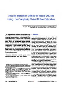
Fig. 3 Computational grid around NACA0012 airfoil
The C-type computational grid for the NACA0012 airfoil test case is shown in Fig. 3. It is a structured grid generated by the elliptic grid generator. In Fig. 4, the calculated steady pressure coefficient results for test case 1 are presented and compared with experimental data 42
o.8
'k
a
Re 4.01·106 4.09·106
...
(-----
Table 1 NACA0012 steady test cases
Ma 0.756 0.803
-05
-0.5
u'
3.1. NACA0012 results
Test case
F. Majic, Z. Virag
Viscous-Inviscid Interaction Method for Steady Transonic Flow
TRANSACTIONS OF FAMENA XXXV-2 (2011)
,,,
0.2
0.4
,,;,
Eulcr+BL Experiment lower! RANS lower Euler lower 0.8
·
I
0.8
Fig. 5 NACAOO 12 steady pressure coefficient distribution for the upper (left) and 6 the lower (right) airfoil contour for test case 2, Ma=0.803, Re=4.09 · 10 , a=0.05'
TRANSACTIONS OF F AMEN A XXXV-2 (2011)
43
F. Majic, Z. Virag
Viscous-Inviscid Interaction Method for Steady Transonic Flow
The superscripts o and n represent the old and the new solution of transpiration velocity magnitude in two successive iterations respectively. f3 represents the under-relaxation factor and its value is smaller than one. In the .near separation test cases, which are the most difficult cases for such methods, the under-relaxation factor adopts very small values around 0.001. This is the most critical part of the method. At the initial calculation step when the transpiration velocity magnitude is calculated for the first time, its old value is equal to zero. The left hand side of equation (32) is a resulting transpiration velocity magnitude and it serves as the old solution in the subsequent iteration. 3. Results and discussion The results for five steady test cases with and without the appearance of a shock wave are shown. First two test cases are calculated with the NAC0012 airfoil, the third with the NACA64AO 10 airfoil and the last two with the NLR 730 I supercritical airfoil. These airfoils show three different characteristic pressure distributions. The calculated results for the viscous-inviscid interaction method are compared with the test cases from AGARD reports [ 11 ], [12] and with the RANS code Tau [13] for the NACA0012 airfoil only. For other two airfoils, the viscous-inviscid results were compared with experimental data only. All calculations in the Tau code were performed with the two-equation k-oo based turbulence model LEA (Linearized Explicit Algebraic stress model) which is derived by Rung from the RQEVM (Realizable Quadratic Explicit Algebraic Stress Model) [14]. The flow was treated as completely turbulent without limiting the production of turbulence in the laminar part of the boundary layer.
and the RANS results for the upper (left side of the figure) and the lower (right side of the figure) airfoil contour. The calculated results show good agreement with experimental data. Two little jumps in the pressure coefficient on the upper and the lower side for the viscousinviscid results and the experimental data can be observed. The first jump is because of a weak shock wave and the second one because of the existence of transition region in the boundary layer. The transition region jump is indicated in the figure. Small deviations of RANS results compared to experimental data can be observed at the weak shock wave position, while the viscous-inviscid method gives good results in this position. Small deviations of RANS results compared to experimental data can be observed at the weak shock wave position, while the viscous-inviscid method gives good results in this position. The viscous-inviscid method shows small deviations at the trailing edge of the airfoil. It is shown that the transition method e" (where n = 9) accurately estimates the transition region of the boundary layer. From the pressure coefficient distribution it seems that the RANS results calculated with the turbulent flow for the whole region give a too strong shock wave with respect to the experimental data. The reason for -!~-------------,
In Table I the selected test cases for the NACA0012 airfoil from experimental data in the AGARD report [ 11] are presented. Two test cases at different Mach numbers, which cover the subsonic compressible flow with the occurrence of a shock wave, are selected.
u·
1
2
0.5
0.5
i 0.2
0.4
- - - Euler~BL lower • Expenment lower
Eulcr+BL upper Experiment upperl RANS upper 0.6
1
r-----· RANS lower 0.2
0.8
0.4
0.6
Fig. 4 NACAOO 12 steady pressure coefficient distribution for upper (left) and lower (right) airfoil contour for test case 1, Ma=0.756, Re=4.0l · 106 , a= -0.01°
-0.01° 0.05°
this can be in the steeper growth in displacement thickness in the turbulent boundary layer than in the laminar boundary layer. This leads to compression in the outer inviscid flow which causes the shock wave to appear at smaller angles of attack. .\,--------------, -!~-------------, -0.5
·0.5
u'
u" 05
0.5
lowe;l
I-.
·1
-0.5
- - - - -
~-·---·· I
Fig. 3 Computational grid around NACA0012 airfoil
The C-type computational grid for the NACA0012 airfoil test case is shown in Fig. 3. It is a structured grid generated by the elliptic grid generator. In Fig. 4, the calculated steady pressure coefficient results for test case 1 are presented and compared with experimental data 42
o.8
'k
a
Re 4.01·106 4.09·106
...
(-----
Table 1 NACA0012 steady test cases
Ma 0.756 0.803
-05
-0.5
u'
3.1. NACA0012 results
Test case
F. Majic, Z. Virag
Viscous-Inviscid Interaction Method for Steady Transonic Flow
TRANSACTIONS OF FAMENA XXXV-2 (2011)
,,,
0.2
0.4
,,;,
Eulcr+BL Experiment lower! RANS lower Euler lower 0.8
·
I
0.8
Fig. 5 NACAOO 12 steady pressure coefficient distribution for the upper (left) and 6 the lower (right) airfoil contour for test case 2, Ma=0.803, Re=4.09 · 10 , a=0.05'
TRANSACTIONS OF F AMEN A XXXV-2 (2011)
43
F. Majic, Z. Virag
Viscous-Inviscid Interaction Method for Steady Transonic Flow
In Fig. 5, the NACA0012 steady state calculated results and the experimental data on the upper (left side of the figure) and the lower (right side of the figure) airfoil contour are presented for test case 2. This test case represents the flow with a strong shock wave. The calculated results and experimental data show the existence of strong shock wave at the position of 45% of the airfoil chord length from the leading edge, which is in good agreement with experimental data. Viscous effects move the shock wave position toward the airfoil leading edge, which can be seen in Fig. 5 where the solution for inviscid flow (Euler solution) is also given. The results for the inviscid flow give the shock wave position moved toward the trailing edge with respect to the viscous flow solutions. This test case and similar test cases, where a strong shock wave appears, represent a difficult task for the viscous-inviscid interaction method presented in this article. This difficulty appears as a slow convergence rate and non-monotone convergence. To stabilize the convergence, under-relaxation is employed. A possible reason for instability is the boundary layer coupling by transpiration velocity and the direct solution method of boundary layer equations. Test case 2 is close to the separation bubble occurrence where the direct solution method of boundary layer equations is singular. 3.2. NACA64A010 results A test case for the NACA64A010 airfoil is selected from the AGARD report (12]. Flow conditions are presented in Table 2. Table 2 NACA64AOIO steady test case
Test case 3
Ma
Re
0.796
12.56· 10
6
a -0.21°
For the Euler solution, the structured C-type grid which consisted of 9600 control volumes was used. A close view of the grid around the NACA64A010 airfoil is shown in Fig. 6.
0
x
F. Majic, Z. Virag
Viscous-Inviscid Interaction Method for Steady Transonic Flow
of the shock wave, a lambda shaped compression shock appears. As a consequence, the shock wave intensity is smoothed and this can be seen in the pressure coefficient distribution on the airfoil contour [15], (16]. On the front part of the lower surface, the numerical solution shows a noticeable deviation from experimental data. ·1------------~
..
-0.5
·O 5
u"
u"
05
0.5
0.2
Euler+BL upper
l~-~~lcr+BL lower
Experiment upper
L-~-
·o.s
04
o.e
02
.
.J
______! __ __E_~p~nment
lower
.J
1
-0.5
-0.5
~
u·
u·
Viscous-Inviscid Interaction Method for Steady Transonic Flow
F. Majic, Z. Virag
At the trailing edge, the method shows pressure oscillations on the upper airfoil contour where the turbulent boundary layer is extremely thick. This could be explained by the separation of type B described in [ 18]. The reason for such separation lies in a steep pressure gradient towards the trailing edge and this type of separation starts from the trailing edge (rear separation). The rear separation depends strongly on the boundary layer thickness, the velocity profile of the boundary layer approaching the trailing edge, and on the pressure gradient. Therefore, the B-type separation is very sensitive to the location of the point where transition takes place. Also, the reason for pressure oscillations at the trailing edge could be in the violation of normal boundary layer assumption (aplan=O) at the trailing edge, namely the pressure gradient perpendicular to the boundary layer direction near the trailing edge can be significant. 4. Conclusion
In this study, a simple and accurate method for steady aerodynamic load prediction is developed. The steady test cases were performed for the NACA00!2, NACA64A010, and NLR7301 airfoils. The test cases for the NACA0012 and NACA64A010 airfoils were run for a transonic flow with the occurrence of a shock wave, while the NLR7301 cases were run for a subsonic flow and a transonic flow without the occurrence of shock waves. All test cases were run in the range of angles of attack where no massive flow separation is expected. The obtained results are compared with experimental data and with the calculated results of steady RANS code. The calculated steady results for the NACA0012 and NACA64A010 airfoils show good agreement with the experimental data at all Mach numbers. For these two airfoils, the position of transition is accurately predicted. In the case without shock, the transition is indicated as a small jump in the distribution of the pressure coefficient, as in the experimental data. In the cases with a shock wave, transition occurs at the shock position, so it is not clearly evident. For the two airfoils, the strength of shock wave is well predicted but its position is slightly moved toward the trailing edge with respect to the experimental data. The developed method predicts the shock wave position closer to the experimental one than the pure inviscid method, which means that accounting for the boundary layer effects improves the result accuracy. The results for the NLR7301 airfoil (which represents a challenge for viscous-inviscid methods because of extremely big nose radius) show strong sensitivity to the boundary layer thickening and the position of transition point. The developed method for this airfoil shows results with moderate agreement in pressure distribution prediction. Also, the predicted transition point on the compression side of the airfoil is not positioned in the right place and the method shows pressure instabilities at the suction side of the trailing edge. It can be concluded that the inclusion of boundary layer into the steady Euler method results in a more accurate prediction method for steady aerodynamic loads. The developed method is fast and gives results of nearly the same accuracy as a higher mathematical model like RANS and of good agreement with experimental data. REFERENCES
05
0.5
0.2
0.4
-x/c
0.6
0.8
[l]
0.2
0.4
,,,
0.6
0.8
[2]
Leifsson, L., Koziel, S.: Multi-fidelity design optimization of transonic airfoils using physics-based surrogate modelling and shape-preserving response prediction, Journal of Computational Science, Vol. 1, No. 2, 20 IO., p. 98-106 Hacioglu, A., Ozkol, I.: Transonic Airfoil Design and Optimisation by Using Vibrational Genetic Algorithm, Aircraft Engineering and Aerospace Technology, Vol. 75, No. 4, 2003.
Fig. 9 NLR7301 steady pressure coefficient distribution for test case 4 (left) and test case 5 (right)
46
TRANSACTIONS OF FAMENA XXXV-2 (2011)
TRANSACTIONS OF FAMENA XXXV-2 (2011)
47
F. Majic, Z. Virag
Viscous-Inviscid Interaction Method for Steady Transonic Flow
(3]
Anderson, W.K., Thomas, J.L., Van Leer, B.: Comparison of Finite Volume Flux Vector Splittings for the Euler Equations, AIAA Journal, Vol. 24, No. 9, 1986., 1453 - 1460
[4]
Thomas, J.L., Salas, M.D.: Far-Field Boundary Condition for Transonic Lifting Solutions to the Euler Equations, AIAA Journal, Vol. 24, No. 7, 1986., 1074-1080
[5]
Drela, M., Giles, M.B.: Viscous-Inviscid Analysis of Transonic and Low Reynolds Number Airfoils, AIAA Journal, Vol. 25, No. 10, 1987., 1347-1355
[6]
Majic, F.: Boundary Layer Method for Unsteady Aerodynamic Loads Determination, doctoral thesis, Universitiy of Zagreb, Zagreb, 2010.
[7]
Obremski, H.J., Morovkin, M.V., Landahl, M.T.: A Portfolio of Stability Characteristics of Incompressible Boundary Layer, AGARD-ograph 134, NATO, Neuilly Sur Seine, France, 1969.
[8]
Drela, M.: Two-Dimensional Transonic Aerodynamic Design and Analysis Using the Euler Equations, Ph.D. thesis, Massachusetts Institute of Technology, 1986. Lighthill, M.J.: On Displacement Thickness, Journal offluid Mechanics, Vol. 4, No. 4, 1958., 383-392
(9] [I OJ
Goldstein, S.: On Laminar Boundary-Layer Flow Near a Position of Separation, Quarterly Journal of Mechanics and Applied Mathematics, No. I, 1948., 43-69
[ 11]
Thibert, J.J., Grandjacques, M., Zwaaneveld, J.: Experimental Data Base for Computer Program Assessment - Report of the Fluid Dynamics Panel Working Group 04, AGARD-AR 138, 1979. Landon, R.H., Davis, S.S.: Compendium of Unsteady Aerodynamic Measurement, AGARD-R 702, August 1982.
[ 12] [13]
Deutsches Zentrum fiir Luft- und Raumfahrt: Technical Documentation of the DLR TAU-Code
[14]
Rung, T., Lilbcke, H., Franke, M., Xue, L., Thiele, F., Fu, S.: Assessment of Explicit Algebraic Stress Models in Transonic Flows, Engineering Turbulence Modelling and Experiments 4, Proc. 4th Int. Symposium on Engineering Turbulence Modelling and Measurements, Corsica, France, Elsevier, Amsterdam, 1999., 659-668
[15]
Magnus, R., Yoshihara, H.: Inviscid Transonic Flow Over Airfoils, AIAA Journal, Vol. 8, No.12, 1970., 2157-2161
[16]
Anderson, J.D.Jr.: Modem Compressible Flow, McGraw-Hill Publishing Company, 1990.
[ 17]
Soda, A.: Numerical Investigation of Unsteady Transonic Shock/Boundary Layer Interaction for Aeronautical Applications, Forschungsbericht 2007-03, Deutsches Zentrum filr Luft- und Raumfahrt, March 2007.
[18]
Tijdeman, H.: Investigation of the Transonic Flow Around Oscillating Airfoils, NLR TR 77090 U, October 1977.
Nagib Neimarlija Muhamed Bijedic Jure Marn
ISSN 1333-1124
THERMODYNAMIC PROPERTIES OF LIQUID METHANE, PROPANE, AND REFRIGERANT HFC-134A FROM SPEED-OF-SOUND MEASUREMENTS
UDC 536.7:546.2 Summary
The procedure of deriving thermodynamic properties of liquids from the speed of sound is recommended. It is based on the numerical integration of ordinary differential equations (ODEs) (rather than partial differential equations (PD Es)) connecting the speed of sound with other thermodynamic properties in the T-p domain. It enables more powerful methods of higher-order approximation to ODEs to be used (e.g. Runge-Kutta) and requires only the Dirichlet conditions. It was tested on the examples of liquid methane in the temperature range of 120-170 K and the pressure range of 5-50 MPa, liquid propane in the temperature range of 150-300 K and the pressure range of 5-50 MPa, and liquid refrigerant HFC-134a in the temperature range of 210-350 Kand the pressure range of 5-50 MPa. Densities of liquid methane, propane, and HFC- l 34a were derived with absolute average deviation of 0.002, 0.007, and 0.003%, respectively. Isobaric molar heat capacities of liquid methane, propane, and HFC-l 34a were derived with absolute average deviation of 0.128, 0.136, and 0.095%, respectively. lsochoric molar heat capacities of liquid methane, propane, and HFC-l 34a were derived with absolute average deviation of0.088, 0.227, and 0.057%, respectively. Keywords:
density, heat capacity, speed ofsound, finite differences, Runge-Kulla
1. Introduction
Submitted:
08.3.2011
Dr. sc. Frane MajiC Prof. dr. sc. Zdravko Virag
Accepted:
48
03.6.2011
Faculty of Mechanical Engineering and Naval Architecture, Ivana Lucica 5, 10000 Zagreb, Croatia TRANSACTIONS OF FAMENA XXXV-2 (2011)
Several articles dealing with the derivation of thermodynamic properties of liquids from experimental speeds of sound have been published in the last 40 years. An exact method of computing volume changes under high pressure from the speed of sound was developed and its application illustrated with liquid mercury at pressures up to 1300 MPa at temperatures of 295.05 K, 313.65 K, and 316.05 K [1). An iterative method of calculation was used to determine thermodynamic properties of water from the speed of sound in the pressure range of 0.1 to 350 MPa and the temperature range of 251.15 to 293.15 K [2]. The effect of pressure on the sound velocity and density of liquid toluene and n-heptane was investigated at pressures up to 260 MPa, in the temperature ranges of 173 to 320 K and 185 to 310 K [3]. Density, isothermal compressibility, isobaric thermal expansivity, and isobaric heat capacity were derived from the speeed of sound in liquid benzene and cyclohexane in the temperature range of 283 to 323 K and at pressures up to 170 and 80 MPa, respectively [4]. TRANSACTIONS OF FAMENA XXXV-2 (2011)
49