Visibility, Occlusion, and the Aspect Graph1 - CiteSeerX

Visibility, Occlusion, and the Aspect Graph1 Harry Plantinga University of Pittsburgh

Charles R. Dyer University of Wisconsin - Madison

Abstract In this paper we study the ways in which the topology of the image of a polyhedron changes with changing viewpoint. We catalog the ways that the topological appearance, or aspect, can change. This enables us to find maximal regions of viewpoints of the same aspect. We use these techniques to construct the viewpoint space partition (VSP), a partition of viewpoint space into maximal regions of constant aspect, and its dual, the aspect graph. In this paper we present tight bounds on the maximum size of the VSP and the aspect graph and give algorithms for their construction, first in the convex case and then in the general case. In particular, we give bounds on the maximum size of Θ(n2 ) and Θ (n6 ) under an orthographic projection viewing model and of Θ(n3 ) and Θ(n9 ) under a perspective viewing model. The algorithms make use of a new representation of the appearance of polyhedra from all viewpoints, called the aspect representation or asp. We believe that this representation is one of the significant contributions of this paper.

1 This work was supported in part by the NSF under grants DCR-8520870 and IRI-8802436.

Index terms: aspect graph, aspect representation, visual potential, object recognition, characteristic views, occlusion

Footnotes 1 This work was supported in part by the NSF under grants DCR-8520870 and IRI-8802436. 2 This example is due to John Canny [38].

Table of Contents 1. 2. 3. 4.

Introduction.......................................................................................................................................... 1 Visibility and Occlusion ...................................................................................................................... 3 The Viewpoint Space Partition and the Aspect Graph........................................................................ 4 Convex Polyhedra................................................................................................................................ 6 4.1. Orthographic Case .................................................................................................................. 6 4.2. Perspective Case ..................................................................................................................... 8 5. Non-Convex Polyhedra ....................................................................................................................... 8 5.1. Orthographic Case .................................................................................................................. 8 5.1.1. Occlusion under Orthographic Projection.................................................................. 8 5.1.2. An Upper Bound ........................................................................................................ 12 5.1.3. A Lower Bound .......................................................................................................... 12 5.1.4. An Algorithm ............................................................................................................. 14 5.1.4.1. The Aspect Representation ........................................................................... 14 5.1.4.1.1. Asps and Visibility ........................................................................... 17 5.1.4.1.2. Aspect Surfaces ................................................................................ 19 5.1.4.1.3. Size of Asps ...................................................................................... 22 5.1.4.1.4. Constructing the Asp ........................................................................ 23 5.1.4.2. Using the Asp to Construct the VSP ............................................................. 23 5.2. Perspective Case ..................................................................................................................... 24 5.2.1. Occlusion under Perspective Projection..................................................................... 24 5.2.2. Upper Bound .............................................................................................................. 25 5.2.3. Lower Bound.............................................................................................................. 25 5.2.4. An Algorithm ............................................................................................................. 26 5.2.4.1. The Asp under Perspective Projection .......................................................... 26 5.2.4.2. Using the Asp to Construct the VSP ............................................................. 27 6. Conclusion ........................................................................................................................................... 28 References................................................................................................................................................. 29

1. Introduction A number of researchers in computer vision have suggested that a reasonable approach to 3-D object recognition is the “characteristic view” approach, in which several characteristic 2-D views of an object are stored and all are compared to an image for recognition [1-6]. The idea behind this approach is that if a stored view is similar to the image, the recognition process will be simple and fast. The approach works well in parallel, since the image can be compared with characteristic views in parallel. The views are generally taken to be topologically distinct in the interest of minimizing the number of views that must be stored, with the idea that a topological match of the image and the view should be sufficient for recognition. In order to calculate these characteristic views one must calculate regions of viewpoints with particular appearance characteristics, such as regions of viewpoints in which the object has the same “topological appearance.” Computing viewpoints with particular appearance characteristics is important in other problems as well. In the automatic visual inspection of parts, a computer may control a mobile camera in order to inspect a part and determine whether it was manufactured correctly. In order to do so, the computer must be able to direct the camera to a viewpoint from which it can see appropriate sections of the part. In motion planning, visibility and free-space computations are basic to finding collision-free paths. In this paper we show how to find and represent regions of viewpoint space of particular visibility characteristics and boundaries in viewpoint space at which the appearance changes. We do this by cataloging the ways that the topological appearance, or aspect, of a polyhedron can change with changing viewpoint. These changes we call events. The events give rise to boundaries in viewpoint space, separating regions of viewpoints from which the aspect is different. Finding all of these boundaries enables us to construct a partition of viewpoint space into regions of constant aspect, which we call the viewpoint space partition (VSP). One use of the VSP is to construct the aspect graph, a graph with a vertex for every aspect and edges connecting adjacent aspects. We will show how to do this under two viewing models. The first uses orthographic projection and restricts viewpoints to directions corresponding to points on a unit sphere, and the second uses perspective projection and allows viewpoints anywhere in the world. We give tight bounds on the maximum sizes of the VSP and the aspect graph in all cases, thus determining the maximum number of topologically-distinct views of an object. In Table 1 we present a summary of the size of the VSP and aspect graph in various cases, and in Table 2 we present a summary of the time required to construct them under various conditions by the algorithms given here. convex polyhedra

non-convex polyhedra

orthographic

O(n2)

O(n6)

perspective

O(n3)

O(n9)

Table 1. The maximum size of the VSP and aspect graph.

convex polyhedra

non-convex polyhedra

orthographic

O(n2)

O(n6 log n)

perspective

O(n3)

O(n9 log n)

Table 2. Construction time for the VSP and aspect graph.

Koenderink and van Doorn [7] laid the groundwork for the study of the topologically-distinct views of an object in their analysis of the singularities of the visual mapping for a smooth body. The singularities of the visual mapping are points of the image that map to points in the world at local minima and maxima of distance and points on surfaces tangent to the viewing direction. They catalog the ways that the topological structure of the singularities can change and show that for most vantage points the structure of the singularities does not change with small changes in viewpoint. They call a change in the

1

topological structure an “event,” and they catalog the different kinds of events that occur for smooth bodies. In a later paper [8], Koenderink and van Doorn define an “aspect” as the structure of the singularities of a stable view of a smooth object, and they define the “visual potential” graph for such an object, which we call the aspect graph. They are concerned primarily with smooth bodies, but they also discuss smooth approximations to polyhedra. Some previous work has been published on constructing the aspect graph. Gualtieri et al. [9] show how to construct an aspect graph for a convex polygon with viewpoint constrained to lie in the plane containing the polygon, using perspective projection. Watts [13] describes an O(n4)-time algorithm for enumerating the “principal views” (similar to aspects) of a convex polyhedron under perspective projection. McKenna and Seidel [10] construct minimal and maximal shadows of convex polyhedra in a plane. In doing so, they project the great circles corresponding to the faces onto a plane and construct the resulting arrangement of the lines in the plane using the O(n2 ) algorithm of McKenna and Seidel [10] or Edelsbrunner et al. [11]. The result is similar to the VSP for convex polyhedra under orthographic projection. Kender and Freudenstein [12] discuss the meanings of terms such as “degenerate view,” “characteristic view,” “visual event,” and “general viewing position.” More recently, Plantinga and Dyer [14, 15] show how to construct the aspect graph for convex and non-convex polyhedra under orthographic projection. Gigus and Malik concurrently developed an algorithm for the same problem, with the same worst-case run-time of O(n6 log n) [16], but their algorithm appears to require much more time for problem instances that are not worst-case. Gigus, Canny, and Seidel give an improved version of the previous algorithm [17], with better average-case behavior. Stewman and Bowyer [18] and Bowyer, et al. [1] give an algorithm for constructing the aspect graph for non-convex polyhedra, without analysis of time complexity. They also discuss constructing the aspect graph for right, circular, straight, homogeneous generalized cylinders. Rosenfeld [5] suggests that fast object recognition will require representing an object as a series of 2-D “characteristic views” or “aspects.” Various approaches have been taken in selecting an appropriate set of views for an object. Views may be selected on the basis of how likely they are to occur in an image. For example, a view of an object in a stable, upright position of constant aspect over a wide range of viewing directions is more likely to occur than many other views. Researchers have used different numbers of characteristic views, ranging from a small or moderate constant (up to about 300) [3, 4, 19-21] to every topologically distinct view of the object, i.e. a view for every vertex in the aspect graph [1, 2, 22]. Schneier et al. propose that the aspect graph be used as part of a general representation for computer vision [6]. Several approaches to object recognition make use of a fixed set of views of an object from regularly-spaced viewpoints and then construct a hierarchy or tree of visual features [23-29]. Related problems in the general area of visibility have also received attention. In computer graphics much work has been done on hidden-line removal (see, for example, Sutherland et al. [30]), which is essentially computing the visibility of a scene from a particular viewpoint. El Gindy and Avis [31] and Lee [32] compute the “visibility polygon” from a point in the plane, that is, the list of edges visible from the point. Avis and Toussaint [33] compute the visibility of a polygon in the plane from some viewpoints along an edge in the plane. Canny [34] computes the region of a plane of viewpoints from which a polygon in R3 is visible and gives an algorithm for constructing the “shadow” of a polygon relative to another polygon on the plane of viewpoints. Other work has also been done on the visibility polygon from an edge [35-37]. The major contributions of this paper are tight bounds on the maximum size of the VSP and the aspect graph in various cases, efficient algorithms for their construction, and the introduction of the aspect representation. Upper bounds on problems equivalent to the orthographic case have appeared earlier [10, 11], and the lower bound on the orthographic case is due to Canny [38], but bounds on the non-convex perspective case have not appeared elsewhere. The algorithms given for constructing the VSP and aspect graph for convex polyhedra are optimal for all but highly degenerate polyhedra. The algorithms given for non-convex polyhedra are efficient in the sense that the time required is O(log n) larger than the output size for all but highly degenerate polyhedra. The algorithms of Gigus and Malik [16] and Gigus et al. [17] for the orthographic case, developed concurrently with this work, have the same worst-case performance, but no claim is made about performance in terms of output size in either case. The runtime of the algorithm of Bowyer, et al. [1] for the perspective case has not been analyzed. The asp, used in

2

construction of the VSP, is interesting in its own right; it has already proved useful for other problems [15, 39, 40]. Section 2 introduces the notions of visibility and occlusion and describes the viewing models used in this paper. Section 3 defines the viewpoint space partition and the aspect graph and discusses some of their properties. Section 4 contains proofs of upper and lower bounds on the maximum size of the VSP and the aspect graph for convex polyhedra and presents an algorithm for their construction. These are done under both the orthographic and the perspective viewing models. Section 5 considers the same problems for the case of non-convex polyhedra. The types of boundaries of changing aspect that occur for non-convex polyhedra are characterized, and upper and lower bounds on the maximum size of the VSP and the aspect graph and algorithms for their construction are presented, under the orthographic and perspective viewing models. Section 6 contains concluding remarks. 2. Visibility and Occlusion In this paper we assume that the world contains solid, opaque polyhedra and that the edges of the polyhedra are visible in the image, i.e., are projected into the (unbounded) image plane using orthographic or perspective projection. We assume that the resolution of the image is infinite; nothing is too small to resolve. Note that under these models the image of a polyhedron is a line drawing of the appearance of the polyhedron with hidden lines removed. We will also speak of a viewing direction, the direction in which the camera or viewer is pointed. We assume that the camera has a fixed orientation with respect to the viewing direction. The directions of incident ambient light represented in the image plane are those greater than 90° away from the viewing direction (since the viewing direction is away from the viewer but the visible light is toward the viewer). In problems such as motion planning, visibility information from all directions is of interest, since the visible surfaces represent the boundaries of free space in any direction. Visibility from all directions can be represented by two image planes from opposite viewing directions along with points at infinity in one of the planes or by an image sphere representing all viewing directions. For the problem of looking at an object and recognizing it or perceiving its shape, however, a section of a single image plane is sufficient. In the perspective model, we represent a viewpoint as a point in 3-space; the viewing direction is the ray from the viewpoint to the origin of the world coordinate system. In the orthographic model, we need only represent the viewing direction. We represent these directions as points on a unit sphere, with a point representing the direction from that point to the origin. We will speak of points on the unit sphere and viewing directions interchangeably. We will denote viewing directions by (θ,φ) (see Figure 1).

3

y

φ

x

θ z Figure 1. The point ( θ,φ) on the unit sphere denoting a viewing direction with respect to the origin of the world coordinate system (x,y,z).

Thus, a reference direction (0,0,1) rotated by θ counterclockwise about the y-axis and then by φ counterclockwise about the x-axis corresponds to the viewing direction (θ,φ). (In Figure 1, we show a negative φ and positive θ rotation). The orientation of the image plane with respect to the line of sight is assumed fixed. The orientation of the image plane when φ = ±90° is defined to be the orientation as φ approaches 90° while θ = 0°. In this paper we characterize the way that the structure of the image changes with changing viewpoint by studying the viewpoints at which such changes occur. These viewpoints are on the boundaries in viewpoint space of volumes of viewpoints from which the world has the same topological appearance, i.e. the structure of line segments and intersection points in the image is the same. Note that events do not require the appearance or disappearance of regions in the image; the change may be only in the number of edges of a region (see Figure 2).

Figure 2. An event may consist only of a change in the number of sides of a polygon.

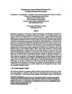
3. The Viewpoint Space Partition and the Aspect Graph We define a maximal viewing region of constant aspect, or viewing region for short, as a set of viewpoints that are equivalent under the following equivalence relation: two viewpoints v1 and v2 are equivalent whenever there is a path of viewpoints from v1 to v 2 such that from every viewpoint along the path (including v1 and v2 ) the aspect is constant, i.e. the image has the same topological structure. The equivalence classes are regions or volumes of constant aspect, i.e. viewing regions. We call this partition of viewpoint space the viewpoint space partition or VSP. In the orthographic case it consists of a partition of the sphere, and in the perspective case a partition of R3 . The boundary points of the VSP are points from which an arbitrarily small change in viewpoint causes a change in the topology of the image. Figure 3 shows a tetrahedron and Figure 4 shows the structure of the viewpoint space partition generated by the tetrahedron under orthographic projection. The viewpoint

4

space partition is flattened out onto a plane, and the topological structure but not the shape of the regions is preserved.

C

A B D

Figure 3. A tetrahedron.

ABD

D

AD

A

AB

ADC

AC

ABC

CD

C

BC

B

BD

BCD

Figure 4. The viewpoint space partition for a tetrahedron.

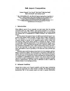
In Figure 4, each region is labelled by the faces visible from viewing directions in that region, but these labels are not a part of the definition of the VSP. Since a face is not considered to be visible edge-on, the boundary of the region in which a face is visible belongs to the complement of that region. In Figure 4, the shaded side of a boundary represents the inside of a region. We define the dual of the region-boundary structure of the VSP to be the aspect graph. That is, for every region of the VSP there is a vertex in the aspect graph, and vertices of the aspect graph are connected by edges whenever the corresponding regions of the VSP are adjacent. Thus, the aspect graph has a vertex for every aspect, and vertices for adjacent aspects are connected. Figure 5 shows the aspect graph for the tetrahedron of Figure 3.

5

BD AD

ABD

A

ACD

AB

AC

CD

C

ABC

B

D

BC

BCD

Figure 5. The aspect graph for a tetrahedron.

Note also that under our definition of the VSP and the aspect graph, two different vertices of the aspect graph can correspond to aspects that are topologically equal. This happens when the appearance of the object is the same from two different, unconnected, maximal regions of viewpoint space. Furthermore, the appearance from the two aspects can be the same in two different senses. In the more restrictive sense, the same set of faces may be visible and have the same topology from a different region of viewpoint space. In the less restrictive sense, a completely different set of faces may have the same topological appearance. These are also reasonable notions of the identity of aspects, but they differ from ours. The most appropriate notion of visibility depends on the problem. Since the aspect graph has a vertex for every topologically-distinct view of a polyhedron, it has been used for characterizing the distinct views of an object. However, the VSP represents essentially the same information with the addition of the actual boundaries in viewpoint space of the viewing regions, and the space it requires is only a constant factor larger. Thus it may be a more appropriate tool for applications that are concerned with the particular viewpoints associated with each aspect. 4. Convex Polyhedra In this section we consider the VSP and aspect graph for a single convex polyhedron. The restriction to convex polyhedra simplifies the problem because a face is always visible from viewpoints in front of it; no face ever occludes another face. The only way that a face may become invisible with changing viewpoint is by “turning away from” the viewer or “going below the horizon.” Also, in the convex case, there cannot be two vertices in the aspect graph for the same set of faces: if the same set of faces is visible from two viewpoints, that set is also visible from all viewpoints along the shortest path (geodesic) in viewpoint space connecting them. In the case of the orthographic viewing model, tight upper and lower bounds of Θ(n2 ) are shown on the maximum size of the aspect graph and VSP. In the perspective case, bounds of Θ(n3) are shown. 4.1. Orthographic Case A face of a convex polyhedron is visible in any viewing direction “pointing toward” the front of that face. That is, if d is a viewing direction and n is the outward normal of the face, that face is visible whenever n ⋅ d < 0. Therefore the boundary between the regions of the sphere of viewing directions in which the face is visible and in which it is invisible is the great circle defined by {d : n ⋅ d = 0}. This is the intersection of the sphere with a plane containing the origin and having normal n. For a convex polyhedron with n faces, the corresponding n great circles therefore partition viewpoint space into a subdivision in which the same set of faces is visible from all of the viewpoints in each region, i.e. the VSP. A pair of great circles coincides or intersects in two points, so discounting

6

coincident pairs, the n great circles have at most n (n – 1) = O(n2 ) intersection points. Thus, by planarity, the size of the VSP is O(n2). The aspect graph is the dual of the VSP, so it also has size O(n2 ). The lower bound on the maximum size of the VSP and the aspect graph for a convex polyhedron of size n under orthographic projection is Ω(n2 ). We prove this by exhibiting a class of such polyhedra. Consider a band of m square faces arranged around a circle. In Figure 6 we show two such bands arranged orthogonally around a sphere, with additional faces added to form a convex polyhedron.

Figure 6. A convex polyhedron with two orthogonal bands.

Suppose that one of the faces visible in Figure 6 is selected from each band, excluding the face that is common to both bands. The great circles bounding the visibility regions on the sphere of the two selected faces have two intersection points, and these points are vertices of the VSP. Each pair of faces thus selected has a unique pair of intersection points, so there are Ω(m2 ) vertices in the VSP. The faces and the bands form a polyhedron of size O(m), so if the polyhedron has size n, its VSP has size Ω(n 2 ). Thus the aspect graph, which is the dual of the VSP, also has size Ω(n2). In fact, a polyhedron would have to be highly degenerate to have a VSP of size less than Θ(n2). For example, any class of polyhedra with bounded vertex degree and bounded face degree has a VSP of size Ω(n2). This is because the only way to for the VSP to be smaller is for the intersection points of the great circles coincide, and if the number of edges around each face and the number of faces around each vertex is bounded, then the number of great circles that can intersect in a single point is bounded. An example of a highly degenerate class of polyhedra is the class of n-sided approximations to a cylinder; for polyhedra in this class the VSP has size O(n). The VSP is constructed by merging the great circles corresponding to the faces of the polyhedron into one subdivision data structure. This data structure represents regions, edges, and vertices of the subdivision and adjacencies of the various items. Edelsbrunner et al. [11] present an algorithm for constructing an arrangement (subdivision) formed by n lines in the plane in O(n2) time. The algorithm for constructing arrangements can be used for constructing a subdivision formed by great circles on the sphere by projecting the great circles onto two parallel planes. The projections are lines, and the arrangements of these lines are constructed in the planes. This approach is similar to that of McKenna and Seidel [10], in which they construct minimal or maximal shadows of a convex polytope generated by a point light source at infinity. Since the aspect graph is the dual of the VSP, it can be constructed by copying the region-edge subgraph of the VSP, changing the regions to vertices, and changing the edges separating regions to edges connecting adjacent vertices. This can be done in linear time in the size of the VSP, so the aspect graph can be constructed in O(n2) time. 4.2. Perspective Case Under the perspective model the image changes as the viewpoint moves in any one of three independent directions rather than two. As in the orthographic case, the only kind of occlusion that

7

occurs is when the viewpoint moves below the plane containing a face. Therefore R3 is subdivided by n planes for a polyhedron with n faces, and the resulting subdivision is the VSP. The subdivision formed in each plane by the intersections with the n – 1 other planes has O(n2 ) vertices, edges, and regions. Thus among all n planes there are at most O(n3) vertices, edges, and 2-faces of the subdivision of R3 , and therefore also O(n3) cells. Thus the VSP and the aspect graph have size O(n3) in the perspective case. The lower bound example of the orthographic case (see Figure 6) is also a lower bound in the perspective case. Consider the faces of the two bands in any octant. Any three faces from these bandquarters (two from one band and one from the other) determine a distinct vertex in the VSP since they have a distinct intersection point. There are Ω(n) faces in each quarter band, so the VSP has Ω(n3 ) vertices. The VSP must also have Ω(n3 ) cells, so the aspect graph also has size Ω(n3). As in the orthographic case, a class of polyhedra would have to be highly degenerate to have size less than Θ(n3 ). In fact, any class of convex polyhedra with bounded vertex degree and face degree has a VSP of size Ω(n3). The algorithm for constructing the aspect graph in this case is similar to that of the orthographic case. In order to construct the VSP, we find all of the intersections of the planes corresponding to the faces of the polyhedra and construct the VSP by finding its cells, faces, edges, and vertices and linking incident faces. The algorithm of Edelsbrunner et al. [11] for constructing arrangements of hyperplanes does the job in optimal, O(n3) time. The aspect graph is the dual of the cell-face structure of the VSP. It is constructed from the VSP by changing cells to vertices and faces between cells to edges joining the vertices, and deleting everything else. This algorithm requires linear time in the size of the VSP, so the aspect graph can be constructed in O(n3) time. 5. Non-Convex Polyhedra In the convex case, the only sort of event that can change the aspect is the horizon effect. In the non-convex case, faces can occlude other faces, causing several other types of events. Thus, in order to construct the VSP and the aspect graph in the non-convex case we must characterize all the ways in which aspect can change. In the following sections we list the kinds of events that can occur and the corresponding boundaries of regions of constant aspect that result in viewpoint space. 5.1. Orthographic Case In the orthographic case, the VSP is a subdivision of the sphere of viewpoints, and boundaries of regions of constant aspect are 1-D curves on the sphere. We first list the ways that the aspect can change in the orthographic case and the kinds of boundaries in viewpoint space that these changes generate. We then present upper and lower bounds on the maximum size of the VSP and aspect graph in this case and present algorithms for their construction. 5.1.1. Occlusion under Orthographic Projection In order to compute the regions of constant aspect in viewpoint space, we compute the boundaries of these regions. In order for a viewpoint to be a boundary viewpoint, there must be a configuration in the image that will change with an arbitrarily small change in viewpoint. This can happen in one of several ways, requiring essentially that some configuration of lines appears to intersect at a point in the image from a one-dimensional path of viewpoints. In this section we characterize the ways that this can occur for polyhedra. The types of boundaries are horizon boundaries, edge-vertex boundaries, and edge-edgeedge boundaries. Horizon boundaries have already been discussed; we now consider edge-vertex and edge-edge-edge boundaries. Suppose that a given viewpoint is an event and that no non-adjacent vertex-edge pair appears to intersect. The change in the image must occur at an image vertex since an arbitrarily small change in viewpoint suffices to change the image. Image vertices result from object vertices or T-junctions, and if a T-junction is the apparent intersection of only two object edges, the image doesn't change. Thus at least three object edges must appear to intersect at some image point, possibly as the apparent intersection of an object vertex and a non-adjacent object vertex.

8

Now suppose that an object vertex and non-adjacent edge appear to intersect from a given viewpoint. Changing the viewpoint slightly in some direction will separate the edge and the vertex, resulting in one of the following cases. If the vertex is in front of the edge from the given viewpoint, one of the events shown in Figure 7 occurs. If the vertex is behind the edge from the given viewpoint, one of the events shown in Figure 8 occurs. We call this type of event an edge-vertex event. Thus the viewpoints from which an object edge and an unconnected object vertex appear to intersect are boundary viewpoints.

(1)

(2)

(3)

(4)

(5)

Figure 7. Edge-vertex events with the vertex in front of the edge. In each row, the center figure shows the image from a viewpoint on the event boundary, and the left and right figures show the appearance on either side. The edges of interest are marked in bold.

(1)

(2)

(3)

(4)

(5)

Figure 8. Edge-vertex events with the vertex behind the edge. In each row, the center figure shows the image from a viewpoint on the event boundary, and the left and right figures show the appearance on either side.

9

Boundaries in viewpoint space of occlusion of this type occur at viewpoints such that a vertex of one face is directly behind an edge of another face in the image. Therefore the only candidate viewpoints for such boundaries are viewing directions parallel to the plane containing the point and the edge. That is, for a point p and an edge from p1 to p2, the candidate viewpoints are the points on the arc of the great circle with the normal (p1 – p) × (p2 – p1 ). The boundaries of the arc are the points of intersection with the lines (p,p1 ) and (p,p2 ). Since there are O(n) vertices and O(n) edges in a polyhedron or polyhedral scene, there are O(n2 ) edge-vertex pairs, so this type of occlusion is responsible for generating at most O(n2) occlusion boundaries (which are arcs of great circles) on the sphere of viewpoints. Events can also arise from the apparent intersection of three object edges in such a way that no pair of the edges meets at a vertex. Suppose that three object edges appear to intersect in a point. Let the first and second be arbitrary. Depending on the location and orientation of the third, one of the events shown in Figure 9 occurs. We call this type of event an edge-edge-edge event. If more edges or vertices meet at a viewpoint, the event can be treated as two more events from infinitesimally different viewpoints.

(1)

(2)

(3)

Figure 9. Edge-edge-edge events. In each row, the center figure shows the image from a viewpoint on the event boundary, and the left and right figures show the appearance on either side.

The boundaries in viewpoint space generated by edge-edge-edge occlusion occur at viewpoints where three unconnected edges appear to intersect in a single point. In order to find the viewing directions in which three edges appear to intersect in a point, let the endpoints of the three edges be p11, p12, p21, p22, p31, and p32 respectively, and pick a point on one of the edges, say p = p11+ t (p 12–p11), 0 ≤ t ≤ 1

(1)

The other two edges appear to intersect in some viewing direction d at p whenever the planes defined by p and each of the other two edges intersect in a line with direction d. That is, the other two edges appear to intersect at p from a viewing direction given by the intersection of the planes defined by p, p21, p22, and p, p31, p32. Normals to these planes are given by (p–p21) × (p21–p22) (p–p31) × (p31–p32) and the intersection of these two planes has the direction

10

d = [(p–p21) × (p21–p22)] × [(p–p31) × (p31–p32)]

(2)

Therefore d is a viewing direction in which the three edges appear to intersect at p. Note that d is a quadratic function of the parameter t. Thus viewing directions do not form an arc of a great circle in viewpoint space. In Eq. (2) d is given in Cartesian coordinates. In order to transform it to the ( θ,φ) notation, we can use a Cartesian-to-spherical coordinate transformation:

θ = tan–1 (dx /d z)

(3)

φ = –sin–1 (dy /√ (dx 2 + dy2 + dz2 )) 

(4)

There are O(n3 ) sets of three edges in a polyhedron, so there are O(n3) such curves in viewpoint space. Note that horizon and vertex-edge occlusion boundaries can be considered a special case of edgeedge-edge occlusion. When two of the edges of edge-edge-edge occlusion meet at a vertex of the object, the result is vertex-edge occlusion. When all three of the edges lie on the same face of the object, the result is that the viewing direction lies in the plane containing the face. In that case the viewing direction is on the boundary of occlusion caused by the face turning away from the viewer. The figures above represent an exhaustive list of the basic types of edge-vertex and edge-edgeedge events: all of the distinct (with respect to symmetry) ways that an object edge and vertex or three edges can appear to intersect have been shown. If the image changes at a point, at least one of these events must occur. Of course, more than three edges may appear to intersect at a point in the image, and several object faces or edges may then appear or disappear with a small change in viewpoint. For example, from some viewpoints almost all of the edges on the top of an n-sided approximation to a cylinder may disappear with a small change in viewpoint. Such cases may be treated as several events occurring at the same viewpoint. 5.1.2. An Upper Bound We have seen that the boundary points of occlusion are viewing directions where three object edges appear to intersect in a single point and that there are O(n3) curves of such points. O(n3 ) quadratic curves on the sphere intersect in O(n6) points. The resulting subdivision of viewpoint space is planar, so it also has O(n6 ) edges and regions. Therefore the VSP and the aspect graph both have maximum size O(n6). 5.1.3. A Lower Bound We have argued that there are O(n3) curves in viewpoint space potentially bounding regions of visibility and that there are O(n6 ) intersection points of these curves, so the VSP has size O(n6 ). In fact, these bounds are tight. We show this by presenting an example family of polyhedra with n faces that has an aspect graph (and hence a VSP) of size Ω(n6).1 Consider two grids of m strips each, with the strips close together. In front of these grids are two screens, each with m – 1 slits. The two screens and grids are arranged as in Figure 10. Note that the grid edges are not quite parallel to the screen edges.

1 This example due to John Canny [1987].

11

Figure 10. Two grids behind two screens.

In a typical view of the grids behind the screens, parts of the grids are visible through only one slit of each screen. Furthermore, only a small part of the grid is visible through the slit (see Figure 11).

Figure 11. A typical view of the two grids (seen simultaneously). This scene has an aspect graph of size Θ(n6)

The part of each grid that is visible behind the vertical screen is a portion of a nearly-vertical grid element and between 0 and m nearly-horizontal grid elements. The view through a slit of the horizontal grid is symmetrical. Figure 12 contains close-up views of the part of the grids visible through the two slits.

12

Figure 12. Close-up views through the slits.

Note that changing the viewing direction along the horizontal arrow causes the m nearly horizontal faces to disappear from view in the vertical slit and reappear one by one, generating a new boundary of occlusion in viewpoint space each time. This disappearing and reappearing of the horizontal faces in back occurs m times, so that the view through this slit requires Ω(m2 ) vertices in the aspect graph. There are Ω(m) vertical slits, requiring Ω(m2 ) boundaries each, for a total of Ω(m3 ) boundaries. Note also that the view through a vertical slit doesn't change when the viewing direction is changed parallel to the vertical arrow. These boundaries are parallel straight lines (arcs of great circles) in viewpoint space. The views through the horizontal slits exhibit the same behavior: they cause Ω(m3 ) straight boundaries in viewpoint space. However, the boundaries are orthogonal to the other Ω(m3 ) boundaries, so there are Ω(m6) intersection points of these boundaries. Therefore the VSP and the aspect graph have size Ω(m6 ). 5.1.4. An Algorithm In the convex case, the VSP is the partition of the sphere generated by the great circles corresponding to the faces of the polyhedron, but in the non-convex case, edge-vertex and edge-edgeedge events also affect the VSP. As a naive approach to constructing the VSP in this case, one might consider finding every boundary in viewpoint space that might potentially generate an event, i.e. every boundary of the form of Eqs. (3) and (4) above, taking all sets of three edges in every possible order. All O(n3 ) of these boundaries can be drawn on the sphere and the resulting subdivision constructed; the subdivision would have size O(n6 ). This subdivision is the same as that constructed by Ke and O'Rourke in the context of deriving bounds on the complexity of motion planning for a ladder [41]. However, not all of the boundaries thus constructed actually represent changes in visibility because what would otherwise be an event may be occluded from some viewpoints. Thus, to construct the VSP it remains to remove the boundaries that are not actual aspect boundaries. Since the edges that gave rise to each of the boundaries are known, the image point at which the event should occur can be computed. Thus, by computing the faces visible immediately around the image point in question from viewpoints immediately adjacent to the boundary one can determine whether the aspect actually changes at that boundary: the sets of visible faces on either side of the boundary are equal whenever the aspect does not change. Adjacent regions are merged if the same set of faces is visible from both regions. The result is the VSP, and its dual is the aspect graph.

13

This algorithm can be executed in O(n7) time, while the worst case size of the aspect graph is Unfortunately, the best-case runtime of this algorithm is also Ω(n 7 ). Even the VSP for a convex polyhedron, which has size O(n2 ), would take time Ω(n7) to construct by this algorithm. An algorithm with better behavior for simple polyhedra would be much preferable. The size of the subdivision generated by m curves is O(m2 ), so in order to construct the aspect graph more efficiently we compute the actual event boundaries before generating the subdivision. Then if the actual number of event boundaries is smaller than Θ(n3), the runtime of the algorithm will be much less than Θ(n6 log n). In order to do that, we introduce and use the aspect representation or asp for the object. The asp is defined in the next section. O(n6).

5.1.4.1. The Aspect Representation The asp is a continuous, viewer-centered representation for polyhedra: viewer centered in the sense that it represents the appearance of a polyhedron to a viewer, rather than the volume of space that it fills, and continuous in the sense that it represents appearance as a continuous function of viewpoint rather than from a discrete set of viewpoints. Since the asp represents all of the visual events related to the viewing of the polyhedron, it is a straightforward procedure to calculate the aspect boundaries in viewpoint space from the asp. We first define aspect space, which is intended to be a space in which to represent the appearance of an object from all viewpoints. In the orthographic case, it is the tangent bundle of planes on the sphere, representing an image plane for every viewpoint. If we denote a viewpoint by (θ,φ) and a point in the image plane by (u,v), then we can denote a point of aspect space by (θ,φ,u,v). We then define the volume of aspect space occupied by the appearance of a point, edge, or polygon to be the set of points of aspect space occupied by the appearance of the object. That is, the point (θ,φ,u,v) is in the volume of aspect space for the appearance of the object whenever (u,v) is in the image of the object from the viewpoint ( θ,φ). We will use a boundary representation for such a volume of aspect space, and we will call it the aspect representation or asp for the point, edge, or polygon. The asp includes a representation of all of the surfaces bounding the corresponding volume of aspect space and pointers from surfaces to incident surfaces that have dimension one degree higher or lower. Thus, the asp for a polygon includes a representation of the 3-surfaces in this 4-D space bounding the volume, the 2-surfaces bounding each 3-surface, and so on, together with pointers between incident surfaces. The forms of the bounding surfaces are derived below, and in the asp they are represented as a set of constants (and implicitly the set of equations for that type of surface). Note that the (θ,φ) cross-section of the asp for the polygon is the appearance of the polygon from the viewpoint (θ,φ), with edges of the polygon represented by the cross-section of asp 3surfaces. Given a point (x0,y0,z0) in a fixed coordinate system, we can calculate the points in aspect space occupied by its appearance by considering what happens to the image of the point as the viewpoint changes. The projection onto the image plane can be separated into two parts, a rotation so that the viewing direction is along the z-axis and an orthographic projection into the z=0 plane. The rotation is given by

 cos θ 0 sin θ 1 0 [x0 ,y0,z 0 ]  0  –sinθ 0 cos θ 

0  1 0    0 cos φ –sin φ  =   0 sin φ cos φ   

[x0 cos θ – z0 sin θ, x0 sin θ sin φ + y0 cos φ + z0 cos θ sin φ, x0 sin θ cos φ – y0 sin φ + z 0 cos θ cos φ] After orthographic projection into the image plane (u,v), this yields

14

(5)

u = x0 cos θ – z0 sin θ

(6)

v = x0 sin θ sin φ + y0 cos φ + z0 cos θ sin φ

(7)

The points (θ,φ,u,v) defined by the above equations represent the volume of aspect space occupied by the appearance of the points. Notice that the equations have two degrees of freedom, θ and φ. Thus the appearance of a point in 3-space occupies a 2-surface in aspect space. The asp for this volume is an unbounded 2-D surface, represented by the constants x0, y0, and z0 and Eqs. (6) and (7) above. The appearance of a line segment occupies a 3-surface in aspect space bounded by 2-surfaces. It can be written down directly by substituting parametric equations for a line segment into the point equations. We use a parametric representation for the line segment from (x 0,y0,z0) to (x1,y1,z1), with parameter s varying from 0 to 1. Letting a1 = x1–x0, b1 = y1–y0, and c1 = z1–z0 we have x(s) = x1 + a1 s y(s) = y1 + b1 s z(s) = z1 + c1 s

(8)

The point equations become u = (x1 + a1 s) cos θ – (z1 + c1 s) sin θ

(9)

v = (x1 + a 1 s) sin θ sin φ + (y1 + b1 s) cos φ + (z1 + c1 s) cos θ sin φ

(10)

These functions define a 3-surface in aspect space if θ, φ, and s are variables. The bounding 2-surfaces are given by Eqs. (6) and (7) above for the points (x0,y0,z0) and (x1,y1,z1). Thus the asp for a line segment includes a representation of the 3-surface and pointers to the bounding 2-surfaces. Given a polygon in object space, there is a bounding 3-face in the asp corresponding to each edge of the polygon. The 3-surfaces are represented with the constants of Eqs. (9) and (10) above, together with pointers to the incident 2-surfaces. Each 2-surface corresponds to a vertex of the polygon and is represented by the constants in Eqs. (6) and (7), which also happen to be the coordinates of the vertex in object space. Figure 13 shows the asp for an example polygon, the triangle (1,1,0), (2,1,0), (1,2,0) in object space. Since it is difficult to represent a 4-D volume in a 2-D figure, the figure shows two 3-D cross-sections of the asp at different fixed values of φ. The 2-D cross-sections of the asp within each 3-D cross-section are the images of the triangle for the corresponding values of θ and φ. The asp represents all of these cross-sections continuously by representing the bounding surfaces. y

x z

Figure 13a. The triangle (1,1,0), (2,1,0), (1,2,0) in object space.

15

v

v

u

u

θ

θ Figure 13b. A cross-section of the asp for the triangle for φ = 0˚.

v

v

u

θ

u

θ Figure 13c. A cross-section of the asp for the triangle for φ = 30˚.

In general, the surfaces bounding asps are not planar, so an asp is not a polytope (i.e. the generalization of a polygon, polyhedron, etc.). However, the surfaces are well-behaved: the trigonometric functions in the equations for the surfaces can be eliminated by a spherical-to-Cartesian coordinate transformation of the representation for viewpoints, from ( θ,φ) to V = (vx , vy , vz). As a result, the surfaces are algebraic, and each can be represented with a few constants. Therefore we can work with the surfaces in much the same manner as we would work with lines and planes in a polyhedron. For example, we can calculate the intersection of any two of these surfaces in closed form. The intersection of two 3-surfaces is a 2-surface and, with the viewpoint transformation above, it is a linear function of viewpoint. This kind of surface occurs in edge-vertex occlusion (Section 5.1.1.1). The intersection of three 3-surfaces is a 1surface, a quadratic function of viewpoint. This kind of surface occurs in edge-edge-edge occlusion (Section 5.1.1.2). A vertex is the result of the intersection of four 3-surfaces; it is a cubic function of viewpoint. The equations for these surfaces are developed below. Thus, while the asp is not a polytope, we speak of it as if it were. Specifically, we refer to the 3surfaces that bound an asp as facets, the 2-surfaces that bound the facets as ridges, and the 1-surfaces or curves as edges. A 4-D volume of aspect space bounded by facets is referred to as a cell. We will refer to a partition of a region of aspect space into cells as a subdivision. We can also work with asps much as we would with polyhedra. For example, we can determine whether two asps intersect by determining whether some face of one intersects some face of the other, and if not, whether one is completely inside the other.

16

5.1.4.1.1. Asps and Visibility Consider the asp for a point. Eqs. (6) and (7) for the asp for that point are defined for all values of θ and φ. This is as one would expect, since a point is visible from any viewing direction. We can represent a point which is not visible from every viewing direction, say a point which is occluded in some directions by a polygon, by putting bounds on the values of θ and φ for Eqs. (6) and (7) above. That is, if we represent only a part of the surface for the point in aspect space, rather than the whole surface, we have the asp for a point which is visible from only some viewpoints. In fact, a fundamental property of aspect space is that occlusion in object space corresponds to set subtraction in aspect space. That is, if one polygon partially occludes another, we can characterize the appearance of the occluded polygon from all viewpoints by subtracting the asp of the first from the asp of the second. For example, in Figure 14a we show two triangles in object space, one in the z=0 plane (left) and one in the z=1 plane; in Figure 14b we show the asps for the triangles (with φ = 0). y

y

x

x

z

z Figure 14a. Two triangles in object space.

v

v

u

u

θ θ Figure 14b. The asps for two triangles.

In Figure 15 we show the subtraction of the asp for the second triangle from the asp for the first. Since subtraction in aspect space corresponds to occlusion in object space, any cross section of Figure 15 for a particular viewpoint corresponds to the part of the first triangle visible from that viewpoint.

17

v

u

θ Figure 15. Occlusion in image space corresponds to subtraction in aspect space.

Therefore, we define the asp for a polygon as occluded by another polygon to be the subtraction of the asp for the second polygon from the asp for the first. Thus, it is a boundary representation of the points of aspect space in which the first polygon is visible. Note that this type of asp may consist of several cells of aspect space, and that the boundaries of such an asp arise from the intersection of the aspect surfaces so far defined. A face f of a polyhedron or polyhedral scene may be occluded by several other faces of the polyhedron, but note that the only faces that occlude f are those in (or partly in) the halfspace defined by f and containing its visible side. Thus, we define the asp for a face of a polyhedron to be the subtraction of the asps for the faces or face parts in front of f from the asp for f. It characterizes the visibility of f given that f may be partially occluded by other faces of the polyhedron. Finally, we define the asp for a polyhedron to be the union of the asps for its faces. The union operation merges identical faces in the asps that are joined, so that the result has appropriate incidence information. Since the asp represents appearance, features of the appearance of an object, i.e. visual events, correspond directly to features of the asp. For example, an edge in an image is visible from a 2-D range of viewpoints and has 1-D extent in image space, so there is a corresponding 3-D surface in aspect space representing it. Two non-intersecting edges of an object can appear to intersect in a single point (a “Tjunction”) from a 2-D manifold of viewpoints, so there is a 1-face in the asp corresponding to that intersection point. In Figure 15, a 1-D cross-section of such a 2-D surface is shown as a bold curve. Table 3 presents a list of features in the appearance of an object and the corresponding features in the asp. Visual Event

Asp feature

point in object space edge in object space polygon in object space apparent intersection point of two edges apparent intersection of edge and vertex apparent intersection of three edges apparent intersection of two vertices apparent intersection of four edges

ridge (2-face) facet (3-face) cell (4-face) ridge edge (1-face) edge vertex vertex

Table 3. Visual events and corresponding asp features.

18

5.1.4.1.2. Aspect Surfaces The aspect representation for a polygon is a cell of aspect space, bounded by 3-surfaces or facets. The facets correspond to the edges of the polygon. Ridges bound the visibility of facets, and there are ridges corresponding to the vertices bounding the edges of the polygon. There is also another sort of ridge, corresponding to the case where the an image edge ends in a T-junction. In that case the ridge corresponds to the apparent intersection of the two object edges. This type of ridge results from the subtraction of the asp for the occluding polygon from the asp for the given polygon. The surface on which the ridge lies results from the intersection of the surfaces on which the two facets lie. This is the general sort of 2-surface. The boundaries of an asp ridge are a result of the horizon effect or the more general sort of event bounding the visibility of a ridge: the apparent intersection of three object edges in a single image point. Asp vertices correspond to visual events that are visible from a single viewpoint and that occupy a single point of the image plane: the apparent intersection of four object edges in a single image point. In order to find the intersection of cells of aspect space, we must be able to find the intersection of pairs of asp surfaces of various sorts. Note that all of the asp surfaces—3-surfaces, 2-surfaces, 1-surfaces, and vertices—result from the intersection of a set of asp 3-surfaces—one, two, three, and four respectively. Thus, finding the intersection of an asp 3-surface and an asp 2-surface is equivalent to finding the intersection of the three “parent” asp 3-surfaces involved. Also, since two asp 1-surfaces that lie on the same 2-surface have two common 3-surface “parents,” finding the intersection of two 1surfaces is equivalent to finding the intersection of the four unique 3-surfaces involved in the problem. In general, finding the intersection of two asp surfaces is equivalent to finding the intersection of the unique “parents” of those surfaces. The surfaces derived here have been independently derived in the context of motion planning for a rod in 3-space by Schwartz and Sharir [42]. A 3-surface of aspect space corresponds to the visibility of a line in object space. The equations for such a surface for a line passing through the points p1 = (x1 ,y1,z 1 ) and p1 + a1 = (x1 +a1 , y1 +b1 , z1+c1 ) were derived earlier (Eqs. (9) and (10)). 2-surfaces of aspect space arise in the general case as the intersection of two 3-surfaces. Thus, we can find the general form of a 2-surface by finding the intersection of two sets of equations of the form of Eqs. (9) and (10). However, we can find the equations more simply by noting that the viewing direction V must be parallel to a vector from one of the lines to the other at the points where they appear to intersect, i.e. a vector from p1 + s a1 to p2 + s2 a2 (see Figure 16). p2 + a2 p 1+ a1

p2 + s2 a2

p1+ s a1

p1 p2 Figure 16. The viewing direction along which two lines appear to intersect.

Using V = (vx , vy , vz) for the viewpoint, we get v x (x2 + s2 a 2 ) – (x1 + s a1 ) v z = (z 2 + s2 c 2 ) – (z1 + s c1 )

(11)

v y (y2 + s2 b2 ) – (y1 + s b1) v z = (z 2 + s2 c 2 ) – (z1 + s c1 )

(12)

and

19

Solving for s yields s=

V ⋅ [(p2 – p1 ) × a 2 ] V ⋅ (a1 × a2)

(13)

From these equations we can find u and v as a function of θ and φ. The surface can be represented by twelve constants: a1, a2, b1 , b2 , c1, c2, x1 , x2 , y1 , y2 , z1, z2. These are equivalent to the coordinates of the four endpoints of the two lines involved in the visual event. The intersection of three 3-surfaces of aspect space is a 1-surface or curve. It corresponds to the visual event of the apparent intersection of three object edges in an image. Three object edges can appear to intersect from a 1-D curve of viewpoints, and their apparent intersection is a single point, so the aspect representation for this visual event is a 1-surface or curve in aspect space. We could find the 1-surface by finding the intersection of three pairs of equations of the form of Eqs. (9)-(10) for three 3-surfaces. However, there is a simpler way to find the form. Consider three edges in space, p1 to p1+ a1, p2 to p2 + a2, and p3 to p3 + a3. We will select a point p1 + s a1 on one line (see Figure 17) and find a line through that point that intersects both of the other lines. p 1+ a1

p2 + a2 p3 + a3

p1+ s a1 p3 p1 p 2 Figure 17. A viewing direction along which three object edges appear to intersect in a single point in an image.

The viewing direction must be along the intersection of the planes defined by the point p1 + s a1 and each of the other two lines. Normals to these planes are given by (p1 + s a1 – p2 ) × a 2 and (p1 + s a1 – p3 ) × a 3 so a vector parallel to the viewing direction in question is given by V′ = ((p1 + s a1 – p2 ) × a 2 ) × ((p1 + s a1 – p3 ) × a 3 )

(14)

A vertex of aspect space results from the intersection of four asp 3-surfaces. The visual even that gives rise to an asp vertex is the apparent intersection of four object edges in a single point. In order to find the viewing direction at which this visual event occurs, consider four lines in space, through p1 and p1 + a1, p2 and p 2 + a2, p3 and p 3 + a3, and p4 and p 4 + a4. Pick a point p1 + s a1 on one line (see Figure 18) and suppose a line through that point intersects all three of the other lines.

20

p 1+ a1

p2 + a2

p4 + a4

p3 + a3

p1 +s a1 p3 p1 p2

p4

Figure 18. A viewing direction along which four object edges appear to intersect in a single point in an image.

The viewing direction must intersect the three planes define by the point p1 + s a1 and each of the other lines. Normals to these planes are given by (p1 + s p1 – p2 ) × a 2 (p1 + s p1 – p3 ) × a 3 (p1 + s p1 – p4 ) × a 4 If the three planes intersect in a single line, then the normals have a triple cross product of zero, yielding a cubic equation in s. Thus, we can find the vertex by solving the cubic equation for s. 5.1.4.1.3. Size of Asps In the case of a convex polyhedron, the asp has size O(n) for an object with n faces: there is a face in the polyhedron for every facet in the asp and the sizes of the facets in the asp are proportional to the sizes of the faces in the polyhedron. In the non-convex case the asp is much larger since the cross section of an asp at any value of (θ,φ) is a view of the corresponding object with hidden lines removed. Note that vertices of the asp result from 0-D visual events, i.e. events that occur at one image point and one viewpoint. In the polyhedral world, such events require the apparent intersection of four object edges, two edges and a vertex, or two vertices. Since there are O(n4 ) such configurations of n lines, an asp has O(n4 ) vertices. In order to bound the size of a general 4-D polytope, it is not sufficient to bound the number of vertices or facets. However, since we represent only the event types listed above and handle more complex events as the coincidence of simpler events, we may assume that at most four object edges appear to intersect in a single point in an image, three asp edges meet in a vertex, and two ridges in an edge. Thus the number of faces of the asp is O(n4). Since the number of incidences of each type is bounded, the total number of incidences is also O(n4 ). The worst case asp size occurs only for objects or scenes that are visually highly complex; Figure 19 is an example of such a scene. If the visual complexity of a scene is less than the worst case, the size of the asp is smaller than Θ(n4 ). For example, if the number of ways that four edges can appear to intersect is O(n2), as is the case in a grid, the size of the asp is O(n2 ). Convex objects have an asp of size O(n). Many solid objects and natural scenes have an asp of size O(n2 ).

21

Figure 19. An example of a scene for which the asp has size O(n4 ).

It is perhaps surprising that the asp, which represents the appearance of an object from every viewpoint, has smaller size than the aspect graph, which only stores a vertex for every topologicallydistinct view of the polyhedron. The asp has worst-case size Θ(n4) while for the aspect graph it is Θ(n 6 ). The asp is smaller for a reason analogous to the reason that a polyhedron of size n can have an image of size Θ(n2). In the asp, there are O(n3) 1-surfaces corresponding to the apparent intersection of triples of edges. They meet at O(n 4 ) vertices, corresponding to apparent intersections of sets of 4 edges. These O(n3) 1-surfaces, projected onto a plane, form a subdivision of size O(n6). 5.1.4.1.4. Constructing the Asp The asp for a polygon is a 4-D cell of aspect space bounded by the facets corresponding to the edges of the polygon. The edges are bounded by ridges corresponding to the vertices of the polygon. Since an unoccluded polygon is visible from all viewpoints in front of it, the boundary of each ridge is a great circle in viewpoint space at the image point at which the vertex of the polygon appears. The asp for a polygon can therefore be constructed by making a node for the cell corresponding to the polygon, facet nodes for the edges bounding the polygon, ridge nodes for the vertices bounding each edge of the polygon, and edge nodes corresponding to the great circles bounding the visibility of the ridges. The facet, ridge, and edge nodes of the asp include constants defining the surface on which they lie. The asp for a face f of a polyhedron or polyhedral scene is constructed by finding the faces and parts of faces in front of the plane containing f and subtracting the asps for those faces. The result is the asp for f as occluded by the other faces; that is, a representation for all viewpoints of the parts of f that are visible. Since the asp for a polyhedron or polyhedral scene is the union of the asps for its faces, it is constructed by constructing the asp for each face and taking the union. Since the asp for each face is one or more 4-D cells of aspect space, the asp for a polyhedron is a set of cells in aspect space. Adjacency information must be added in taking the union of the asps for the faces. This is done by merging identical asp faces. We compute the subtraction of one cell of aspect space from another by finding the intersection of the first with the complement of the second. The intersection can be found by a brute-force algorithm: compare every face of one cell with every face of the other and find all intersections. The intersection of the cells are constructed from the intersections of faces. The subtraction of one cell of aspect space from a subdivision is the subtraction of that cell from each cell of the subdivision. Plantinga and Dyer give algorithms for constructing asps and finding unions and intersections are presented in greater detail in [43, 44]. In the former paper it is also shown that subtraction of a cell from an asp can be constructed in O(nm) time for asps of size n and m using the brute-force intersection algorithm, and thus that the asp for a polyhedral scene of size n can be constructed in time O(n5) in the worst case since the asp has size O(n4).

22

5.1.4.2. Using the Asp to Construct the VSP All boundaries of image regions are represented by faces in the asp, so in particular every event that changes the topology of the image is represented in the asp. Event boundaries are 1-D, so they are represented by asp edges. Thus, to find event boundaries, we construct the asp for the polyhedron and project the resulting asp edges into viewpoint space. This is done by solving for viewpoint as a function of a single parameter. The equation for an asp 1-surface is given in this form in Eq. (14). We must also be able to find intersections of these curves in viewpoint space. Eq. (14) is a vector equation of the form V′ = a s2 + b s + c The intersection point of two such curves is the solution of the vector equation a 1 s12 + b1 s1 + c1 = a2 s22 + b2 s2 + c2 The solutions of this equation can be found with the quadratic and quartic equations. There may be as many as four intersection points of the two curves. It remains to construct the subdivision of viewpoint space generated by these events. We call the cells of the subdivision regions, the boundaries of the regions edges, and the intersection points of the edges vertices. We will use as a data structure for the subdivision nodes for regions, edges, and vertices, with links between nodes corresponding to adjacent regions and edges or edges and vertices. At each edge node we store constants representing the curve on which the edge lies. The edge-vertex structure of the subdivision generated by m curves on the sphere is constructed by starting with an empty subdivision and adding curves incrementally. Adding a curve c to the subdivision involves finding the intersection points of c with every curve already in the subdivision and inserting them into the subdivision. c will intersect each curve already in the subdivision at most four times; each intersection point is added to the subdivision by splitting the two edges that cross at an intersection point into four edges that meet at that point. The edge on which the intersection point lies can be found in O(log m) time with binary search. After all of the curves have been added to the subdivision, the result is a structure of edges and vertices; the regions can be added with a graph-search algorithm in linear time in the size of the vertex-edge structure. Since each intersection point is found in O(log m) time, a subdivision generated by m curves is constructed in O(m2 log m) time. The asp is constructed in O(n5) time and results in O(n3) boundaries in viewpoint space. The subdivision can be constructed in O(n6 log n) time, so the time to construct the VSP is O(n6 log n). The construction time is dominated by the time to find the subdivision unless the polyhedron is highly degenerate and does not generate many events. That can occur when most of its edges are parallel or meet at a single vertex. The subdivision algorithm takes time O(m log m) for an output size of m for any subdivision that is not highly degenerate, so the runtime of the VSP construction algorithm is nearly optimal in the sense that its runtime is within a log factor of the output size for polyhedra that are not highly degenerate. The aspect graph is the dual of the region-boundary structure of the VSP, and we find it by finding the dual of the VSP, as in the convex case. The aspect graph has the same maximum size as the VSP, Θ(n6 ). The aspect graph has a vertex for every distinct aspect of the polyhedron, but as we have defined it the vertices of the aspect graph contain no information about the particular aspect that they represent. In order to characterize the aspect one can store an image of the object from one of the views in the viewing region of the VSP. This requires O(n2 ) space for each aspect and can be computed in O(n2) time with a hidden-line removal algorithm, so the aspect graph with images at each vertex requires space and time O(n8) to construct. 5.2. Perspective Case Under the perspective model, the viewpoint may be any point in R3 , and the viewing direction is assumed to be the direction from the viewpoint to the origin of the viewer's coordinate system, with the orientation of the viewer about the viewing direction fixed. Thus, 3 degrees of freedom are allowed rather than the general 6 degrees of freedom. In this case, the VSP is a partition of R3 , and it has cells corresponding to volumes of viewpoint space of constant aspect.

23

5.2.1. Occlusion under Perspective Projection The same visual events that occur in the orthographic model (horizon effect, edge-vertex, edgeedge-edge) also occur in the perspective model. However, since viewpoint space is R3, the boundary generated in viewpoint space in each case is a surface in R3 rather than a curve on the sphere. In the orthographic model, a face turning away from the viewer generates a visibility boundary that is an arc of a great circle on the sphere, but in the perspective model, the boundary of visibility is a part of the plane containing the face. This is true because a face “turns away from the viewer” whenever the viewpoint drops below the plane containing the face. Edge-vertex occlusion boundaries (see Figures 7 and 8) are also parts of a plane. The plane is defined by the vertex and the edge involved in the visual event. The lines bounding the section of the plane corresponding to the occlusion boundary are the lines defined by the vertex and each of the endpoints of the edge. Edge-edge-edge boundaries (see Figure 9) are the general sort of occlusion boundaries. In the perspective model there is a surface of viewpoints from which three edges appear to intersect in a point. The viewing directions in which the three edges appear to intersect in a single image point is a line of viewpoints parallel to the viewing direction of the orthographic case (Eq. (14)). The line passes through a point on an object edge at which all three edges appear to intersect, so the equation for a viewpoint from which the three edges appear to intersect in a single point is V = p1 + s a1 +r [(p1 + s a1 – p2 ) × a 2 ) × ((p1 + s a1 – p3 ) × a 3 ]

(15)

5.2.2. Upper Bound The surfaces in R3 that bound the regions of constant aspect are generated by visual events involving triples of object edges. There are O(n3 ) triples of edges and hence O(n 3 ) such surfaces for a polyhedron of size n. Since the surfaces are algebraic, any pair has a constant number of curves of intersection and any three have a constant number of points of intersection. Thus the O(n3) surfaces have O(n9) intersection points. On any one of the surfaces there can be at most O(n6) edges and faces, because the intersection of that surface with the other surfaces results in a 2-D subdivision of that surface by O(n3 ) curves. Summing for all surfaces, a total of O(n9 ) vertices, edges, and faces bound cells of viewpoint space. Since a cell must have bounding faces and a face can bound at most two cells, there are O(n9 ) cells. Thus, the VSP has size O(n9). 5.2.3. Lower Bound In this section we show that Θ(n 9 ) is a tight bound on the maximum size of the VSP and aspect graph. We present a polyhedral scene that has a VSP of size Ω(n9). The example is similar to the lower bound example in the orthographic case (Section 5.1.3) except that changing the viewpoint in any of three orthogonal directions changes the aspect (see Figure 20).

24

Figure 20. A polyhedral scene with aspect graph of size Θ(n9 ).

Figure 20 presents a polyhedral scene with three screens on three adjacent sides of a cube. There are three grids, each one a distance behind one of the screens. We will show that there are Ω(n9 ) different aspects from viewpoints inside the cube. From any viewpoint inside the cube, some subset of faces of each grid is visible through one of the slits. In a manner similar to the orthographic example of Section 5.1.3, changing the viewpoint parallel to one of the edges of the cube changes the faces of one grid through one screen, but it does not affect the view of the other two grids. Each grid generates Ω(n2) boundaries of visibility through each slit, or Ω(n3) boundaries of visibility through the whole screen. All of the boundaries are parallel planes, so the Ω(n3) planes corresponding to each screen/grid pair intersect in Ω(n 9 ) points. Therefore the VSP and the aspect graph have size Ω(n9 ). Note that we could also have used orthographic projection in constructing this example. However, in our orthographic model we define viewpoint space to be the sphere. This example would suffice as a Ω(n9 ) lower bound under orthographic projection as well if viewpoint space were R3 . Thus, the dimension of viewpoint space determines the size of the aspect graph, not the use of orthographic or perspective projection. 5.2.4. An Algorithm Since the VSP is a partition of R3 under the perspective model, in order to construct it we must be able to calculate the surfaces in viewpoint space that bound the aspects. These surfaces are given by Eq. (11) for sets of three object edges in all orders. As in the orthographic case, we can calculate the VSP using a naive algorithm: construct all possible boundaries of visibility using Eq. (11) for all sets of three object edges in all orders. Find the subdivision of viewpoint space that these boundaries generate; the result is the VSP. A subdivision of R3 by m algebraic surfaces of bounded degree has size O(m3), so the O(n3 ) boundaries in viewpoint space generate a subdivision of size O(n9) with a 3-D viewpoint space. The subdivision can be constructed in O(n9 log n) time using the algorithm given in Section 5.2.4.2. It remains to test each face f that separates two cells of the subdivision to determine whether the aspect actually changes at f. We can test whether the aspect changes by finding the appearance of the image immediately around the image point where the event occurs that gave rise f. If sections of the image near the event are the same from viewpoints immediately to either side of f, then that face should be removed

25

from the VSP and the cells on either side merged. This test can be performed in O(n) time for each face of the VSP, so using this algorithm the VSP can be constructed in O(n10) time. Unfortunately, as in the orthographic case, the best-case and worst-case times are the same for this algorithm: Ω(n 10) time is required even for simple objects. An algorithm will perform better on the average if it finds the the exact set boundaries in viewpoint space before finding the subdivision that they generate. In order to compute the exact visibility boundaries for each face of the polyhedron, we again use the aspect representation, this time constructed using perspective projection. 5.2.4.1. The Asp under Perspective Projection Since in the perspective case we take viewpoint space to be R3 rather than the sphere, aspect space is a 5-D space: R3 cross the image plane. To represent viewpoint space we use spherical coordinates (θ,φ,r), similar to the orthographic case but with the addition of distance r from the origin. Thus a point of aspect space is represented ( θ,φ,r,u,v), where (θ,φ,r) is a viewpoint and (u,v) is a point on the image plane. A point (θ,φ,r,u,v) of aspect space is in the volume of aspect space occupied by the appearance of a polygon when (u,v) is in the image of the polygon from the viewpoint (θ,φ,r). The definitions of asps for faces of polyhedra and for polyhedra are analogous to the orthographic case. In some cases we will also use Cartesian coordinates for viewpoints, (v x ,vy,vz) = V. Since a point p = (px ,py,pz) by itself in object space is visible from all viewpoints, it appears as one point in the image plane for each viewpoint V. Thus, the asp for a point is a 3-surface in aspect space. Under perspective projection, a point (p x,py,pz) projects to

[df px , df py] where f is the focal length and d is the distance along the z-axis from the viewpoint to the object point, i.e. the difference in z-coordinates. Thus, the asp for the point (x0 ,y0,z 0 ) from the viewpoint (θ,φ,r) is the 3surface represented by f (x cos θ – z sin θ) u = r – (x sin θ cos0 φ – y sin0φ + z cos θ cos φ) (16) 0 0 0 f (x sin θ sin φ + y cos φ + z cos θ sin φ) v = r – (x0 sin θ cos φ – 0y sin φ + z0 cos θ cos φ) 0 0 0

(17)

The asp for a line segment is a 4-surface in aspect space bounded by 3-surfaces. The equations for the 4-surface can be derived by substituting Eq. (8) (the parametric equations for a line) for x 0, y0 , and z0 into Eqs. (16) and (17). The asp for a polygon is a cell of aspect space bounded by the 4-surfaces corresponding to the edges bounding the cell. The asp for a polyhedron under the perspective model is much like the asp under the orthographic model. The difference is that the asp is a collection of cells in a 5-D aspect space rather than the 4-D aspect space of the orthographic case. It can be constructed in the same way as in the orthographic case, if the algorithms for intersection and union are generalized to 5-D. The asp faces corresponding to visual events are of one dimension higher in the perspective case. In Table 4 we show visual events and corresponding asp features for the perspective case. Note that there are no true 0-D visual events. A 0-D visual event would be a visual event visible at a single point in the image, from only one viewpoint. However, for any visual event there is a line of sight in viewpoint space along which that visual event is visible, at points a little closer or further from the object. The only way that the visibility of such a visual event along the line of sight may end is by the intersection of the line of sight with a face of a polyhedron.

26

Visual Event

Asp feature

point edge polygon apparent intersection point of two object edges apparent intersection of edge and vertex apparent intersection of three edges apparent intersection of two vertices apparent intersection of four edges

ridge (3-face) facet (4-face) cell (5-face) ridge 2-face 2-face edge (1-face) edge (1-face)

Table 4. Visual events and corresponding asp features under perspective projection.

The surfaces corresponding to these events are closely related to those in the orthographic case. The viewing directions from which an event occurs in the perspective case are the same as those from which the event occurs in the orthographic case. However, all of the viewpoints along a line parallel to the viewing direction and intersecting an object point at which the event occurs must be taken as the set of viewpoints at which the event occurs. Thus the surface is of one dimension higher in the perspective case. Under the perspective model the asp faces correspond to the same visual events as they do under the orthographic model, except that the surfaces are in R3 rather than on the sphere. Some visual events that were not visible in the orthographic case because they were behind other faces may be visible in the perspective case from some viewpoints in R3 . However, the asymptotic worst-case size of the asp and time to construct the asp is the same as the orthographic case since the same events are visible in the worst case. 5.2.4.2. Using the Asp to Construct the VSP As in the orthographic case, all boundaries of VSP regions are represented as a function of viewpoint by faces in the asp. In the perspective case, events are the projections of 2-faces of the asp into viewpoint space. Thus, we find the events for a polyhedron by constructing the asp for the polyhedron, projecting the 2-faces into viewpoint space, and finding the subdivision of viewpoint space they generate. Projecting the 2-faces into viewpoint space is done by solving the equation of a 2-surface for viewpoint as a function of two parameters. The equation of the 2-surface is already expressed in this form in Eq. (15). The form of Eq. (15) is V = a1 + s a2 + r [ s2 a3 + s a4 + a5] The intersection of two such surfaces is a curve of the form a1 + s1 a2 + r1 [ s12 a3 + s1 a4 + a5] = a6 + s2 a7 + r2 [ s22 a8 + s2 a9 + a10]

(18)

This equation is satisfied for some values of r1 and r 2 whenever three vectors are coplanar: the two viewing directions [s12 a3 + s1 a4 + a5] and [s22 a8 + s2 a9 + a10] and the vector between the two object points at which the event occurs, a1 + s1 a2 – a 6 – s2 a7. Therefore Eq. (18) is satisfied when the triple cross product of these three vectors is zero. This yields a cubic equation in s1 and s2, which can be solved for s2 in terms of s1 with the cubic formula. The intersection of three surfaces of the form of Eq. (15) yields two algebraic equations for s2 in terms of s1; finding intersection points involves setting the equations equal and finding solutions using numerical methods. It remains to construct the subdivision of viewpoint space generated by these events. We will call the volumes and 2-, 1-, and 0-dimensional boundaries of the subdivision cells, faces, edges, and vertices, respectively. We use a data structure similar to that of the subdivision of the sphere, with the addition of nodes for cells and links from each cell to the faces bounding it. We construct the subdivision generated by m surfaces in R3 by adding surfaces to the partial subdivision incrementally. We add a surface to the subdivision by finding the intersections of that surface with every other surface and adding the intersection curves on each surface in the same way that they were added in the orthographic case. After 27

the vertex-edge structure of the subdivision has been constructed, the faces of the subdivision on each surface are found as in the orthographic case, and the cells are added in linear time using a graph-search algorithm. Since each intersection point is found in O(log m) time, a subdivision of m curves is constructed in O(m3 log m) time. The asp is constructed in O(n5) time and results in O(n3) boundaries in viewpoint space. Therefore the subdivision can be constructed in O(n9 log n) time, so the time to construct the VSP is O(n9 log n). The time complexity of constructing the VSP is dominated by the time to find the subdivision unless the polyhedron is highly degenerate and does not generate many events. The subdivision algorithm takes time O(m log m) for an output size of m for any subdivision that is not highly degenerate, so the runtime of the VSP construction algorithm is nearly optimal in the sense that its runtime is within a log factor of the output size for polyhedra that are not highly degenerate. The algorithm for constructing the VSP is more efficient than the naive algorithm in all cases: the runtimes are O(n9 log n) and Θ(n10) respectively. However, the asp algorithm is far more efficient in the case where the polyhedron is visually simple. For example, for a convex polyhedron the asp algorithm takes time O(n3 log n). The aspect graph is constructed in linear time in the size of the VSP in the same manner as in the convex case. The aspect from some viewpoint requires O(n2 ) time to compute and O(n2 ) space to represent, so storing the aspect at each vertex of the aspect graph in the perspective case requires time and space O(n11). 6. Conclusion In this paper we showed how to compute boundaries of visibility and regions of constant aspect in viewpoint space by analyzing the ways that aspect can change. We presented tight bounds on the maximum size of the VSP and aspect graph in the convex and non-convex cases, under two models: orthographic projection and a 2-D spherical space of viewpoints and perspective projection where viewpoint space is R3 . Under the orthographic model the maximum size is Θ(n2 ) in the convex case and Θ(n6) in the non-convex case. Under the perspective model the respective maximum sizes are Θ(n3) and Θ(n9). We also presented algorithms for constructing the VSP and the aspect graph for convex and nonconvex polyhedra, under orthographic and perspective projection. The algorithms involve using the asp to compute the visibility of each face of the polyhedron as a function of viewpoint. The asp has a boundary for each event boundary, so the VSP is constructed by projecting the asp boundaries onto viewpoint space and computing the subdivision of viewpoint space that they generate. The algorithms for convex polyhedra run in time that is worst-case optimal and optimal for all polyhedra that are not highly degenerate. The algorithms for non-convex polyhedra run in nearly optimal time in the sense that the runtime is within a log factor of output size for any polyhedron that is not highly degenerate. An implementation of the algorithm for constructing the asp for polyhedra is in progress [45].

References [1] K. Bowyer, D. Eggert, J. Stewman, and L. Stark, “Developing the aspect graph representation for use in image understanding,” in Proc. Image Understanding Workshop, Palo Alto, Ca., pp. 831-849, May 1989. [2] G. Castore and C. Crawford, “From solid model to robot vision,” in Proc. IEEE First Int. Conf. on Robotics, pp. 90-92, 1984. [3] I. Chakravarty and H. Freeman, “Characteristic views as a basis for three-dimensional object recognition,” in Proc. SPIE vol. 336 (Robot Vision), pp. 37-45, 1982. [4] M. R. Korn and C. R. Dyer, “3D multiview object representations for model-based object recognition,” Pattern Recognition vol. 20, pp. 91-103, 1987.

28

[5] A. Rosenfeld, “Recognizing unexpected objects: a proposed approach,” Int. J. Pattern Recognition and Artif. Intell. vol. 1(1), pp. 71-84, 1987. [6] M. O. Schneier, R. Lumia, and E. W. Kent, “Model-based strategies for high-level robot vision,” Computer Vision, Graphics, and Image Proc. vol 33, pp. 293-306, 1986. [7] J. J. Koenderink and A. J. van Doorn, “The singularities of the visual mapping,” Biol. Cybernet. vol. 24, pp. 51-59, 1976. [8] J. J. Koenderink and A. J. van Doorn, “The Internal Representation of solid shape with respect to vision,” Biol. Cybernet. vol 32, pp. 211-216, 1979. [9] J. A. Gualtieri, S. Baugher, and M. Werman, “The visual potential: One convex polygon,” Computer Vision, Graphics, and Image Processing vol. 46(1), pp. 96-130, 1989. [10] M. McKenna, and R. Seidel, “Finding the optimal shadows of a convex polytope,” in Proc. IEEE Symp. on Computational Geometry, pp. 90-99, 1985. [11] H. Edelsbrunner, J. O'Rourke, and R. Seidel, “Constructing arrangements of lines and hyperplanes with applications,” SIAM J. Comput. vol 15 (2), pp. 341-363, 1986. [12] J. R. Kender and D. G. Freudenstein, “What is a 'degenerate' view,” in Proc. IEEE Conf. on Robotics and Automation, pp. 589-598, 1986. [13] N. Watts, “Calculating the principal views of a polyhedron,” in Proc. International Conference on Pattern Recognition, pp. 316-322, 1988. [14] H. Plantinga and C. R. Dyer, “An algorithm for constructing the aspect graph,” in Proc. 27th Ann. Symp. on Foundations of Computer Sci., pp. 123-131, 1986. [15] H. Plantinga, “The Asp: A Continuous, Viewer-Centered Object Representation for Computer Vision, Ph.D. Thesis, Department of Computer Sciences, University of Wisconsin – Madison, August 1988 (available as Tech. Report 784). [16] Z. Gigus and J. Malik, “Computing the aspect graph for line drawings of polyhedral objects,” in Proc. Computer Vision and Pattern Recognition, pp. 654-661, 1988. [17] Z. Gigus, J. Canny, and R. Seidel, “Efficiently computing and representing aspect graphs of polyhedral objects,” in Proc. Second Int. Conf. on Computer Vision, pp. 20-29, 1988. [18] J. Stewman and K. Bowyer, “Creating the perspective projection aspect graph of polyhedral objects,” in Proc. Second Int. Conf. on Computer Vision, pp. 494-500, 1988. [19] G. Fekete and L. S. Davis, “Property spheres: a new representation for 3D object recognition,” in Proc. Workshop on Computer Vision: Representation and Control, pp. 192-201, 1984. [20] R. Scott, “Graphics and prediction from models,” in Proc. Image Understanding Workshop, pp. 98106, 1984. [21] C. Thorpe and S. Shafer, “Correspondence in line drawings of multiple views of objects,” in Proc. 8th Int. Joint Conf. on Artif. Intell., pp. 959-965, 1983. [22] G. Castore, “Solid modeling, aspect graphs, and robot vision,” in Solid Modeling by Computer, Pickett and Boyse, eds., Plenem Press, New York, pp. 277-292, 1984.

29

[23] J. B. Burns and L. Kitchen, “Recognition of 2D images of 3D objects from large model bases using prediction hierarchies,” in Proc. International Joint Conference on Artificial Intelligence, pp. 736766, 1987. [24] C. A. Goad, “Special purpose automatic programming for 3-D model-based vision,” in Proc. Image Understanding Workshop, pp. 94-104, 1983. [25] C. Hansen and T. Henderson, “Towards the automatic generation of recognition strategies,” in Proc. International Conference on Computer Vision, 1988, pp. 275-279. [26] M. Hebert and T. Kanade, “The 3-D profile method for object recognition,” in Proc. Computer Vision and Pattern Recognition, 1985, pp. 458-463. [27] K. Ikeuchi, “Generating an interpretation tree from a CAD model for 3D-object recognition in binpicking tasks,” International Journal of Computer Vision vol. 1(2), pp. 145-166, 1987. [28] L. G. Shapiro and H. Lu, “The use of a relational pyramid representation for view classes in a CADto-vision system,” in Proc. International Conference on Pattern Recognition, pp. 379-381, 1988. [29] M. Swain, “Object recognition from a large database using a decision tree,” in Proc. Image Understanding Workshop, 1988, pp. 690-696. [30] I. E. Sutherland, R. F. Sproull, and R. A. Schumacker, “A characterization of ten hidden-surface algorithms,” ACM Computing Surveys vol. 6(1), pp. 1-55, 1974. [31] H. El Gindy and D. Avis, “A linear algorithm for computing the visibility polygon from a point,” J. Algorithms vol. 2, pp. 186-197, 1981. [32] D. T. Lee, “Visibility of a simple polygon,” Computer Vision, Graphics, and Image Proc. vol. 22, pp. 207-221, 1983. [33] D. Avis and G. Toussaint, “An optimal algorithm for determining the visibility of a polygon from an edge,” IEEE Trans. Comp. vol C.-30, pp. 910-914, 1981. [34] J. F. Canny, “Algorithms for model-driven mechanical parts inspection,” Research Report RC 10505 (#48869), IBM Watson Research Center, 1984. [35] H. El Gindy, “An efficient algorithm for computing the weak visibility polygon from an edge in simple polygons,” Technical Report, School of Computer Science, McGill University, 1984. [36] B. Chazelle and L. Guibas, “Visibility and intersection problems in plane geometry,” in Proc. ACM Symp. on Computational Geometry, pp. 135-146, 1985. [37] L. Guibas, J. Hershberger, D. Leven, M. Sharir, and R. Tarjan, “Linear time algorithms for visibility and shortest path problems inside simple polygons,” in Proc. Second ACM Symp. on Computational Geometry, pp. 1-13, 1986. [38] J. F. Canny, personal communication, 1987. [39] H. Plantinga and C. R. Dyer, “The asp: a continuous, viewer-centered representation for 3D object recognition,” in First Int. Conf. on Computer Vision, pp. 626-630, 1987. [40] H. Plantinga, C. R. Dyer, and B. Seales, "Real-time hidden-line elimination for a rotating polyhedral scene using the aspect representation," Technical Report 89-3, Department of Computer Science, University of Pittsburgh, Pittsburgh, PA, 1989.

30

[41] Y. Ke and J. O'Rourke, “Moving a ladder in three dimensions: upper and lower bounds,” in Proc. 3rd Symp. on Computational Geometry, pp. 136-146, 1987. [42] J. Schwartz and M. Sharir, “On the piano mover's problem V: the case of a rod moving in threedimensional space amidst polyhedral obstacles,” Comm. Pure and App. Math., vol. XXXVII, pp. 136-146, 1984. [43] H. Plantinga and C. R. Dyer, “The aspect representation,” Computer Sciences Dept., University of Wisconsin, Madison, TR 683, 1987. [44] H. Plantinga and C. R. Dyer, “Construction and display algorithms for the asp,” Computer Sciences Dept., University of Wisconsin - Madison, TR 735, 1987. [45] B. Seales and C. R. Dyer, University of Wisconsin - Madison, forthcoming technical report, 1989.

31