Visual Correlation-Based Image Gathering for Wireless Multimedia ...

This paper was presented as part of the main technical program at IEEE INFOCOM 2011

Visual Correlation-Based Image Gathering for Wireless Multimedia Sensor Networks Pu Wang, Rui Dai, and Ian F. Akyildiz Broadband Wireless Networking Laboratory School of Electrical and Computer Engineering, Georgia Institute of Technology, Atlanta, Georgia 30332 Email: {pwang40, aprildai, ian}@ece.gatech.edu

Abstract—In wireless multimedia sensor networks (WMSNs), visual correlation exist among multiple nearby cameras, thus leading to considerable redundancy in the collected images. This paper addresses the problem of timely and efficiently gathering visually correlated images from camera sensors. Towards this, three fundamental problems are considered, namely, MinMax Degree Hub Location (MDHL), Minimum Sum-entropy Camera Assignment (MSCA), and Maximum Lifetime Scheduling (MLS). The MDHL problem aims to find the optimal locations to place the multimedia processing hubs, which operate on different channels for concurrently collecting images from adjacent cameras, such that the number of channels required for frequency reuse is minimized. With the locations of the hubs determined by the MDHL problem, the objective of the MSCA problem is to assign each camera to a hub in such a way that the global compression gain is maximized by jointly encoding the visually correlated images gathered by each hub. At last, given a hub and its associated cameras, the MLS problem targets at designing a schedule for the cameras such that the network lifetime of the cameras is maximized by letting highly correlated cameras perform differential coding on the fly. It is proven in this paper that the MDHL problem is NP-complete, and the others are NP-hard. Consequently, approximation and heuristic algorithms are proposed. Since the designed algorithms only take the camera settings as inputs, they are independent of specific multimedia applications. Experiments and simulations show that the proposed image gathering schemes effectively enhance network throughput and image compression performance.

I. I NTRODUCTION The availability of hardware has fostered the development of wireless multimedia sensor networks, i.e., networks of resource-constrained wireless devices that can retrieve multimedia content such as video and audio streams, still images, and scalar sensor data from the environment [2]. WMSNs not only enhance the existing sensor network applications, but also enable new applications such as multimedia surveillance, traffic enforcement, and industrial process control. These new applications normally involve gathering a number of images from the energy constrained camera sensors, thus demanding more effective networking and image compression techniques to limit the bandwidth and energy consumption. In a WMSN, multiple camera sensors can perceive the environment or the events of interest from different and unique viewpoints. Since camera sensors generally have large sensing radii, the spatially separated cameras can still possess overlapped field of views (FoV). These overlapped FoVs further incur a certain degree of visual correlation among multiple cam-

978-1-4244-9921-2/11/$26.00 ©2011 IEEE

eras, thus leading to unnecessary redundancy in the captured images. Apparently, multi-camera visual correlation is a key factor that affects the design of image compression algorithms and network protocols. However, this factor is still largely unexploited in WMSNs because it is energy consuming to estimate multi-camera visual correlation through conventional image processing approaches [10], which involves frequent exchange of image information among several cameras. In our recent work [4], for the first time, visual correlation is explicitly measured by a function of camera settings, which are independent of image and codec types. By leveraging this unique characteristic, we will study three fundamental problems regarding the image gathering process and provide effective solutions accordingly. The first problem we consider is how to construct a scalable network architecture that improves spectrum utilization. In a WMSN, a multi-tier network architecture is recommended [2], in which the energy constrained camera sensors are partitioned into multiple clusters with each cluster coordinated by a multimedia processing hub, which is equipped with higher communication and processing capabilities. Under this network architecture, the network throughput is enhanced by applying the concept of frequency reuse, which allows concurrent transmissions within multiple clusters. However, in a WMSN, the effectiveness of frequency reuse may be jeopardized by the constrained resource of camera sensors. More specifically, the number of available orthogonal channels that camera sensors can switch to is limited by their hardware specifications and the spectrum availability. On the other hand, vertex coloring theorems [7] imply that the number of orthogonal channels should exceed the maximum number of neighboring clusters in a network to guarantee that all neighboring clusters can be assigned with different channels, Therefore, to increase network throughput of a WMSN, placing hubs at proper locations that facilitate frequency reuse is of paramount importance. After hubs are located, our second problem is how to assign each camera to a hub in such a way that the overall image compression efficiency is enhanced. Specifically, we consider a joint coding-based camera assignment approach (JCA). In JCA, each hub acts as a single encoder and performs joint coding on the images collected from multiple cameras. The coding rate a hub can achieve depends on the visual correlation among its member cameras. Specifically, associating

2475

a hub with a group of cameras having high correlation can remove a substantial amount of redundancy and lead to small coding rate. Therefore, the design of a visual correlation-based assignment strategy, which optimizes the global compression performance, is another primary task in WMSNs. After cameras are assigned to proper hubs, our third problem is how to design an image gathering schedule within each cluster so that the camera sensors’ lifetime is increased. Specifically, we design a differential coding-based scheduling approach (DCS). In DCS, a camera is allowed to wake up at a certain time slot and overhear the on-going transmission of a neighboring camera. After that, it encodes its own image conditional on the previously overheard image, and sends its image with a reduced coding rate. The differential coding rate a camera can generate depends on the degree of the correlation between this camera and the one whose image it overhears. Thus, the design of a visual correlation-oriented schedule, which significantly reduces the differential coding rates, helps to prolong the sensor’s lifetime. To address the problems above, we formally define three optimization problems in Section II, namely, MinMax Degree Hub Location (MDHL), Minimum Sum-entropy Camera Assignment (MSCA), and Maximum Lifetime Scheduling (MLS). The MDHL problem aims to find the optimal locations to place the multimedia processing hubs such that the number of channels required for frequency reuse is minimized. By defining the degree of a hub as the number of hubs within its 2-hop neighborhood, the MDHL is defined as: find a set of hub locations such that the maximum degree of the deployed hubs is minimum and each camera is covered by at least one hub. In Section III, we prove that MDHL is NP-complete and therefore can not be solved in polynomial time unless P = NP. Consequently, an approximation algorithm is proposed by using linear relaxation and random rounding techniques. It is shown that this algorithm yields a solution of 𝑂(𝑙𝑜𝑔 2 (𝑛))(𝑂𝑃 𝑇 + (1 + 1/Δ)2 ), where 𝑂𝑃 𝑇 is the optimal result and Δ is the maximum node degree in the network. With the knowledge of hub locations, the objective of the MSCA problem is to associate each hub with a group of cameras with an objective to minimize the total coding rate in the network. To solve this problem, in Section IV we first present an entropy-based estimator to predict the joint coding efficiency of multiple cameras, and prove that this estimator is submodular. Next, we show that the MSCA problem is NP-hard and formulate it by introducing a combinatorial optimization problem, namely, submodular weight set cover problem (SWSC). To solve this problem, we leverage the submodularity of the designed estimator, and propose a polynomial time heuristic algorithm, using the greedy approach, and a submodular function minimization subroutine. At last, given a hub and its associated cameras, the MLS problem targets at designing a schedule for the cameras such that the camera’s lifetime is maximized. Assuming all cameras have equivalent initial energy, the MLS problem is defined as: find a pair of slots for each camera to transmit and overhear, respectively, such that the maximum energy consumption of

1

D

Fig. 1.

Field of views of multiple cameras.

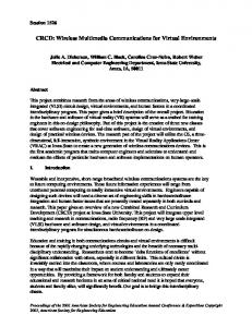
the cameras is minimized. In Section V, we prove that the MLS problem is NP-hard by formulating it as an equivalent binary program. Consequently, we present a randomized approximation algorithm, which produces a solution ≤ 𝑂𝑃 𝑇 + 𝑐𝑚𝑎𝑥 /𝑒, where 𝑂𝑃 𝑇 is the optimal result and 𝑐𝑚𝑎𝑥 is the maximum energy consumed by a camera to send its image to the hub without performing differential coding. II. P ROBLEM F ORMULATION A. Correlation-based Joint Coding and Differential Coding To remove the redundancy among correlated camera sensors, a group of camera sensors as in Fig. 1 can collaboratively compress their data by joint coding and differential coding. Consider a cluster consisting of a multimedia hub with high processing capabilities and 𝑁 ordinary camera sensors {𝑣1 , . . . , 𝑣𝑁 }, where each camera 𝑣𝑖 produces image 𝑋𝑖 . We can perform multi-camera joint coding in the cluster: each camera sends its individual images to the hub, while the hub acts as a single encoder that takes all the collected images as inputs and perform joint coding. We denote the total coding rate of all the images by 𝑅(𝑋1 , ⋅ ⋅ ⋅ , 𝑋𝑁 ). According to Shannon’s source coding theorem, the total coding rate of all nodes within a cluster is lower bounded by the joint entropy of the observations 𝐻(𝑋1 , 𝑋2 , . . . , 𝑋𝑁 ), given by 𝑅(𝑋1 , ⋅ ⋅ ⋅ , 𝑋𝑁 ) ≥ 𝐻(𝑋1 , 𝑋2 , ⋅ ⋅ ⋅ , 𝑋𝑁 ). On the other hand, two camera sensors can also perform inter-camera differential coding with each other. For two images 𝑋𝑖 and 𝑋𝑗 observed by cameras 𝑣𝑖 and 𝑣𝑗 , we can compress 𝑋𝑖 based on the prediction of 𝑋𝑗 . We denote the resulting differential coding rate of 𝑋𝑖 by 𝑅(𝑋𝑖 ∣𝑋𝑗 ), and 𝑅(𝑋𝑖 ∣𝑋𝑗 ) satisfies 𝑅(𝑋𝑖 ∣𝑋𝑗 ) ≥ 𝐻(𝑋𝑖 ∣𝑋𝑗 ), where 𝐻(𝑋𝑖 ∣𝑋𝑗 ) is the conditional entropy of 𝑋𝑖 given the knowledge of 𝑋𝑗 . The conditional entropy can be derived from joint entropy as 𝐻(𝑋𝑖 ∣𝑋𝑗 ) = 𝐻(𝑋𝑖 , 𝑋𝑗 ) − 𝐻(𝑋𝑗 ). Our previous results [4][11] show that the joint entropy for multiple images can be effectively estimated based on the visual correlation between cameras, and this correlation is given by a function of camera settings before the actual images are captured. Specifically, if two cameras 𝐶𝑗 and 𝐶𝑘 can both observe an area of interest 𝑃𝑖 , a spatial correlation coefficient 𝜌𝑗,𝑘 for the observations of 𝑃𝑖 at 𝐶𝑗 and 𝐶𝑘 is derived as (1) 𝜌𝑗,𝑘 = 𝑓 (𝑂𝑗 , 𝑉⃗𝑗 , 𝑂𝑘 , 𝑉⃗𝑘 , 𝑃𝑖 ) which indicates that 𝜌𝑗,𝑘 is a function of the two cameras’ locations (𝑂𝑗 , 𝑂𝑘 ) and sensing directions (𝑉⃗𝑗 , 𝑉⃗𝑘 ) as well as the location of the area of interest 𝑃𝑖 .

2476

B. MinMax Degree Hub Location Problem Consider a camera network modeled by a graph 𝐺 = (𝑉, 𝐸), where 𝑉 is a set of cameras, i.e., 𝑉 = {𝑣1 , 𝑣2 , ...𝑣𝑛 }, and 𝐸 is a set of links. A link (𝑣𝑖 , 𝑣𝑗 ) exists if 𝑣𝑖 and 𝑣𝑗 are within 1-hop range of each other. Definition 1: The degree of a hub h, denoted by 𝑑𝑒𝑔(ℎ), is the total number of hubs (except ℎ) that reside within the 2-hop range of the hub ℎ. To facilitate frequency reuse, the neighboring clusters must be assigned with different channels and the cameras must be able to operate on the channels of their associated clusters. Since the maximum distance between two neighboring clusters is 2-hop distance, by graph coloring theorems [7], this implies that the maximum degree of hubs should be less than the available orthogonal channels to ensure the effectiveness of frequency reuse. For this purpose, we define the MinMax Degree Hub Location Problem as follows Definition 2: MinMax Degree Hub Location Problem (MDHL): given a graph 𝐺 = (𝑉, 𝐸) and a set of potential hub locations 𝐹 = 𝑉 , find a subset 𝐹 ′ ⊆ 𝐹 such that the maximum degree of hubs, maxℎ∈𝐹 ′ (𝑑𝑒𝑔(ℎ)), is minimum, and for all 𝑣𝑖 ∈ 𝑉 , there is at least one hub ℎ ∈ 𝐹 ′ for which (ℎ, 𝑣𝑖 ) ∈ 𝐸. C. Minimum Sum-entropy Camera Assignment Problem After the optimal locations of hubs are determined, our next task is to associate cameras with proper hubs. Since joint coding rate is lower bounded by joint entropy, we formulate the camera assignment task by introducing an optimization problem, namely, Minimum Sum-entropy Camera Assignment Problem (MSCA). Given a hub ℎ, let 𝑎ℎ𝑖 be an indicator variable denoting whether camera 𝑣𝑖 is assigned to ℎ. This value is set to 1 iff 𝑣𝑖 is assigned to 𝑣. We now define Minimum Sum-entropy Camera Assignment Problem as follows Definition 3: Minimum Sum-entropy Camera Assignment Problem (MSCA): given a set of hubs 𝐹 ′ and a set of cameras 𝑉 = {𝑣1 , 𝑣2 , ...𝑣𝑛 } find a function 𝑎 : 𝑉 → 𝐹 ′ assigning each ℎ ∈ 𝐹 ′ in such a way that the total camera 𝑣𝑖 ∈ 𝑉∑to a hub ∪ joint entropy, ℎ∈𝐹 ′ 𝐻( 𝑣𝑖 ∈𝑉 𝑎ℎ𝑖 𝑋𝑣𝑖 ), is minimized. D. Maximum Lifetime Scheduling Problem Given a hub and its member cameras, each hub will generate an order to schedule image collections from its members. Our task is to find the optimal schedule such that the lifetime of the member cameras is maximized. Definition 4: The lifetime of the member cameras is the time duration when all the members of a hub keep alive. Assume that cameras have equal initial energy. The maximization of the lifetime of the cameras in a cluster is equivalent to minimization of the maximum energy consumption of the cameras in this cluster. Let 𝐸𝑡𝑥 (ℎ, 𝑣𝑖 ) denote the energy consumed by 𝑣𝑖 to convey its image to ℎ. 𝐸𝑡𝑥 (ℎ, 𝑣𝑖 ) is a function of {𝑑(ℎ,𝑣𝑖 ) , 𝑅𝑣𝑖 }, in which 𝑑(ℎ,𝑣𝑖 ) is the Euclidean distance between ℎ and 𝑣𝑖 and 𝑅𝑣𝑖 is the predicted differential coding rate of 𝑣𝑖 . Consequently, we formulate the Maximum Lifetime Scheduling Problem (MLS) as follows.

Definition 5: Maximum Lifetime Scheduling Problem (MLS): given a hub ℎ and a set 𝐴ℎ of cameras assigned to ℎ, find a schedule 𝜎 assigning a pair of slots for each cameras to transmit and overhear in such a way that the maximum energy consumption, max𝑣𝑖 ∈𝐴ℎ 𝐸𝑡𝑥 (ℎ, 𝑣𝑖 ), is minimum. In the following sections, we prove that the MDHL problem is NP-complete, while the others are NP-hard. Consequently, approximation and heuristic algorithms are proposed. III. M IN M AX D EGREE H UB L OCATION P ROBLEM In this section, we first prove that MDHL is NP-complete. Next, we formulate MDHL problem as an integer program (IP). Then, we present an approximation algorithm by applying the linear relaxation and random rounding technique, which was originally studied in MAX-2SAT [6] and Covering & Packing problems [8]. A. NP-completeness First, the decision version of the MDHL is as follows. Definition 6: Decision Version of MDHL: given a graph 𝐺 = (𝑉, 𝐸), a set of potential hub locations 𝐹 = 𝑉 , and a positive integer 𝑘, determine if there exists a subset 𝐹 ′ ⊆ 𝐹 with the maximum degree of hubs, maxℎ∈𝐹 ′ (𝑑𝑒𝑔(ℎ)) ≤ 𝑘 such that for all 𝑣 ∈ 𝑉 , there is at least one hub ℎ ∈ 𝐹 ′ for which (ℎ, 𝑣) ∈ 𝐸. Theorem 1: The MDHL is NP-complete. Proof: First, we argue that the decision version of MDHL ∈ NP since given a instance of MDHL, a verification algorithm can efficiently check if each camera has at least one hub in its neighborhood, and if the maximum degree of hubs is 𝑘. Thus, the MDHL belongs to NP. We will now show that the Minimum Dominating Set problem (MDS) is polynomial time reducible to MDHL, i.e., MDS ≤𝑃 MDHL. An instance of MDS is given by a graph 𝐺 = (𝑉 , 𝐸), and a positive integer 𝑘 − 1. The objective is to if there exists a dominating set 𝑉 ′ ⊆ 𝑉 such that determine  𝑉 ′  ≤ 𝑘 − 1 and each element 𝑣 ∈ 𝑉 is a neighbor of at least one element of 𝑉 ′ . Next, we will construct an instance of MDHL problem from an instance ∪ of MDS. We define sets 𝑉 , 𝐹 , 𝐸 as follows: let 𝑉∪ = 𝑉 {𝑢, 𝑓 ′ }, where 𝑢 and 𝑓 ′ are new elements; Let 𝐹 = 𝑉 {𝑓 ′ }; Establish a link between 𝑢 and each element in 𝑉 as well as a link 𝑢 and 𝑓 ′ , and add these links to ∪ between ∪ 𝐸, i.e., 𝐸 = 𝐸 {(𝑢, 𝑓 ′ )} {(𝑢, 𝑣)}𝑣∈𝑉 . Then, the instance of MDHL is given by a graph 𝐺 = (𝑉, 𝐸), a set 𝐹 , and a positive integer 𝑘. We will now prove that the original instance of MDS is a yes instance if and only if the MDHL instance we created is also a yes instance. First, suppose the instance of MDHL has a solution 𝐹 ′ ⊆ 𝐹 with maxℎ∈𝐹 ′ (𝑑𝑒𝑔(ℎ)) ≤ 𝑘. By our construction, 𝑓 ′ is the only 1-hop neighbor of 𝑢, and 𝑢 is the 1-hop neighbor of every element in 𝑉 . It indicates that 𝑓 ′ is the 2-hop neighbor of every element in 𝑉 . Moreover, since 𝑢∈ / 𝐹 ′ , 𝑓 ′ will be added in 𝐹 ′ to cover itself. This implies that 𝑓 ′ is the element in 𝐹 ′ that has the maximum degree 𝑘. Meanwhile, since 𝑉 = 𝑉 − {𝑓 ′ }, this indicates that the

2477

instance of MDS has a dominating set 𝑉 ′ ⊆ 𝑉 of cardinality less than 𝑘 − 1. Next, suppose that there is a dominating set  𝑉 ′ ⊆ 𝑉 with 𝑉 ′  ≤ 𝑘 − 1 in the original MDS instance. By the similar arguments, the degree of the elements in 𝐹 ′ is at most 𝑘 in the constructed MDHL instance. We now have shown that MDS problem can be solved by the proposed construction and an algorithm that solves MDHL. Since our construction takes polynomial time, and MDHL is NP, we can conclude that MDHL is NP-complete. B. IP Formulation of MDHL We first model the MDHL as an integer nonlinear program (INP). Consider a camera network described by a graph 𝐺 = (𝑉, 𝐸) and a set of potential hub locations 𝐹 = 𝑉 . First, we define 1-hop neighborhood and 2-hop neighborhood of a camera 𝑣𝑖 ∈ 𝑉 , respectively. Definition 7: The 1-hop neighborhood of 𝑣𝑖 , denoted by 𝑆𝑖1 , is a set consisting of 𝑣𝑖 and cameras within 1-hop range of 𝑣𝑖 . Definition 8: The 2-hop neighborhood of 𝑣𝑖 , denoted by 𝑆𝑖2 , is a set of cameras within 2-hop range of 𝑣𝑖 . We assign a variable 𝑥𝑖 for each camera 𝑣 ∈ 𝑉 , which is allowed 0/1 values. This variable will be set to 1 iff a hub is placed at the location of 𝑣𝑖 . Consequently, the MDHL problem can be formulated as a Integer Nonlinear Program 𝐼𝑁 𝑃𝑀 𝐷𝐻𝐿 MIN

𝑦

𝑠.𝑡

∑

(2) 𝑥𝑗 ≥ 1, ∀𝑣𝑖 ∈ 𝑉

(3)

𝑥𝑖 𝑥𝑗 ≤ 𝑦, ∀𝑣𝑖 ∈ 𝑉

(4)

𝑗:𝑣𝑖 ∈𝑆𝑗1

∑

𝑗:𝑣𝑖 ∈𝑆𝑗2

𝑥𝑗 ∈ {0, 1},

∀𝑣𝑗 ∈ 𝑉

(5)

The objective function 𝑦 is the maximum degree of all hubs ({𝑣𝑖 ∣𝑥𝑖 = 1}). The first constraint states that each camera 𝑣𝑖 ∈ 𝑉 must reside within the 1-hop neighborhood of at least one hub, whereas the second constraint indicates that the degree of each hub (described in Definition 1) must be less than the maximum value. As the second constraint (4) is quadratic, the formulated integer program 𝐼𝑁 𝑃𝑀 𝐷𝐻𝐿 is not linear. To linearize 𝐼𝑁 𝑃𝑀 𝐷𝐻𝐿 , the quadratic constraint (4) is eliminated by applying the techniques proposed in [5]. More specifically, the product 𝑥𝑖 𝑥𝑗 is replaced by a new binary variable 𝑤𝑖𝑗 , on which several additional constraints are imposed. As a consequence, we can reformulate 𝐼𝑁 𝑃𝑀 𝐷𝐻𝐿 exactly to an integer linear Program 𝐼𝑃𝑀 𝐷𝐻𝐿 by introducing the following linearlization constraints: ∑ 𝑤𝑖𝑗 ≤ 𝑦, ∀𝑣𝑖 ∈ 𝑉 (6) 𝑗:𝑣𝑖 ∈𝑆𝑗2

𝑤𝑖𝑗 ≤ 𝑥𝑖 , 𝑤𝑖𝑗 ≤ 𝑥𝑗 , ∀𝑣𝑖 , 𝑣𝑗 ∈ 𝑉

(7)

𝑤𝑖𝑗 ≥ 𝑥𝑖 + 𝑥𝑗 − 1, ∀𝑣𝑖 , 𝑣𝑗 ∈ 𝑉 𝑤𝑖𝑗 ≥ 0, ∀𝑣𝑖 , 𝑣𝑗 ∈ 𝑉

(8) (9)

and removing the quadratic constraint (4). By relaxing variables 𝑥𝑖 ∈ {0, 1} to 𝑥𝑖 ≥ 0, we get the relaxed linear program

𝐿𝑃𝑀 𝐷𝐻𝐿 consisting of the objective function (2) along with constraints (3), (6), (7), (8), (9), and 𝑥𝑖 ≥ 0, ∀𝑣𝑗 ∈ 𝑉 . C. Randomized Approximation Algorithm Given an instance of MDHL modeled by the integer program 𝐼𝑃𝑀 𝐷𝐻𝐿 , the proposed algorithm (see Algorithm 1) is the following: first solves the relaxed linear program 𝐿𝑃𝑀 𝐷𝐻𝐿 to get an optimal fractional solution, denoted by (x′ , 𝑦 ′ ), where x′ =< x′1 , x′2 , ...x∣𝑉 ∣′ >, and round 𝑥′𝑖 to integers 𝑥𝑖 by a random rounding procedure. This procedure consists of three steps: (i) first set all 𝑥𝑖 to be 0; (ii) then let 𝑥𝑖 = 1 with probability 𝑥′𝑖 and execute this step for log(n)+2 times; (iii) let 𝑥𝑖 = 1 with probability 1/Δ, where Δ is the maximum node degree in the network. The steps (ii) and (iii) yields an integer solution (x, 𝑦), where vector x =< 𝑥1 , 𝑥2 , ..., 𝑥∣𝑉 ∣ >. To ensure (x, 𝑦) is a feasible solution to 𝐼𝑃𝑀 𝐷𝐻𝐿 , the steps (ii) and (iii) are repeated until each camera is the neighbor of at least ∑ one hub, and the integer maximum degree 𝑦 = arg max𝑣𝑖 ∈𝑉 𝑗:𝑣𝑖 ∈𝑆 2 𝑥𝑖 𝑥𝑗 𝑗 satisfies the condition √ that 𝑦 ≤ 𝑟(𝑦 ′ + (1 + 1/Δ)2 ), where 𝑟 = Δ(1 + 𝑚𝑎𝑥(1/𝑦 ′ , 2/𝑦 ′ ))(𝑙𝑜𝑔(𝑛) + 2)2 Algorithm 1 Approximation Algorithm for MDHL 1: 2: 3: 4: 5: 6: 7:

Solve 𝐿𝑃𝑀 𝐷𝐻𝐿 . Let (x′ , 𝑦 ′ ) be the optimum solution. x ← 0, 𝑗 ← 0. while 𝑡 ≤ 𝑙𝑜𝑔(𝑛) + 2 do 𝑥𝑖 ← 1 with probability 𝑝𝑖 ← 𝑥′𝑖 , 𝑡 ← 𝑡 + 1 end while 1 𝑥𝑖 ← 1 with probability 𝑝∑ 𝑖 ← Δ. Repeat lines 3 - 5 Until 𝑥 ≥ 1, ∀𝑣𝑖 ∈ 𝑉 𝑗:𝑣 ∈𝑆 1 𝑗 and 𝑦 = arg max𝑣𝑖 ∈𝑉

∑

𝑖

𝑗

𝑗:𝑣𝑖 ∈𝑆𝑗2

where 𝑟 = Δ(1 + 𝑚𝑎𝑥(1/𝑦 ′ , 8: Return (x, 𝑦)

√

𝑥𝑖 𝑥𝑗 ≤ 𝑟(𝑦 ′ + (1 + 1/Δ)2 ),

2/𝑦 ′ ))(𝑙𝑜𝑔(𝑛) + 2)2

Theorem 2: Let 𝑂𝑃 𝑇 denote the optimal solution of the MDHL problem. The proposed algorithm yields a solution of 𝑂(𝑙𝑜𝑔 2 (𝑛))(𝑂𝑃 𝑇 + (1 + 1/Δ)2 ). Proof: Let 𝑦 ∗ denote the optimal solution to the MDHL problem. Consider any element 𝑣𝑖 ∈ 𝑉 . Its expected degree follows ∑ ∑ ∑ E( 𝑥𝑖 𝑥𝑗 ) = E(𝑥𝑖 )E( 𝑥𝑗 ) = E(𝑥𝑖 ) E(𝑥𝑗 ) 𝑗:𝑣𝑖 ∈𝑆𝑗2

𝑗:𝑣𝑖 ∈𝑆𝑗2

𝑗:𝑣𝑖 ∈𝑆𝑗2

(10) The first equality holds because 𝑣𝑖 is not in its own 2-hop neighborhood 𝑆𝑖2 by Definition 9 and thus 𝑥𝑖 and 𝑥𝑗 are independent. The second equality holds because of linearity of expectation. Applying union bound, we have the probability that an element becomes a hub (i.e., 𝑥𝑖 = 1) when the random rounding is done ∪ 𝑥𝑖 = 1 at round t] ≤ 𝛼𝑥′𝑖 + 1/Δ Pr[𝑥𝑖 = 1] = Pr[ 𝑡≤𝛼+1

where 𝛼 = 𝑙𝑜𝑔(𝑛) + 2. This implies 𝐸(𝑥𝑖 ) ≤ 𝛼𝑥′𝑖 + 1/Δ. Letting 𝛿 = (1 + 1/Δ)2 , we obtain the expected degree of 𝑣𝑖 ∑ ∑ E( 𝑥𝑖 𝑥𝑗 ) ≤ 𝛼 2 𝑥′𝑖 𝑥′𝑗 ≤ 𝛼2 (𝑦 ′ + 𝛿),

2478

𝑗:𝑣𝑖 ∈𝑆𝑗2

𝑗:𝑣𝑖 ∈𝑆𝑗2

∑

which implies E(

𝑗:𝑣𝑖 ∈𝑆𝑗2

𝑥𝑗 ) ≤ Δ𝛼2 (𝑦 ′ + 𝛿).

IV. M INIMUM S UM - ENTROPY C AMERA A SSIGNMENT

Applying Chernoff bound, we obtain the following bound ∑ 𝑥𝑖 𝑥𝑗 ≥ Δ𝜆𝛼2 (𝑦 ′ + 𝛿)] Pr[ 𝑗:𝑣𝑖 ∈𝑆𝑗2

∑

≤ Pr[

𝑥𝑗 ≥ Δ𝜆𝛼2 (𝑦 ′ + 𝛿)] ≤ (

𝑗:𝑣𝑖 ∈𝑆𝑗2

𝑒(𝜆−1) Δ𝛼2 (𝑦′ +𝛿) ) 𝜆𝜆

A. Multi-camera Joint Coding Efficiency Prediction

for 𝜆 > 0. To simplify this bound, suppose 𝜆 > 2𝑒, then ∑ 2 ′ 𝑥𝑖 𝑥𝑗 ≥ Δ𝜆𝛼2 (𝑦 ′ + 𝛿)] ≤ 2−(𝜆−1)Δ𝛼 (𝑦 +𝛿) . Pr[

Given a group of cameras along with their settings, the estimator in [11] gives an upper bound of the joint coding rate by estimating the joint entropy. Next, we gives a brief summary of this estimator followed by a proof of its submodular property. 1) Joint Entropy Estimation: Suppose that 𝑁 cameras (𝑣1 , 𝑣2 , ⋅ ⋅ ⋅ , 𝑣𝑁 ) are deployed on the ground plane, the visual information observed by 𝑣𝑖 is 𝑋𝑖 , and the overall FoV of these cameras is given as 𝒜. The joint entropy of these observations, 𝐻(𝑋1 , ⋅ ⋅ ⋅ , 𝑋𝑁 ), is estimated by two steps: 1) The overall FoV 𝒜 are divided into 𝑀 partitions (𝑃1 , 𝑃2 , ⋅ ⋅ ⋅ , 𝑃𝑀 ), such that each partition is covered by the same set of cameras. For example, the FoVs in Fig. 1 have 6 disjoint partitions. 2) Summing the entropies of all the partitions yields the joint entropy for this group of cameras, i.e,

𝑗:𝑣𝑖 ∈𝑆𝑗2

For 𝜆 < 2𝑒, we can show ∑ (𝜆−1)2 2 ′ Pr[ 𝑥𝑖 𝑥𝑗 ≥ Δ𝜆𝛼2 (𝑦 ′ + 𝛿)] ≤ 𝑒− 4 Δ𝛼 (𝑦 +𝛿) . 𝑗:𝑣𝑖 ∈𝑆𝑗2

Thus, if 𝑦 ′ < 1/𝑒2 , then let 𝜆 = 1 + Pr[

∑

> 2𝑒. We get 2

𝑥𝑖 𝑥𝑗 ≥ Δ𝜆𝛼2 (𝑦 ′ + 𝛿)] ≤ 2−𝛼 ≤ 𝑒−𝛼 ≤

𝑗:𝑣𝑖 ∈𝑆𝑗2

If 𝑦 ′ > 1/𝑒2 , letting 𝜆 = 1 + Pr[

1 𝑦′

∑

√

2 𝑦′

1 . 4𝑛

< 2𝑒, we get

𝑥𝑖 𝑥𝑗 ≥ Δ𝜆𝛼2 (𝑦 ′ + 𝛿)] ≤ 𝑒−

𝛼2 2

≤

𝑗:𝑣𝑖 ∈𝑆𝑗2

1 . 4𝑛

𝐻(𝑋1 , ⋅ ⋅ ⋅ , 𝑋𝑁 ) = 𝐻(𝑃1 ) + ⋅ ⋅ ⋅ + 𝐻(𝑃𝑀 ).

In both of the above cases, summing over all elements 𝑣𝑖 ∈ 𝑉 , we get the probability that some hub has a degree larger than 𝜆𝛼2 𝑦 ′ 1 1 ≤ . (11) Pr[𝑦 ≥ Δ𝜆𝛼2 (𝑦 ′ + 𝛿)] ≤ 𝑛 4𝑛 4 Next we consider the probability that an element 𝑣𝑖 ∈ 𝑉 has no hub in its 1-hop neighborhood at round 𝑗, that is, ∏ ∏ 𝑃 𝑟[𝑥𝑗 = 0 at round j] = (1 − 𝑥′𝑗 ) 𝑗:𝑣𝑖 ∈𝑆𝑗1

≤

∏

𝑗:𝑣𝑖 ∈𝑆𝑗1

′

𝑒−𝑥𝑗 = 𝑒

−

∑

𝑗:𝑣𝑖 ∈𝑆𝑗1 𝑥′ 𝑗:𝑣𝑖 ∈𝑆 1 𝑗 𝑗

≤

1 . 𝑒

The first inequality results from the inequality (1 − 𝑥) ≤ 𝑒−𝑥 , ∀𝑥 ∈ [0, 1]. The second inequality follows the fact that ∑ ′ 𝑗:𝑣𝑖 ∈𝑆𝑗1 𝑥𝑗 ≥ 1. Now, the probability that an element 𝑣𝑖 has no hub in its 1-hop neighborhood after the random rounding is 𝑒−(𝑙𝑜𝑔(𝑛)+2) < 1/4𝑛 Then, by union bound, we get Pr[Some element has no neighboring hub] ≤ 1/4.

In this section, we first prove that the our previously designed estimator for joint coding efficiency is submodular. Next, we show that the MSCA problem is NP-hard and formulate MSCA by introducing the submodular weight set cover problem (SWSC). At last, we propose a polynomial time heuristic algorithm for SWSC.

(13)

The entropy of partition 𝑃𝑖 , 𝐻(𝑃1 ), is defined as follows. Definition 9: Entropy of a Partition. Suppose the group of cameras (𝑣1 , ⋅ ⋅ ⋅ , 𝑣𝑛 ) can observe partition 𝑃𝑖 , and for camera 𝑣𝑘 , its observed visual information about the partition 𝑃𝑖 is denoted by 𝑋𝑘 (𝑃𝑖 ). The entropy of partition 𝑃𝑖 is the joint entropy of the visual information about this partition from the cameras (𝑣1 , ⋅ ⋅ ⋅ , 𝑣𝑛 ), i.e., 𝐻(𝑃𝑖 ) = 𝐻(𝑋1 (𝑃𝑖 ), ⋅ ⋅ ⋅ , 𝑋𝑛 (𝑃𝑖 )). By step 2), we need to calculate the entropy of each partition (𝐻(𝑃𝑖 )) to get the joint entropy for a group of cameras. Before introducing the algorithm for this purpose, we give a key lemma that this algorithm and the followed proof of submodularity rely on. Lemma 1: [11] for cameras 𝑣𝑗 and 𝑣𝑘 in partition 𝑃𝑖 , with observations 𝑋𝑗 (𝑃𝑖 ) and 𝑋𝑘 (𝑃𝑖 ), respectively, assuming that the individual entropies of the observations for 𝑃𝑖 are equivalent, i.e., 𝐻(𝑋𝑘 (𝑃𝑖 )) = 𝐻(𝑋𝑗 (𝑃𝑖 )) = 𝐻(⋅), the conditional entropy of 𝑋𝑗 (𝑃𝑖 ) with the knowledge of 𝑋𝑘 (𝑃𝑖 ) is approximated by

(12)

𝐻(𝑋𝑗 (𝑃𝑖 )∣𝑋𝑘 (𝑃𝑖 )) ≈ (1 − 𝜌𝑗𝑘 ) ⋅ 𝐻(⋅)

(14)

where 𝜌𝑗𝑘 is the correlation coefficient between the observations 𝑋𝑗 (𝑃𝑖 ) and 𝑋𝑘 (𝑃𝑖 ), and it is a normalized symmetric metric satisfying 0 ≤ 𝜌𝑗𝑘 ≤ 1 and 𝜌𝑗𝑘 = 𝜌𝑘𝑗 . 2 ′ The algorithm that calculates the entropy of a partition Pr[each element covered by a hub ∩ 𝑦 ≤ Δ𝜆𝛼 (𝑦 +𝛿)] ≥ 1/2, √ works as follows. First, we calculate a correlation matrix where 𝜆𝛼2 = (1 + max (1/𝑦 ′ , 𝑦2′ ))(𝑙𝑜𝑔(𝑛) + 2)2 . (𝜌𝑗𝑘 )𝑛∗𝑛 for the cameras in the partition based on the methods Observe that both events in this bound can be verified in in [4], and forms a dependency graph among the cameras, polynomial time. If not, we repeat the entire rounding process. in which each camera is only dependent on the camera that The expected number of repetitions is at most 2. is most correlated with it. The joint entropy is estimated by Since the probability of the union of the two undesirable events described in (11) and (12) ≤ 1/2, we get

2479

traversing all the nodes in the graph. For the details of the algorithm, please refer to [11] 2) Submodularity of the Estimated Joint Entropy: Definition 10: A function 𝑓 is called submodular if it satisfies 𝑓 (𝑆) + 𝑓 (𝑇 ) − 𝑓 (𝑆 ∪ 𝑇 ) − 𝑓 (𝑆 ∩ 𝑇 ) ≥ 0. Let 𝑉 = {𝑥1 , ⋅ ⋅ ⋅ , 𝑥𝑛 } be a set of 𝑛 random variables. For a subset of random variables 𝑆 ⊆ 𝑉 , we can define the set function 𝐻(𝑆) as the joint entropy of the variables in 𝑆. We introduce the following lemma for joint entropy. Lemma 2: The entropy function 𝐻(𝑆) is submodular if the conditional mutual information is non-negative. Proof: Consider 𝑆, 𝑇 ⊆ 𝑉 . Denote 𝐶 = 𝑆∩𝑇 , 𝐴 = 𝑆∖𝑇 , 𝐵 = 𝑇 ∖ 𝑆, 𝐷 = 𝑉 ∖ (𝑆 ∪ 𝑇 ). We can express 𝑆 = 𝐴 ∪ 𝐶, 𝑇 = 𝐵 ∪ 𝐶, and 𝑆 ∪ 𝑇 = 𝐴 ∪ 𝐵 ∪ 𝐶. The submodularity condition for 𝐻 can be given as 𝐻(𝑆) + 𝐻(𝑇 ) − 𝐻(𝑆 ∪ 𝑇 ) − 𝐻(𝑆 ∩ 𝑇 ) = 𝐻(𝐴, 𝐶) + 𝐻(𝐵, 𝐶) − 𝐻(𝐴, 𝐵, 𝐶) − 𝐻(𝐶) = 𝐼(𝐴; 𝐵∣𝐶) (15) where 𝐼(𝐴; 𝐵∣𝐶) is the conditional mutual information. Therefore, 𝐻(𝑆) is submodular if 𝐼(𝐴; 𝐵∣𝐶) ≥ 0. To verify the submodularity of the estimated joint entropy, we study if the conditional mutual information from our algorithm is non-negative or not. Lemma 3: Suppose 𝐴, 𝐵, and 𝐶 are three arbitrary sets of visual information collected from camera sensors. The conditional mutual information 𝐼(𝐴; 𝐵∣𝐶) calculated from the proposed algorithm is non-negative. Proof: According to the proposed algorithm, the overall FoV of the cameras in set {𝐴, 𝐵, 𝐶} is divided into several independent partitions, so that the conditional mutual information can be expressed as the sum of the conditional mutual information over each partition. In the following derivation, we study the conditional mutual information of a partition, and the variables below are all defined on a single partition. First, we study the conditional entropy of a variable 𝑥 given a set of variables. (The term ”variable” here stands for the visual information observed by a camera about a partition.) Suppose 𝑆 and 𝑇 are two sets of variables satisfying 𝑆 ⊆ 𝑇 . When estimating joint entropy of a partition in the proposed algorithm, it is assumed that a camera is only dependent on the camera that is most correlated with it. Therefore, based on Lemma 1, we have 𝐻(𝑥∣𝑆) = (1 − 𝜌𝑆𝑥 ) ⋅ 𝐻(⋅) and 𝐻(𝑥∣𝑇 ) = (1 − 𝜌𝑇𝑥 ) ⋅ 𝐻(⋅), where 𝜌𝑆𝑥 is the maximum correlation coefficient between 𝑥 and the variables in 𝑆, 𝜌𝑇𝑥 is the maximum correlation coefficient between 𝑥 and the variables in 𝑇 , and 𝐻(⋅) is the entropy of an individual variable. Since 𝑆 ⊆ 𝑇 , we have 𝜌𝑇𝑥 ≥ 𝜌𝑆𝑥 , and thus we have the following inequation: 𝐻(𝑥∣𝑆) ≥ 𝐻(𝑥∣𝑇 ), if 𝑆 ⊆ 𝑇.

(16) {𝑥𝐴 1 ,⋅⋅⋅

Denote the visual information in set 𝐴 by The conditional entropy 𝐻(𝐴∣𝐵) can be expressed as 𝐻(𝐴∣𝐵) =

𝐻(𝑥𝐴 1 ,⋅⋅⋅

, 𝑥𝐴 𝑁 ∣𝐵)

=

𝑁 ∑ 𝑖=1

, 𝑥𝐴 𝑁 }.

𝐴 𝐴 𝐻(𝑥𝐴 𝑖 ∣𝑥𝑖−1 ⋅ ⋅ ⋅ 𝑥1 𝐵)

(17)

In the same way, the conditional entropy 𝐻(𝐴∣𝐵𝐶) is 𝐻(𝐴∣𝐵𝐶) =

𝑁 ∑

𝐴 𝐴 𝐻(𝑥𝐴 𝑖 ∣𝑥𝑖−1 ⋅ ⋅ ⋅ 𝑥1 𝐵𝐶)

(18)

𝑖=1 𝐴 𝐴 Based on (16), we have 𝐻(𝑥𝐴 ≥ 𝑖 ∣𝑥𝑖−1 ⋅ ⋅ ⋅ 𝑥1 𝐵) 𝐴 𝐴 𝐴 𝐻(𝑥𝑖 ∣𝑥𝑖−1 ⋅ ⋅ ⋅ 𝑥1 𝐵𝐶), and based on (17) and (18), we can derive that 𝐻(𝐴∣𝐵) ≥ 𝐻(𝐴∣𝐵𝐶). As the conditional mutual information satisfies 𝐼(𝐴; 𝐵∣𝐶) = 𝐻(𝐴∣𝐵) − 𝐻(𝐴∣𝐵𝐶), we can obtain that 𝐼(𝐴; 𝐵∣𝐶) ≥ 0, i.e., the conditional mutual information of a single partition is non-negative. Therefore, the overall conditional mutual information, which is the sum of the conditional mutual information over all the partitions, is also non-negative. Combining Lemma 2 and Lemma 3, we conclude that the estimated joint entropy function is submodular.

B. SWSC formulation for MSCA As described in Definition 4, the MSCA problem can be modeled by a binary problem with nonlinear objective function, which is a known NP-hard problem. In this subsection, we formulate the MSCA problem by defining the submodular weight set cover problem (SWSC). Towards this, we model the camera assignment choices for a hub as a collection of subsets of cameras within the hub’s 1-hop neighborhood, with each subset associated with a submodular weight, which is the joint entropy of the cameras in this subset. Consider a hub ℎ. We adopt the following notations. 𝑒 ∙ 𝑆ℎ : set of cameras exclusively covered by ℎ. 𝑐 ∙ 𝑆ℎ : set of cameras commonly covered by ℎ and other hubs. 𝑐 𝑐 ∙ 𝑃 (𝑆ℎ ): power set of 𝑆ℎ , which is a set of all subsets of 𝑐 𝑆ℎ , including empty set and 𝑆ℎ𝑐 itself. ∙ 𝐴ℎ : = ∪ assignment choice set of ℎ, 𝐴ℎ {𝑆ℎ𝑒 𝑊 }𝑊 ∈𝑃 (𝑆ℎ𝑐 ) . Apparently, each hub ℎ may have exponentially many choices (i.e., ∣𝐴ℎ ∣ = ∣𝑃 (𝑆ℎ𝑐 )∣ ≤ 2∣𝑉 ∣ ), and we aim to choose one choice (subset) for each hub so that the total costs of the choices (the total entropy of the subsets) is minimum. Now, the submodular weight set cover problem (SWSC) is formally defined as follows. Definition 11: Submodular weight set cover problem (SWSC): given a universe 𝑈 of 𝑛 elements, 𝑘 centers, a collection of assignment choice sets of centers, 𝑆 = {𝐴ℎ𝑖 }𝑘𝑖=1 , and a submodular weight function 𝑐 : 2∣𝐴ℎ ∣ → ℛ+ , find a minimum weight subcollection 𝑆 ′ ⊆ 𝑆 of cardinality 𝑘, which covers all elements in 𝑈 . C. Polynomial Time Heuristic Algorithm To solve the conventional set cover problem [3], the greedy approach applies: iteratively select the set that minimizes the ratio of the set’s cost to the number of new elements it covers, until all elements are covered. However, to solve SWSC problem, this algorithm can not be done in polynomial time by simply enumerating all potential sets at each iteration, because as described previously, each instance of the SWSC

2480

problem may have an exponential number of subsets. To address this problem, we design a heuristic algorithm that makes at most a constant number of calls to a polynomial time subroutine. By this, we prove that the proposed algorithm runs in polynomial time. Before presenting the algorithm, we introduce the following theorem. Theorem 3: (Schrijver [9]) Given a finite set 𝑉 and a submodular set function 𝑓 on set 𝑉 , a subset 𝑆 ∗ of 𝑉 with the minimum 𝑓 (𝑆 ∗ ) can be found by a polynomial number of calls of function 𝑓 . We now present the proposed algorithm in details (see Algorithm 2). Given a set of cameras 𝑉 and a set of hubs, ℱ = {ℎ𝑖 }𝑘𝑖=1 . At each iteration, we find the set with the minimum average cost from the set 𝐴ℎ𝑖 of each hub ℎ𝑖 , and select the best set among all hubs. If a hub ℎ𝑖 ’s subset is selected, we remove ℎ𝑖 from the collection ℱ and update the assignment choice sets {𝐴ℎ𝑖 }ℎ𝑖 ∈ℱ for the remaining hubs. By analyzing Algorithm 2, we have the following lemma. Lemma 4: Given 𝑘 hubs, the proposed algorithm takes 𝑘 iterations to select 𝑘 disjoint sets (assignment choices) such that each camera is assigned to exactly one hub. Since in each iteration, we need a subroutine that finds a set 𝑆 ∗ ∈ 𝐴ℎ minimizing the ratio of 𝐻(𝑆)/ ∣𝑆 ∩ 𝐶∣, we prove that the proposed algorithm runs in polynomial time by proving the following Lemma. Lemma 5: Using binary search, the set 𝑆 minimizing ratio 𝐻(𝑆)/ ∣𝑆 ∩ 𝐶∣ can be found in polynomial time. Proof: Assume the minimum ratio 𝐻(𝑆)/ ∣𝑆 ∩ 𝐶∣ is 𝑎. We can verify if this assumption holds by testing whether the minimum value of 𝐻(𝑆) − 𝑎 ∣𝑆 ∩ 𝐶∣ is less than 0. Since the sum of submodular and modular functions is a submodular function, function 𝐻(𝑆)−𝑎 ∣𝑆 ∩ 𝐶∣ is submodular since 𝐻(𝑆) is submodular and −𝑎 ∣𝑆 ∩ 𝐶∣ is modular. Moreover, it is easy to verify that given an arbitrary set 𝑆, its entropy 𝐻(𝑆) can be calculated in polynomial time by the designed estimator. Consequently, by Theorem 3, the minimum value of 𝐻(𝑆) − 𝑎 ∣𝑆 ∩ 𝐶∣ can be found in polynomial time. Algorithm 2 Heuristic Algorithm for SWSC 1: 𝐶 ← ∅, ℱ = {ℎ𝑖 }𝑘𝑖=1 2: while ℱ ∕= ∅ do 3: {ℎ∗ , 𝑠∗ℎ } ← arg minℎ∈ℱ {min𝑠ℎ ∈𝐴ℎ 𝐻(𝑠ℎ )/ ∣𝑠ℎ ∩ 𝑉 ∣}. 4: 𝐶 ← 𝐶 ∪𝑠∗ℎ , ℱ ← ℱ ∖ℎ∗ , 𝑉 = 𝑉 ∖𝑠∗ℎ , updates 𝐴ℎ𝑖 , ∀ℎ𝑖 ∈ ℱ 5: end while

V. M AXIMUM L IFETIME S CHEDULING P ROBLEM In this section, we first prove that the MLS problem is NPhard by formulating it as an equivalent binary program. Consequently, we present a randomized approximation algorithm, which produces a solution ≤ 𝑂𝑃 𝑇 + 𝑐𝑚𝑎𝑥 /𝑒 in expectation, where 𝑐𝑚𝑎𝑥 is the maximum energy consumed by a camera to send its image to the hub without performing differential coding. A. IP Formulation for MSL Given a hub ℎ and a set 𝐴 of cameras assigned to it. To save energy, we let the transmission range of each camera 𝑣𝑖 ∈ 𝐴 be

the distance between 𝑣𝑖 and hub ℎ, denoted by 𝑑𝑖ℎ . For each camera 𝑣𝑖 ∈ 𝐴, let 𝑁𝑖 denote a set of cameras within 𝑣𝑖 ’s transmission range, and let 𝑋𝑖 denote the image gathered by 𝑣𝑖 . We assign two variables 𝑥𝑖 and 𝑦𝑗𝑖 for each camera 𝑣𝑖 ∈ 𝐴, which are allowed 0/1 values. 𝑥𝑖 is set to 1 iff 𝑣𝑖 sends its image without overhearing and performing differential coding. 𝑦𝑗𝑖 is set to 1 iff 𝑣𝑖 overhears 𝑣𝑗 ’s transmission and encodes its image 𝑋𝑖 conditional on 𝑣𝑗 ’s image 𝑋𝑗 . In particular, 𝑦𝑖𝑖 is set to 1 iff 𝑣𝑖 does not overhear anyone’s transmission. Consequently, we formulate the maximum lifetime scheduling problem as an integer program 𝐼𝑃𝑀 𝑆𝐿 . MIN 𝑠.𝑡

𝑧

∑

(19) 𝑥𝑗 ≥ 1, ∀𝑣𝑖 ∈ 𝐴

(20)

𝑦𝑗𝑖 = 1, ∀𝑣𝑖 ∈ 𝐴

(21)

𝑗:𝑣𝑖 ∈𝑁𝑗

∑

𝑗:𝑣𝑖 ∈𝑁𝑗

𝑦𝑗𝑗 = 𝑥𝑗 ≥ 𝑦𝑗𝑖 ∀𝑣𝑖 , 𝑣𝑗 ∈ 𝐴 (22) ∑ 2 𝑦𝑗𝑖 𝐻(𝑋𝑖 ∣𝑆𝑗 )𝑑𝑖ℎ ≤ 𝑧, ∀𝑣𝑖 ∈ 𝐴 (23) 𝑗:𝑣𝑖 ∈𝑁𝑗

𝑥𝑗 , 𝑦𝑗𝑖 ∈ {0, 1}, ∀𝑣𝑗 , 𝑣𝑖 ∈ 𝑉

(24)

The objective function 𝑧 is the maximum energy consumption of all cameras in 𝐴. The constraint (20) ensures that each camera has at least one camera to overhear. The constraint (21) states that each camera only overhears once. The equality of the constraint (22) indicates if 𝑣𝑖 decides to send its image without performing differential coding, it will not overhear at all, whereas the inequality 𝑥𝑗 ≥ 𝑦𝑗𝑖 states that 𝑣𝑗 must send its image before 𝑣𝑖 can overhear 𝑣𝑗 ’s transmission. The constraint (23) ensures that the energy consumed by each camera 𝑣𝑖 to send its compressed image of 𝐻(𝑋𝑖 ∣𝑋𝑗 ) bits over the distance 𝑑𝑖ℎ is less than the maximum value 𝑧. Slightly different from the notation of the classic information theory, we let 𝐻(𝑋𝑖 ∣𝑋𝑖 ) = 𝐻(𝑋𝑖 ), which means that a camera only sends its original image if it does not overhear anyone’s transmission, i.e., 𝑦𝑖𝑖 = 1. By relaxing the binary variables 𝑥𝑗 , 𝑦𝑗𝑖 ∈ {0, 1} to 𝑥𝑗 , 𝑦𝑗𝑖 ∈ [0, 1], we get the relaxed linear problem 𝐿𝑃𝑀 𝐿𝑆 . Algorithm 3 Approximation Algorithm for MLS 1: 2: 3: 4: 5: 6: 7: 8: 9: 10:

Solve 𝐿𝑃𝑀 𝑆𝐿 . Let (x′ , y′ , 𝑧 ′ ) be the optimum solution. x ← 0, 𝑗 ← 0. 𝑥𝑖 ← 1 with probability 𝑥′𝑖 , 𝑦 𝑖𝑖 ← 1 if 𝑥𝑖 = 1 ′ For each 𝑣𝑖 ∈ 𝐴 with 𝑥𝑖 = 0, find 𝑂𝑗 = {𝑣𝑖 ∣𝑦𝑗𝑖 ∕= 0, 𝑥𝑖 = 1} if 𝑆𝑖 ∕= ∅ then 𝑣𝑗 ∗ = arg min𝑣𝑗 ∈𝑂𝑖 𝐻(𝑋𝑖 ∣𝑋𝑗 )𝑑2𝑖ℎ and 𝑦 𝑗 ∗ 𝑖 ← 1 else 𝑥𝑖 ← 1 and 𝑦 𝑖𝑖 ← 1 end if Return (x, y, 𝑧)

B. Approximation Algorithm for MSL In this subsection, we propose an approximation algorithm based on the similar random rounding techniques presented

2481

in section III. More specifically, we call a camera 𝑣𝑖 as a broadcaster if its variable 𝑥𝑖 = 1, and as a listener if 𝑥𝑖 = 0. The proposed algorithm works as follows (see Algorithm 3): initially, let all cameras 𝑣𝑖 ∈ 𝐴 stay as listeners, after solving the linear problem 𝐿𝑃𝑀 𝐿𝑆 , which yields an optimal fractional solution (x′ , y′ , 𝑧 ′ ), let each camera 𝑣𝑖 ∈ 𝐴 become a broadcaster with probability 𝑥′𝑖 . Otherwise, the cameras stay as listeners. For each listener 𝑣𝑖 , find all broadcasters 𝑣𝑗 ∈ 𝐴 ′ , and if such broadcasters exist, assign that have nonzero 𝑦𝑗𝑖 the listener 𝑣𝑖 to the broadcaster having the smallest cost 𝐻(𝑋𝑖 ∣𝑆𝑗 )𝑑2𝑖ℎ , otherwise let 𝑣𝑖 become a broadcaster itself. Theorem 4: Let 𝑂𝑃 𝑇 denote the optimal solution of the MLS problem. The solution of the proposed algorithm is at most 𝑂𝑃 𝑇 + 𝐻(𝑋)𝑑2𝑚𝑎𝑥 /𝑒 in expectation, where 𝑑𝑚𝑎𝑥 is the maximum distance between a camera and its assigned hub. Proof: First, by the pseudo code in Algorithm 2, we can verify that the proposed algorithm produces a feasible solution, that is, when the algorithm is done, every camera is either a broadcaster or a listener. To get the expected energy of a camera 𝑣𝑖 , we establish an overhearing list 𝐿𝑖 for 𝑣𝑖 , ′ ∕= 0). These which consists of 𝑖’s potential broadcasters (𝑣𝑗 ∣𝑦𝑗𝑖 potential broadcasters are arranged in an increasing order of the cost 𝑐𝑗𝑖 = 𝐻(𝑋𝑖 ∣𝑋𝑗 )𝑑2𝑖ℎ , 𝑗 = 1, 2, ..., 𝑛, where 𝑛 is the list length. By this way, we have ′ ′ ′ = 𝑥′1 , 𝑦2𝑖 = 𝑥′2 , ..., 𝑦𝑛𝑖 = 𝑥′𝑛 . 𝑦1𝑖

(25)

The above equalities hold because to reduce the cost of a listener, it has to listen to the broadcaster that leads to the smallest cost as possible as it can. Now, we get the probability that a camera 𝑣𝑖 has no broadcaster in its overhearing list. ∑ ∏ ∏ − 𝑥′ ′ −𝑥′𝑗 𝑗:𝑣𝑗 ∈𝐿𝑖 𝑗 (1 − 𝑥𝑗 ) ≤ 𝑒 =𝑒 𝑝𝑖 = 𝑗:𝑣𝑗 ∈𝐿𝑖

∑

𝑗:𝑣𝑗 ∈𝐿𝑖

1 𝑗:𝑣𝑖 ∈𝑁𝑗 = 𝑒 = 𝑒 The first inequality results from the inequality (1 − 𝑥) ≤ 𝑒−𝑥 , ∀𝑥 ∈ [0, 1]. The first equality in the second line holds because of (25). The last equality follows the fact that ∑ ′ 𝑗:𝑣𝑖 ∈𝑁𝑗 𝑦𝑗𝑖 = 1. According to the algorithm, if 𝑣𝑖 is a broadcaster, an event that occurs with probability 𝑥′𝑖 , then 𝑣𝑖 has a cost 𝑐𝑖𝑖 . Otherwise, 𝑣𝑖 overhears the first camera in the list. If this camera is a broadcaster, an event that occurs with probability ′ ′ 𝑦1𝑖 , then 𝑣𝑖 has a cost 𝑐1𝑖 . If the first camera is not 𝑦𝑖𝑖 a broadcaster and the second is, an event that occurs with ′ ′ (1 − 𝑦1𝑖 ′ )𝑦2𝑖 , 𝑣𝑖 has a cost 𝑐2𝑖 , and so on. probability 𝑦𝑖𝑖 If there exists no broadcasters in the list, an event that occurs with probability 𝑝𝑖 , then 𝑣𝑖 becomes a broadcaster and has a cost less than 𝑐𝑚𝑎𝑥 = 𝐻(𝑥)𝑑2𝑚𝑎𝑥 . By the fact ∑ ′ ′ 𝑗:𝑣𝑖 ∈𝑁𝑗 𝑦𝑗𝑖 𝑐𝑗𝑖 ≤ 𝑧 ≤ 𝑂𝑃 𝑇 , the expected cost of a camera has an upper bound −

′ 𝑦𝑗𝑖

′ ′ ′ ′ ′ ′ ′ 𝑐𝑖𝑖 + 𝑦𝑖𝑖 𝑦1𝑖 𝑐1𝑖 + 𝑦𝑖𝑖 𝑦2𝑖 𝑐2𝑖 + ... + 𝑦𝑖𝑖 𝑦𝑛𝑖 𝑐𝑛𝑖 + 𝑝𝑖 𝑐𝑚𝑎𝑥 𝑦𝑖𝑖 ∑ ′ ≤ 𝑦𝑗𝑖 𝑐𝑗𝑖 + 𝑐𝑚𝑎𝑥 /𝑒 ≤ 𝑂𝑃 𝑇 + 𝐻(𝑥)𝑑2𝑚𝑎𝑥 /𝑒. 𝑗:𝑣𝑖 ∈𝑁𝑗

VI. P ERFORMANCE E VALUATION In this section, we evaluate the performance of the proposed image gathering schemes. First, we evaluate the effectiveness of the estimator that predicts the joint coding and different coding efficiency. Then, we study the efficiency of the proposed network deployment approach that consists of the proposed hub placement and camera assignment algorithms. In the end, we evaluate the differential coding-based scheduling algorithm in terms of energy saving. A. Validation of the Coding Efficiency Prediction Since the entropy-based estimator provides predicted coding efficiency for the proposed visual correlation-based schemes, we need to validate its effectiveness by comparing the estimated coding efficiency with the actual coding efficiency from practical coding experiments. Since the performance of the estimator for predicting joint coding efficiency was tested in [11], we only need to validate its capability to predict the differential coding efficiency. Suppose image 𝑋𝑖 is coded based on the prediction of image 𝑋𝑗 , and we can define an estimated differential coding efficiency as 𝐷 𝜂𝐻 =1−

𝐻(𝑋𝑖 ∣𝑋𝑗 ) 𝐻(𝑋𝑖 )

(26)

where 𝐻(𝑋𝑖 ∣𝑋𝑗 ) is the theoretical coding rate of differential coding. This metric predicts the percentage of rate savings of differential coding compared to individual coding. The actual differential coding efficiency is calculated by replacing the entropy terms in (26) with the corresponding coding rates from our coding experiment. In our experiment, we deploy a number of camera nodes in a field and record each camera’s FoV parameters. We deploy the cameras in two scenes, an indoor scene and an outdoor one. For each scene, we let each camera capture an image at the same time, and perform coding experiments on the observed images. The H.264 Multi-View Coding (MVC) coding standard with reference software version JMVC 2.5 [1] is used here. We test the differential coding efficiency between 2 images, and the joint coding efficiency among 3 images. Comparisons of the estimated coding efficiency and the actual coding efficiency are plotted in Fig. 2. It can be found that the actual coding efficiency is approximately proportional to the estimated coding efficiency. Therefore, the proposed entropy-based estimation method can be used to predict the performance of multi-camera joint coding and inter-camera differential coding. B. Efficency of the Combined Network Deployment Scheme In this section, we evaluate the joint performance of the proposed hub placement and camera assignment algorithms in terms of spectrum utilization enhancement and image compression efficiency. Specifically, we compare this combined scheme with the DMCP protocol in our previous work [11], in terms of the maximum hub degree and the overall coding rate. The DMCP selects a set of clusters that minimizes the total coding rate of all clusters under the assumption that the

2482

100

20

15

10

5

Total Coding Rate Ratio Hub Degree Ratio Robustness Ratio

1.1

80

1 0.9 0.8 0.7 0.6 0.5 0.4

Fig. 2.

10 20 30 Estimated coding efficiency (%)

0.1 1

40

Estimation of coding efficiency.

70 60 50 40 30 20

0.3

10

0.2

0

Optimal DC Schedule Approx. DC Schedule Non−DC schedule

90

Energy Consumption

Differential coding (scene 1) Differential coding (scene 2) Joint coding (scene 1) Joint coding (scene 2)

Network Deployment Efficiency (%)

Actual coding efficiency (%)

25

2

3

4

5

6

7

Network Instance

Fig. 3. Throughput Oriented Deployment verse Spectrum Unawared Deployment

number of non-overlapped channels is sufficiently large to support parallel transmissions. Here, we consider a WMSN network of 50 camera sensors uniformly distributed in a 100𝑚 × 100𝑚 region. In Fig. 3, we measure the maximum hub degree and the total coding rate produced by each scheme under 7 randomly generated network topologies, and calculate the ratios of the measurements of the combined scheme to those produced by the DMCP. We observe that the hub degree ratio is less than 0.6, which indicates the combined solution requires much less orthogonal channels than the DMCP, and thus has capabilities to tolerate the significant reduction of the available channels because of interferences caused by other wireless networks. Moreover, we observe that the total coding rate ratio is almost 1, which implies that both schemes achieve comparable compression efficiency. It is also seen in Fig. 3 that the robustness ratio is less than 1, which means that compared with the DMCP, the combined scheme has fewer cameras that are covered by more than one hub. C. Energy Saving of Differential Coding-based Scheduling We now investigate the performance of the proposed differential coding-based scheduling. Here, we consider a cluster, in which 10 camera sensors are uniformly distributed within the transmission range of the hub. In Fig. 4, we randomly generate 5 cluster instances and measure the maximum energy consumption per image of the cameras yielded by our proposed randomized algorithm, whose results are averaged after 10 independent repetitions. As benchmarks, the optimal schedules are also found by the Branch and Bound algorithm, an enumeration based technique. We observe that the proposed scheduling scheme leads to a considerable energy reduction, compared with the conventional TDMA-based scheduling. This is due to the fact that the differential coding-based scheduling allows cameras to remove the redundancy between each other, thus reducing the bits sent to the hub. In addition, we observe that the results of the proposed scheduling scheme are comparable with the optimal ones. VII. C ONCLUSIONS In this paper, we address three fundamental problems involved in the process of image gathering. More specifically, the MDHL problem aims to find the optimal hub locations such that the required number of orthogonal channels for frequency reuse is minimum. To solve this problem, a near

0 0

1

2

3

4

5

6

Topology Instance

Fig. 4. Energy Saving by Differential Codingbased (DC) Scheduling

optimal approximation algorithm is proposed, which yields an 𝑂(𝑙𝑜𝑔 2 (𝑛)) approximation factor. With the knowledge of the hub locations, the MSCA problem is dedicated to associate cameras with proper hubs such that the overall compression efficiency is maximized. To address this problem, a heuristic algorithm is presented based on the greedy scheme and a submodular function subroutine. In the end, a novel differential coding-based scheduling scheme is proposed with an objective to maximize the sensor’s lifetime. Experiments and simulations show that the proposed image gathering schemes effectively and efficiently improve the spectrum utilization and the image compression efficiency. ACKNOWLEDGEMENTS This work was supported by the US National Science Foundation (NSF) under Grant No. ECCS-0701559. R EFERENCES [1] JMVC Reference Software JMVC 2.5. Available: http://ftp3.itu.int/ av-arch/jvt-site/2008 10 Busan/JVT-AC207.zip. [2] I. F. Akyildiz, T. Melodia, and K. R. Chowdhury. A survey on wireless multimedia sensor networks. Elsevier Computer Networks Journal, 51(4):921–960, 2007. [3] V. Chvatal. A greedy heuristic for the set covering problem. Mathematics of Operations Research, 4(3):233–235, 1979. [4] R. Dai and I. F. Akyildiz. A spatial correlation model for visual information in wireless multimedia sensor networks. IEEE Transactions on Multimedia, 11(6):1148–1159, Oct. 2009. [5] R. Fortet. Applications de lalgebre de boole en recherche operationelle. Revue Francaise de Recherche Operationelle, 4:17–26, 1960. [6] M. X. Goemans and D. P. Williamson. New 3/4-approximation algorithms for the maximum satisfiability problem. SIAM Journal On Discrete Mathematics, 7(4):656–666, 1994. [7] R. Gould. Graph Theory. Benjamin-Cummings, 1988. [8] P. Raghavan and C. D. Thompson. Randomized rounding: a technique for provably good algorithms and algorithmic proofs. Combinatorica, 7:365–374, 1987. [9] A. Schrijver. A combinatorial algorithm minimizing submodular functions in strongly polynomial time. Journal of Combinatorial Theory, 80(2):346–355, 2000. [10] R. Wagner, R. Nowak, and R. Baraniuk. Distributed image compression for sensor networks using correspondence analysis and super-resolution. In IEEE International Conference on Image Processing, pages 597–600, 2003. [11] P. Wang, R. Dai, and I. F. Akyildiz. Collaborative data compression using clustered source coding for wireless multimedia sensor networks. In Proc. IEEE INFOCOM, Mar. 2010.

2483