Visual Debugging for Stream Processing Applications Wim De Pauw, Mihai Leția, Buğra Gedik, Henrique Andrade1, Andy Frenkiel, Michael Pfeifer, Daby Sow IBM T.J. Watson Research Center Hawthorne NY 10532, USA {wim, mletia, bgedik, afrenk, pfeifer, sowdaby}@us.ibm.com
Abstract. Stream processing is a new computing paradigm that enables continuous and fast analysis of massive volumes of streaming data. Debugging streaming applications is not trivial, since they are typically distributed across multiple nodes and handle large amounts of data. Traditional debugging techniques like breakpoints often rely on a stop-the-world approach, which may be useful for debugging single node applications, but insufficient for streaming applications. We propose a new visual and analytic environment to support debugging, performance analysis, and troubleshooting for stream processing applications. Our environment provides several visualization methods to study, characterize, and summarize the flow of tuples between stream processing operators. The user can interactively indicate points in the streaming application from where tuples will be traced and visualized as they flow through different operators, without stopping the application. To substantiate our discussion, we also discuss several of these features in the context of a financial engineering application. Keywords: Visualization, debugging, streaming applications, performance analysis, tracing.
1 Introduction Stream processing is a new emerging computing paradigm with applications in various areas such as environment monitoring, financial trading, business intelligence and healthcare [1]. This paradigm enables continuous and immediate analysis of massive volumes of streaming data. In contrast with traditional data analysis approaches, stream computing does not require data to be persisted before being analyzed. It allows for data to be analyzed while in motion, by going through a mostly static set of long-standing queries that constitute the core of stream processing applications. While data stream processing systems are substantially different from traditional database-centric analysis systems, developers are confronted with familiar challenges 1
Currently working at Goldman Sachs. Henrique can be reached at
[email protected].
and goals, i.e. the identification of the causes for incorrect or missing results, the identification of errors in the input data, the understanding of performance degradation issues, including exhaustion of resources, and the coping with design flaws, among others. However, the nature of streaming applications prevents classical debugging approaches to fully achieve these debugging goals. Indeed, typical streaming applications can be highly distributed to handle large data throughput and low latency requirements. This distribution of computation yields numerous possible data paths in an application thus complicating the identification of causes of problems. Furthermore, in a streaming environment where data is constantly in motion, it is quite hard, if not impossible, to capture a complete and globally consistent view of the input data streams and the application state. While breakpoints may be useful for debugging single node applications, they are insufficient for streaming applications for the following reasons. First, the cause and the manifestation of an error may be situated at different locations. Second, halting the execution on one node often has a “train wreck” effect on streaming applications, disturbing the relative order of events throughout the application. Finally, the large amounts of data that are typically processed in streaming applications make manual inspections of individual tuples sent across operators quite impractical and difficult without proper tooling. This paper presents a new visual and analytic environment to support large-scale application understanding, including specific features for debugging, performance analysis, and troubleshooting. Our environment consists of several visualization methods to study, characterize, and summarize the flow of tuples between streaming operators as part of System S [2], a large-scale stream-processing platform developed at IBM Research. We demonstrate several techniques for tracing and visualizing the data flow of streaming applications that enable the developer to understand the application's runtime behavior and more effectively locate and diagnose typical problems. The proposed environment allows the user to recreate these data flows in a temporally accurate fashion. The user can also interactively indicate points in the streaming application from where tuples will be traced and visualized as they flow through different operators, without stopping the application. The tracing and visualizations described here are intended to be used in concert with the existing debugging techniques described in our earlier work [3, 4, 5], thereby enabling the developers to apply the existing techniques when they can be the most effective. To substantiate our discussion, we organize the presentation of the features of our visualization tool in the context of a simple, yet real-world inspired financial engineering application. In Section 2, we describe the programming model used by System S, the distributed stream computing platform on which we have implemented our visual debugging concepts. After a comparison with related work in Section 3, we propose the fundamental model of the data dependencies in Section 4. We describe the visual syntax of our tool in Section 5. Section 6 illustrates the new features with real-world debugging scenarios. Section 7 highlights major design points in our prototype and we conclude with Section 8.
2 SPADE and System S in a Nutshell SPADE [6] is the programming language used for developing stream processing applications on System S [2], a distributed stream processing platform developed by IBM Research. We briefly describe some of the programming language features, focusing on the aspects that are directly related to the visualization capabilities described in this work: Flow composition: The SPADE language provides composition capabilities that are used to create data flow graphs out of basic analytical units called operators. Operators are composed into data flow graphs via stream connections. This is called static flow composition, where the topology of the data flow graph is constructed at application development time and does not change at runtime. The language also supports dynamic flow composition, where connections are established at runtime, based on conditions specified at development time and availability of matching streams at runtime. In addition to these, SPADE also supports hierarchical flow composition via composite operators. A composite operator encapsulates a data flow graph as an operator, which enables development of large-scale streaming applications. Flow manipulation: SPADE provides a type system and an expression language. They provide the basic constructs for expressing flow manipulations as custom functions and operators. A standard set of operators that are parameterizable using SPADE expression language, as well as a large set of built-in functions are also provided. The standard set of operators include basic relational manipulations such as selection, projection, aggregation, join, and sort, as well as common utilities such as buffering, throttling, splitting, merging, etc. Fundamental abstractions, such as windowing, punctuations, output functions, and operator parameters, among others are provided to facilitate flexible and powerful flow manipulations. The language also provides a set of edge adapters to connect operators to external sources and sinks, for ingesting external stream data and producing results to be consumed by external applications, respectively. Extensible analytics: The SPADE language supports extensibility through toolkits. A toolkit is a set of reusable operators and functions [7]. The language can be extended with new operators, written in general-purpose programming languages, such as C++ and Java. Such operators can be type generic and parametrizable. In other words, they can potentially operate on any type (as in a Projection operator in relational algebra) and can be customized using SPADE’s expression language (as in defining a match condition for a relational Join operator). This enables third parties to provide cross-domain as well as domain-specific toolkits of operators and functions, which encapsulate various streaming analytics from a wide range of application domains [1]. Distributed execution: The SPADE language provides various configuration options that influence the mapping of the logical data flow graph to a physical one, which can be deployed on a set of distributed hosts. For instance, the language can be used to express operator fusion constraints, which influence how operators are grouped into partitions that map to OS processes. Similarly, it can be used to specify
partition placement constraints, which influence how processes representing the partitions are mapped to hosts. Ex-location and isolation constraints at the partition and host-level are also supported. These constraints can be used to express detailed requirements [8] in terms of how an application executes on the distributed platform. The SPADE language can also be used to specify threading and queueing configurations, controlling the data processing behavior within an operator and of an input port, respectively. System S provides the runtime platform on which SPADE applications run. It provides management services such as scheduling, security, job management and monitoring, fault-tolerance services, dynamic stream traffic routing, to name a few. It also provides a high-performance communication substrate for SPADE applications, which makes available highly efficient transport capabilities for cross-process and cross-node communication; including some of the capabilities we make use of for visualization purposes, such as exposed performance metrics and tuple tagging.
3 Related Work There are several bodies of literature related to this work, ranging from debugging systems to streaming data provenance tracking systems. Causeway [9] is a debugging system that allows developers to debug message-passing distributed systems. Using Causeway, the developer can observe the connection between the function call stack and the message passing mechanism. However, debugging is done postmortem, by processing offline traces that have been generated at runtime. Our tool allows live debugging and is able to reconfigure the tracing, based on intermediate results, which might already have attracted the attention of a developer. The authors of Causeway state that their system generates large quantities of debugging data, but they do not tackle the problem of narrowing the tracing space. Our tool uses execution slices to only trace the part of the system that is under observation, as we will describe later. Causeway is able to capture dependencies between an incoming message and one or more outgoing messages that were caused by it, but does not support the model where several incoming messages are aggregated into an outgoing message. Our debugging environment is able to aggregate tuples from the same or different input ports to output a single resulting tuple. To present the results, the Causeway tool uses textbased representations, comparable to the ones found in traditional debuggers while our tool provides the user with graphical models of entities in System S and their interactions. Finding causalities between input and output data has been the focus of research in data provenance. In the context of stream computing, data provenance has received only a limited amount of attention, such as in the work of Vijayakumar et al. [10] Their work focuses on identifying and storing dependencies among streams (by encoding, as a tree, the IDs of ancestor streams of a derived stream), rather than the data dependencies for individual stream tuples. In our earlier work [11, 12] we proposed efficient techniques to track data and explored a model-based solution for data provenance in stream computing platforms. In a nutshell, our approach compresses the meta-data needed to track data provenance into a set of rules capturing
input-output dependencies. The system that we developed is limited to backward provenance queries. Furthermore, the capture of provenance meta-data is severely limited by the capacity of the underlying storage system where the traces are persisted. Our previous work in problem determination for Web Services uses message tagging [13] as well as semantic correlations between messages [14] to discover the data flow in business applications. Aguilera et al. [15] propose a method that treats the distributed components as black boxes. They infer causal paths from the observed messages by finding nested calls for RPC-style communication or by applying signal processing techniques that rely on the time variance between request and response messages. However, all these techniques that help with problem determination in distributed debugging are hard to apply to stream processing, because the volume ingested streaming data makes the implementation of these techniques impractical, if not impossible. The Streams Debugger [5] enables a developer to inspect individual tuples in a SPADE application, by setting breakpoints and tracepoints on an operator's input or output ports. At a breakpoint, the flow of tuples on the stream connection is suspended, enabling the developer to examine, and optionally update, the contents of the tuple traversing the port. Tracepoints are similar to breakpoints, but trace the tuple without stopping the data flow. While the Streams Debugger has demonstrated utility for understanding and diagnosing the behavior of individual operators, it is not adequate when used to locate problems related to a long sequence of transformations that are characteristic of larger stream processing applications. In part, the techniques described in this paper are motivated by the observation that the Streams Debugger will benefit from an integration with our new visual environment that lets the developer reason about the end-to-end data flows of streaming applications.
4 Basic Model for Tracing Streaming Applications As mentioned in Section 1, finding the cause of unexpected or incorrect results in streaming applications can be challenging since cause and effect can be located in different operators of the distributed application and be disjoint in time. For example, a particular operator might have a computational bug, which is noticed only when an incorrect output tuple generated by that operator is processed further downstream by another operator. Moreover, massive amounts of fast moving data in streaming applications can make it difficult for a user to isolate and retrieve the causal paths, in particular, because of the interweaving patterns created by correlation and aggregation operators. On the one hand, correlations computed by a join operation will take two (or more streams) and use incoming tuples from both input ports to compute the results. On the other hand, aggregations will compute an output tuple based on a collection of input tuples aggregated over a window. Hence, one can infer that the provenance of intermediate and final results can be clouded by operations like joins and aggregations. In other words, the outcome of an operator can be impacted by the preceding control flow, data flow, or by side effects, for example, occurring via out-
of-band communication with other non-stream applications (via files, sockets, interactions through a database, etc.). In this paper, we will focus primarily on dependencies caused by the regular stream data flow. The complexity of data dependencies can grow quickly for any non-trivial streaming application. The key to our visual debugging techniques is to trace and process information that allows the reconstruction and filtering of the data dependency paths that are of interest to the user. In addition, we will also describe how carving out a subset in the execution space limits the amount of traced information to manageable proportions. 4.1 Establishing Data Dependency Relationships Developers of stream processing applications often want to see how data tuples are flowing between and through the operators of an application as well as inspect their content. In many cases, developers want to trace back to tuples that were employed to perform computations inside an operator and, ultimately, produced this operator’s outgoing tuples. Tuples are generated by the output port of an operator, transported by a stream connection, and routed to one or more operators, where they are received via an operator’s input port. On receiving a tuple, an operator will generally perform computational steps that may or may not yield an immediate output tuple. For example, a filter operator might simply discard an input tuple whose properties do not satisfy the filtering predicate. As we discussed before, more complex data dependencies might arise when more than a single tuple gives rise to the creation of an outgoing tuple, e.g., in a join operator. In this context, data dependencies in stream processing applications can be decomposed into two types of causality corresponding to inter- and intra-operator data flows (Figure 1). In either case, the main capability required to aid developers with understanding and debugging their applications consists of appropriately capturing and tagging these flows.
Fig. 1. Inter- and intra-operator data flow in a streaming application
Inter-Operator Data Flow Recording the flow of tuples between operators is relatively straightforward. Typically, an operator producing a tuple tags it with a unique ID. This ID is carried with the tuple at the middleware level and is invisible at the application level. In fact, for performance reasons, such tagging can be completely disabled, when running an application in production mode. When the tuple arrives at the consuming operator(s), the ID and other contextual information, such as timestamps, are logged for future use by our tool. Intra-Operator Data Flow Intra-operator data flows are substantially more complex to capture. While in the simplest case, an operator might (or might not) forward a tuple based on a filter predicate, the causality relationship between an incoming and an outgoing tuple can be considerably more intricate than the one-to-one relationship defined by filtering. In a slightly more complex case, an output tuple is created out of a single incoming tuple, by preserving certain fields, dropping others, or computing new fields, effectively performing a projection operation (from relational algebra). More often than not, multiple tuples are involved in the creation of a new outgoing tuple. As we alluded to before, a join or an aggregate operator may produce a new tuple, based on a condition that takes into account multiple incoming tuples. As an extreme example, an aggregation operation may take an average across the last one thousand incoming tuples. In this case, there is a data dependency between the outgoing tuple and these one thousand incoming tuples. As expected, intra-operator data dependencies are defined by the internal processing logic of an operator, and therefore, are less straightforward to capture accurately in an automated fashion. In our current implementation, rather than relying on (sometimes inaccurate) heuristics or more sophisticated but accurate static analysis, we provide an API for operator developers to define the intra-operator data dependency. This approach meshes well with the extensibility framework afforded by the code generation infrastructure that underlies the SPADE language [7]. Nevertheless, we are also looking into static analysis to automatically establish these relationships. While our existing approach might be a burden in the general case, System S comes with a large library of pre-built operators, relieving developers of worrying about this task, except for operators that developers themselves might add to the application. 4.2 Narrowing the Execution Space with Execution Slices After the inter- and intra-operator data dependencies have been established for individual tuples, our visualization tool can use the raw tracing information to infer the graph that represents the detailed data flows observed at runtime from a stream processing application. Due to the high-data volumes and large-scale characteristics of production level stream processing applications, simply recording the inter- and intra-operator tuple
flow is not always practical. First, tracing data flows in an application causes substantial perturbation on the system under study, which can impact its external behavior and in some cases change the results. Second, tracing every single data flow in the entire application for any extended period typically generates enormous amounts of trace data to be processed by the visualization tool. Third, and perhaps more importantly, even if enough computing power were available to generate the trace data, pre-process, and ingest this data, the results would most likely cause cognitive overload to the human analyst for any realistic application. In our visualization framework, we make use of execution slices as a means to declutter and focus the analysis on the relevant data. This concept has been successfully employed as a clutter-reducing strategy in the area of dynamic program analysis (e.g. by Wong et al. [16]). Similarly, in our context, we can carve out a portion of the execution space by limiting tracing in the application topology (i.e., by activating tracing only in a portion of the dataflow graph) and in time (i.e., by allowing the tracing to be activated during user-defined time windows, interactively). Furthermore, our tool makes use of static analysis on the SPADE program-generated dataflow graph, to automatically determine the set of operator nodes in the application that are upstream from an operator where anomalies have been observed. Alternatively, it is also possible to limit the set of operators to be traced downstream of a given operator, if the user’s intention is to evaluate the impact of tuples coming from a certain stream connection created by that operator. Finally, our tool can also limit the amount of trace data by only recording enough tuple events per operator’s input port subjected to a cap defined in terms of a maximum count or a maximum time interval.
5 Visualizing Data Flows Our visualization tool allows developers to inspect tuple flows passing through the operators. Developers are also able to control the tracing options and focus on specific sites of the application by selecting the parts of the application that are of immediate interest to the task at hand (e.g., debugging or analyzing a specific part of the flow). The visualization tool is fully integrated with System S’ Streamsight visualization environment [3, 4]. In the present tool, however, the main focus has been on mechanisms to tease apart and analyze specific data flows, on establishing the provenance for final and intermediate results, and on additional capabilities to drill down and look at properties associated with the multiplexed tuple flows coexisting in the same stream connection, providing powerful application understanding and debugging functions to developers. As will be seen, these additional capabilities nicely complement (and, therefore, are naturally integrated with) the original Streamsight tool.
Fig. 2. The visualization tool has two views. The Topology view, at the top, shows data flowing through the operators (in green) from left to right; tuple log widgets near the input and output ports show individual tuples. The Tuple Sequence view, at the bottom, shows the tuples as small dots (in this example, in blue and red), organized vertically by time and horizontally by the input and output ports of operators, shown as light blue vertical lanes. Clicking on a tuple in either view will highlight (in yellow) the tuples forward and backward data dependencies.
Figure 2 shows the visualization tool with two views, the Topology view at the top and the Tuple Sequence View at the bottom. The Topology view renders operators, which contain the processing logic expressed in the SPADE language, as green rectangles with a slanted corner. In this example, data is being generated by the leftmost operator (TradeQuoteTh) and sent to operators to the right. An operator can have zero or more input ports (shown as small red rectangles on an operator’s left border) and zero or more output ports (shown as red small rectangles on an operator’s right border). Data in the form of individual tuples is sent from output ports to input ports across stream connections, shown as the connection splines in the Topology view. The original Streamsight tool provided the user with dynamic aggregate information such as the tuple rates on specific streams, but did not capture individual tuple information as currently done with the new tool. In our new tool, we allow developers to observe individual tuples at specific input or output ports as well as their data dependencies across the application. Building on these features, we constructed a powerful application understanding and debugging methodology. The following scenario illustrates these features. A developer can turn on tracing either for a particular port, a subset of application operators, or for the whole application. As a result, small scrolling tuple log widgets will appear next to the respective ports as depicted in the upper part of Figure 2. Figure 3 shows one such tuple log widget in detail. A limited number (ten, in this example) of tuples is visible, while additional tuples (if available) can be made visible by scrolling left or right. Moving the mouse over a tuple will bring up a tooltip, which
displays the complete tuple content. As seen in the figure, a tuple is a collection of attributes; both the attribute name and the associated value are shown.
Fig. 3. A tuple log widget next to a port allows the user to browse through the tuples and their contents that have been received by an input port or sent by an output port.
Clicking on a tuple highlights it locally, but more importantly also highlights all tuples upstream and downstream that have a data dependency to this tuple. This operation also highlights all the data flow paths throughout the application, as shown in Figure 2 and illustrated in Section 6.3. In addition, the corresponding tuples and data flow paths in the Tuple Sequence view described below and shown in the lower part of Figure 2 are highlighted. From an application understanding standpoint, this new capability can be useful to track the provenance and the impact of specific tuples on the results an application generates. From a debugging standpoint, this capability provides the fundamental answer to the question of “where did this (incorrect) result come from?”. Further extending this capability, the tool also allows the user to automatically color tuples according to the content of a certain attribute in the tuple. This capability, while simple in concept, is extremely useful in allowing individual subflows multiplexed in the same stream to be teased apart and made visible based on specific properties of the data traffic. In the example shown in Figures 2 and 3, we depict a particular stock trading application (which we will describe in more detail later). In this case, each tuple is colored according to the value of the “ticker” attribute, allowing us to separate transactions related to particular companies whose shares are publicly traded in the stock market. While the Topology view allows the developer to monitor how tuples are flowing through the application, it does not provide the user with any insight into the specific timing or ordering of the tuples. The Tuple Sequence view, shown in the lower part of Figure 2, addresses this issue by laying out the tuples horizontally, by operator, and vertically, by time. The light blue vertical lanes represent each of the application operators under inspection. Inside each operator lane, the light gray vertical rails represent input ports (to the left) and output ports (to the right). Tuple instances are rendered as small rectangles. Their y-coordinates reflect the time that they were observed at the port; their x-coordinates represent the operator and port locations where they were observed. The dark red lines between the tuples show the interoperator dependencies (i.e., the transmission of tuples between operators), whereas the green lines show the intra-operator dependencies. Operators in this view are sorted horizontally based on the their topological order from source to sink (and, if needed, on their vertical order, when adjacent horizontal paths might exist) in the Topology
view. This ensures that, in most cases, the flow of most tuples goes from left to right, similar to the flow in the Topology view. Note also that, the information depicted in this view slides downwards, as time progresses. A user can hover over a tuple to see its content and timing information. Clicking on a tuple or a connection in this view highlights the data path(s) going into and out of this tuple as defined by the inter- and intra-operator data dependencies and the computed tuple provenance. Clicking on tuples in either the Topology or the Tuple Sequence view will highlight these tuples and their data paths in both views, to help the user situate the specific flow in the context of the overall application view. To decrease the amount of clutter, the user can choose to focus only on a specific highlighted path, triggering the tool to hide the now irrelevant elements. For example, isolating the (yellow) highlighted path shown in Figure 2 will result in the user seeing the view shown in Figure 9.
6 Usage Scenarios Our tool is fully functional and seamlessly integrated with our earlier visualization tool, System S’ Streamsight [3, 4]. To discuss and demonstrate the dataflow debugging capabilities as well as the large-scale application understanding features available in our tool, we will briefly describe the Bargain Discovery stream processing application [17]. We will employ this application to motivate several realworld problems faced in the context of much larger stream processing applications [1]. 6.1 The Bargain Discovery Application Our sample application emulates a scenario where a securities trading firm makes money by quickly spotting bargains in trading transactions in the stock market. To identify a bargain, a hypothetical firm first needs to acquire data to build a model for pricing all (or some of) the securities that are being traded in the market. Once a security is priced (let's call it the security’s fair price), the firm can assess whether ask quotes are mispriced. That is, the application can determine whether a seller is willing to sell that security (or a bundle of them) for a price that is lower than the fair price as predicted by the pricing model. The incoming primal stream to this application carries all the information necessary for performing such computation, i.e., the market feed, including quote and trade transactions [18]. In our implementation, trade transactions (where a security is actually sold) are used by the pricing model to compute the security’s real-time fair price (in this case, by employing a simple moving volume-weighted average of recent trade transactions) to score quote transactions (where a security is simply being quoted by another party). The top view of Figure 2 shows a Streamsight data flow graph of this application. Here, the top flow corresponds to the implementation of the pricing model. The notable part there is the use of an aggregate operator, which computes the volume
weighted moving averages for each different stock symbol seen in the stock market feed. The bottom flow, which filters only quote transactions, is used to transport these transactions to a join operator, where quotes are scored against the pricing model. Finally, the potential bargains spotted by the application are scaled, ranked, and communicated to an external sink that, in the real world, would be connected to a trading execution application, which would take care of acting on these bargains. 6.2 Detecting an Incorrect Parameter in an Aggregate Operator The following debugging scenario describes a problem that is hard to spot by the sole examination of the output data, since the impact on the results can be rather subtle, at least in relatively short timespans. However, in the long term, the bug can potentially cause a significant financial loss. In this case, the implementation of the application does not match one key aspect of the requirements laid out by a quantitative analyst who designed the Bargain Discovery application.
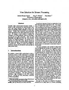
Fig. 4a (left) and 4b (right). Time moves downwards, tuples are shown as small black rectangles, and the green lines represent intra-operator dependencies. In the incorrect implementation, on the left side, the PreVwap Aggregate operator creates an output tuple (on the second vertical rail) each time four new input tuples (on the first vertical rail) have arrived to (supposedly) calculate the weighted moving average value for the stock price. Here it can be seen that an incoming tuple contributes to only one outgoing tuple, which is an indication of a problem, as this pattern is not consistent with computing a moving metric. In the corrected version, on the right side, the PreVwap Aggregate operator uses a sliding window to calculate the average value over the four last incoming tuples, thus creating an output tuple after every incoming tuple. It can be seen here that an incoming tuple contributes to four outgoing tuples (in this case, the sliding window was configured to hold four tuples at any given point in time and uses these tuples to produce the moving average).
On performing an application validation test, the developer starts by examining all operators and their interconnections, and subsequently samples the incoming and outgoing tuples in the Topology view of our tool. In principle, everything seems to look fine. To verify the behavior of the application over time, the developer now turns to the Tuple Sequence view. There the developer observes that the data flow going through the PreVwap Aggregate operator exhibits the pattern shown in Figure 4a.
From this pattern, it appears that this operator consumes four new input tuples before it produces an output tuple. However, the original application specification required that an output tuple be created with the weighted average of the last four tuples, after every new incoming tuple arrives at the operator. Clearly, the PreVwap Aggregate has been incorrectly deployed with a “tumbling window” parameter (i.e., the window state is reset every time an aggregation is produced), while the specification demanded a “sliding window” average (i.e., the window state is updated on arrival of new tuples, by discarding older ones). From an application design standpoint, using a sliding window in this operator allows for a smoother function constantly indicating the fair value prices for each stock symbol. After redeploying the application with the corrected parameter in the configuration of the Aggregate operator, the developer can observe the new (and now compliant) behavior depicted by Figure 4b. As can be seen, about four times as many output tuples are now created in the same time span. 6.3 Tracking Down the Locus of a Calculation Error Figure 5 shows the content of a tuple at the sink operator. A tuple with a positive index field, like the one shown here, indicates a trading bargain and the specific value indicates the magnitude of the bargain for ranking purposes (i.e., a bigger bargain should be acted on first, due to its higher profit making prospect).
Fig. 5. Hovering over one of the result tuples shows an (incorrect) tuple with an ask price higher than the fair price (VWAP).
However, the tuple shown in this figure as well as other tuples seen at the input port suggest that the system has spotted bargains, although, surprisingly, the ask price seems to be higher than the VWAP or fair price value predicted by the pricing model, opposite to what the definition of a bargain is. This is a clear sign that something went wrong, leaving the question of where the problem actually originated. In order to retrieve the lineage of this incorrect result, a developer can click on one of the tuples with incorrect results. This will highlight all the tuples, upstream in the application, whose contents might have impacted the outcome of the selected tuple. Moving to the left, from the tuple with the incorrect values, the developer can quickly spot the contributing tuples at the join operator. Both the fair value tuple (received from the Vwap operator and used for this computation) as well as the quote tuple (received from the QuoteFilter operator) turn out to be correct. This leads the developer to take a closer look at the BargainIndex operator. Examining the SPADE
code2 then leads to the discovery of a “greater than” sign that should have been a “less than” sign.
Fig. 6. Selecting the tuple with the incorrect value in the result operator on the right highlights its lineage, showing the upstream tuples potentially contributing to the error.
6.4 Investigating the Absence of a Result The incorrect behavior in an application sometimes manifests itself by the absence of an expected result. For example, automated unit tests set in place to ensure an application gets validated before deployment are typically built with pre-determined inputs that will lead to an expected output. Finding out why we did not observe an outcome is often more difficult than investigating an incorrect outcome. In the following debugging scenario, a developer observes that no tuples are received at the sink, as shown in Figure 7. However, the same figure also shows that all operators in front of the sink operator did receive tuples.
Fig. 7. The sink operator, to the right, does not receive any tuples (as seen by the absence of a tuple log widget). Nevertheless, tuples are arriving at preceding operators, but none are produced by the output port of the join operator. Hovering the tooltip over one of the input queues in the join operator reveals the ticker symbols for the tuples that have been received so far.
The first suspicion is that there is a problem in the BargainIndex join operator. Examining a few individual tuples at both inputs of the BargainIndex reveals that the lower port seems to receive only tuples with the ticker symbol “IBM” (shown by the 2
System S provides an integrated environment that allows developers to conveniently jump from the dataflow graph representation to the specific segment of source code implementing that segment and vice-versa [3, 5].
tooltip in the Figure 7), whereas the upper port seems to receive only tuples with a ticker symbol “LLY” (not shown). This suggests that the join operator works correctly, but simply did not find tuples with matching ticker symbols, required to evaluate and potentially indicate the existence of a bargain. The next step is to go upstream and look at the distribution of ticker symbols in the tuples flowing through the application. The visualization tool can color the tuples according to the content of an attribute belonging to the schema that defines a stream and its tuples, at the request of the user. For example, Figure 8 shows the tuples flowing through the operators in this application colored by the content of the “ticker” attribute. Each value for the ticker attribute is automatically hashed into a color. The figure shows that tuples with ticker symbol “LLY” are rendered in red, whereas tuples containing “IBM” are rendered in blue. It also reveals that the TradeFilter operator (second from the left) only forwards LLY tuples and that the QuoteFilter operator (at the bottom) only forwards IBM tuples. The solution for this problem was to change the parameterization of the TradeFilter operator, so that it also forwards IBM tuples. In this case, the problem stemmed from an (incorrectly implemented) effort at parallelizing the application [17]. Specifically, the filter condition in the Trade part of the graph was not the same as the condition in the Quote part of the graph. With this parallelization approach, the space of stock ticker symbols (around 3,000, for the New York Stock Exchange) was partitioned into ranges (e.g., from A to AAPL, from C to CIG, etc) so that replicas of the bargain discovery segment could operate on different input data concurrently, yielding additional parallelism and allowing the application to process data at a much higher rate.
Fig. 8. Tuples are colored by the ticker attribute: tuples containing “LLY” are rendered in red, “IBM” tuples are (appropriately) in blue. The TradeFilter only forwards “LLY” tuples, the QuoteFilter only allows “IBM” tuples, preventing the join operator to make matches.
6.5 Latency Analysis Understanding latency is a key challenge in streaming applications, in particular, for those that have rigid performance requirements, as is the case, for example, of many financial engineering applications. To assess latency, we must first establish what the latency metrics represent. Latency can be defined in many different ways, depending on the particular path of interest within the flow graph as well as the set of tuples involved. Second, manually capturing latency via application-level time-stamps imposes a heavy burden on the developer and often complicates the application logic. As a result, system and tooling support for analyzing latency are a critical requirement for stream processing systems. This requirement addresses the need for providing
comprehensive application understanding, especially from the perspective of userfriendly performance analysis. As an example, consider the Bargain Discovery application, discussed earlier, and the following measures of latency that are relevant to application understanding: A. Given a tuple that indicates that a bargain has been spotted, the time between (i) the arrival of the quote tuple that triggered the spotting of that new bargain and (ii) the generation of the bargain tuple itself is one of the latency metrics of interest. This latency measure helps in understanding how quickly the bargains are spotted based on the arrival of new quotes. B. Given a tuple representing a volume weighted average price (VWAP), the time between (i) the arrival of the trade tuple that triggered the price and (ii) the generation of the VWAP tuple itself is another latency metric of interest. This latency measure helps in understanding how quickly new trades are reflected in the current VWAP fair value price, which impacts the freshness of the pricing model and in turn the accuracy of the discovery (or not) of the bargains. C. Given a tuple representing a trade, the time between (i) the arrival of the trade tuple itself and (ii) the generation of the last bargain tuple that was impacted by the trade tuple in question is another latency metric of interest. This latency measure helps in understanding the duration of the impact of given trade tuple to the pricing model. It is interesting to note that the above listed use cases can be broadly divided into two categories. These categories are determined by the anchor tuple used for defining the latency, which impacts the type of workflow involved in the visual analysis of the latency. We name these categories as result-anchored and source-anchored latencies. A result-anchored latency is defined using the downstream result tuple as an anchor. It is visually analyzed by first locating the result tuple and then using the result tuple’s provenance to locate the source tuple. Use cases A and B above fall into this category, as illustrated by Figure 9, produced by our visualization tool.
Fig. 9. Visualization of the result-anchored latencies from the use cases A and B, showing the provenance of a bargain tuple and the start and end points for the computation of the resultanchored latencies.
In this figure, we mark the source tuples using a diamond shape and the result tuples using a square shape. For use cases A and B, we first locate the result tuple and use it as an anchor point to take the provenance. For use case A, the bargain tuple is our anchor point, whereas for use case B, the VWAP tuple is our anchor point. We then locate the source tuple in the lineage of the result tuple. For use case A, the
source tuple is the quote tuple, whereas for use case B, the source tuple is the last trade tuple that is in the lineage of the result tuple. Once the source and target tuples are located, the latency can be retrieved easily. A source-anchored latency is defined using the upstream source tuple as the anchor. It can be visually analyzed by first locating the source tuple and then using the source tuple’s downstream lineage to locate the result tuple. Use case C above falls into this category, as illustrated by the Figure 10.
Fig. 10. Visualization of the source-anchored latency from the use case C, showing a downstream lineage of a trade tuple and the start and end points for the computation of the source-anchored latency.
For use case C, we first locate the source tuple and use it as an anchor point to take the downstream lineage. The trade tuple is our anchor point in this case. We then locate the target tuple in the lineage of the source tuple. In this case, the result tuple of interest is the last bargain tuple produced downstream that is in the lineage of the source tuple. Once the source and target tuples are located, the latency can be retrieved easily. Finally, it should be pointed out that the average latencies and outliers can also be of interest, rather than the instantaneous latencies of specific tuples. Given that our tool has access to various samples for a given type of provenance or lineage, simple pattern analyses techniques can be used to compute average values as well as outliers for the desired latencies. For instance, the latency defined in use case A can be averaged over all the bargain tuples in the history to compute an average value. While our tool does not provide this capability yet, this represents a simple and straightforward extension.
7 Design and Implementation The System S runtime was enhanced to track inter-tuple dependencies by intercepting tuples as they leave output ports and assigning them unique tuple identifiers. These identifiers enable the receiver of a tuple to learn about the immediate origin of the tuple. To track intra-tuple dependencies, a provenance tag is added to each tuple. The provenance tag is maintained by the System S runtime based on a lightweight API exposed to application developers for specifying dependencies of output tuples to input ones. The System S runtime maintains one-step dependency only, which captures interand intra-operator dependencies, but does not include the complete provenance information, which contributes to lowering the amount of overhead imposed by
tracing operations. The visualization tool is used to reconstruct the complete provenance information from one-step data dependency information collected from multiple operator ports. The new visualization features for debugging and data flow analysis are implemented as an Eclipse plug-in and are fully integrated into System S’ Streamsight visualization environment [3, 4]. In our current prototype we use a mix of CORBA calls and files for the two-way communication between the System S runtime and the visualization. We designed the tool so that it can process and reflect near-live information from the runtime system. In particular, the data models that contain the tuple and data dependency information can be populated incrementally. Similarly, the visual frontend is able to render the new information almost immediately.
8 Conclusion In this paper we presented a new, visual environment that allows developers to debug, understand, and fine-tune streaming applications. Traditional debugging techniques, like breakpoints, are insufficient for streaming applications because cause and effect can be situated at different locations. Development environments for message-based distributed or concurrent systems offer the developer insight by aligning the distributed events with the messages that were exchanged. However, even these techniques tend to be impractical for debugging streaming applications because of the sheer volume of data that they produce. Our new environment allows the developer to limit the tracing information to execution slices, defined in time and in space. It organizes the traced tuples based on their data dependencies. This offers a natural way for the user to navigate the distributed execution space in terms of provenance and lineage. We offer two new views to the developer. The Topology view projects the execution information, i.e. the tuples, their contents and their mutual data dependencies, on the application topology graph. The Tuple Sequence view organizes tuples by time and by operator. The combination of these two views offers a natural way for a developer to explore causal paths during problem determination, as well as to carry out performance analysis.
References 1. Turaga, D., Andrade, H., Gedik, B., Venkatramani, C., Verscheure, O., Harris, D., Cox, J., Szewczyk, W., Jones, P.: Design Principles for Developing Stream Processing Applications. Software: Practice & Experience Journal, Wiley SP&E, (2010, to appear) 2. Amini, L., Andrade, H., Bhagwan, R., Eskesen, F., King, R., Selo, P., Park, Y., and Venkatramani, C: SPC: A distributed, scalable platform for data mining, Workshop on Data Mining Standards, Services and Platforms, DMSSP, Philadelphia, PA, (2006). 3. De Pauw, W., Andrade, H.: Visualizing large-scale streaming applications. Information Visualization, vol 8, pp. 87-106, Palgrave Macmillan (2009) 4. De Pauw, W., Andrade, H., and Amini, L. 2008: Streamsight: a visualization tool for largescale streaming applications. In Proceedings of the 4th ACM Symposium on Software
Visualization (Ammersee, Germany, September 16 - 17, 2008). SoftVis '08. ACM, New York, NY,pp. 125-134 (2008) 5. Gedik, B., Andrade, H., Frenkiel, A., De Pauw, W., Pfeifer, M., Allen, P., Cohen, N., Wu, KL.: Tools and strategies for debugging distributed stream processing applications, Software: Practice & Experience, Vol. 39 , Issue 16 (2009) 6. Gedik, B., Andrade, H., Wu, K-L., Yu, P.S., Doo, M.: SPADE: The System S Declarative Stream Processing Engine. International Conference on Management of Data, ACM SIGMOD (2008) 7. Wang, H.Y., Andrade, H., Gedik, B., Wu, K-L.: A Code Generation Approach for AutoVectorization in the SPADE Compiler. International Workshop on Languages and Compilers for Parallel Computing, pp. 383-390 (2009) 8. Khandekar, R., Hildrum, K., Parekh, S., Rajan, D., Wolf, J., Andrade, H., Wu, K-L., Gedik, B.: COLA: Optimizing Stream Processing Applications Via Graph Partitioning. ACM/IFIP/USENIX International Middleware Conference, Middleware (2009) 9. Stanley, T., Close, T., Miller, M.S.: Causeway: A message-oriented distributed debugger. Technical report, HPL-2009-78, HP Laboratories (2009) 10. Vijayakumar, N., Plale, B.: Towards Low Overhead Provenance Tracking in Near RealTime Stream Filtering. In: International Provenance and Annotation Workshop, IPAW (2006) 11. Blount, M., Davis, J., Misra, A., Sow, D., Wang, M.: A Time-and-Value Centric Provenance Model and Architecture for Medical Event Streams. In: ACM HealthNet Workshop, pp. 95–100 (2007) 12. Misra, A., Blount, M., Kementsietsidis, A., Sow, D., Wang, M.: Advances and Challenges for Scalable Provenance in Stream Processing Systems. In: International Provenance and Annotation Workshop, IPAW (2006) 13. De Pauw, W., Lei, M., Pring, E., Villard, L., Arnold, M., and Morar, J.F.: Web Services Navigator: Visualizing the execution of Web Services, IBM Systems Journal, Vol. 44, No. 4 (2005) 14. De Pauw, W., Hoch, R., Huang, Y.: Discovering Conversations in Web Services Using Semantic Correlation Analysis, International Conference on Web Services 2007: pp. 639646 (2007) 15. Aguilera, M. K., Mogul, J. C., Wiener, J. L., Reynolds, P., and Muthitacharoen, A.: Performance debugging for distributed systems of black boxes, Proceedings of the Nineteenth ACM Symposium on Operating Systems Principles (Bolton Landing, NY, USA, October 19 - 22, 2003), SOSP '03, ACM, New York, NY, pp. 74-89 (2003) 16. Wong, W.E., Qi, Y.: An Execution Slice and Inter-Block Data Dependency-Based Approach for Fault Localization. In: Proceedings of the 11th Asia-Pacific Software Engineering Conference, pp. 366 - 373 (2004) 17. Andrade, H., Gedik, B., and Wu, K-L. Scale-up Strategies for Processing High-Rate Data Streams in System S. International Conference on Data Engineering, IEEE ICDE, (2009) 18. Zhang, X.J., Andrade, H., Gedik, B., King, R., Morar, J., Nathan, S., Park, Y., Pavuluri, R., Pring, E., Schnier, R., Selo, P., Spicer, M., Venkatramani, C.: Implementing a HighVolume, Low-Latency Market Data Processing System on Commodity Hardware using IBM Middleware. Workshop on High Performance Computational Finance, (2009)