56. VOL. 21, NO. 4, 2008. Visual Revelations. Howard Wainer,. Column Editor. Looking at Blood Sugar. Howard Wainer and Paul Velleman. 2010. 2000. 1990.
Visual Revelations
Howard Wainer,
Column Editor
Looking at Blood Sugar Howard Wainer and Paul Velleman
I
56
VOL. 21, NO. 4, 2008
80
Prevalence of diabetes in the U.S. (per 1000 population)
t is estimated that there are 20.8 million children and adults in the United States, or 7% of the population, with diabetes. Of these, 14.6 million have been diagnosed and 6.2 million (or nearly one-third) are unaware they have the disease (www.diabetes.org/about-diabetes.jsp). The large proportion of undiagnosed diabetics adds uncertainty to the estimates of the total number, but through the use of multiple sources and statistical adjustment, we can obtain a rough view (see Figure 1). Using adjusted estimates of the prevalence of this disorder, we can see that, throughout the past 70 years, the growth of diabetes in the United States has been exponential. There have been many causes proposed for this explosion, including increased obesity, decreased physical activity, a shift toward more processed foods, and an aging population. Though there are many other risk factors, we would like to focus on making the treatment of the disease more efficacious through improved communication of the consequences of treatment choices and behaviors. Left untreated, diabetes has many serious consequences, including—but not restricted to—liver and kidney damage and circulatory problems leading to blindness, neuropathy, and loss of limbs. Effective treatment requires close cooperation between the physician and the patient. The physician can prescribe
60
40
20
0
1930
1940
1950
1960
1970
1980
1990
2000
2010
Figure 1. Estimates of the prevalence of diabetes in the United States shown as the number per 1,000 in the population. The fitted curve is an exponential function.
• How large are the variations in blood sugar level that take place over the course of the day due to normal daily events such as eating meals, exercising, and sleeping? drugs and changes in diet and exercise regimes, but only the patient can implement those changes. Often, the patient is given both general and specific guidelines, but the effects of following or not following those guidelines can only be seen after implementation. The record of success cannot be described as an unqualified success. Indeed, as Jinan Saaddine and coauthors describe in “Improvements in Diabetes Processes of Care and Intermediate Outcomes: United States, 1988–2002,” “Despite the many improvements, two in five people with diabetes still have poor cholesterol control, one in three have poor blood pressure control, one in five have poor glucose control.” Why? Surely the consequences of not controlling cholesterol, glucose, and blood pressure are both dire and clearly understood. Just as surely, the answer to the causal “Why?” has many parts. We would like to consider just one of them here: The communication of current status to the patient is not as effective as it could be.
sugar under tight control and the role diet and exercise play in so doing. To aid the patient in controlling blood sugar, s/he is given a small device that (i) reads a small blood sample and indicates its glucose content within seconds; (ii) records the reading in (i), along with the time and date it was taken; (iii) allows the inputting of various classifying characteristics (e.g., before a meal, after a meal, or none); (iv) calculates mean blood sugar levels for the past seven days, 14 days, and 30 days; and (v) shows these averages for each of the subclassifications indicated in (iii). All in all, this small instrument is a remarkable device. As remarkable as it is, however, it could be more useful still with a few minor modifications, namely modifying how it summarizes and displays the data.
What Is
• How am I doing overall? This is a long-term question that focuses on the blood sugar levels over extended periods of time to evaluate the efficacy of the various strategies being employed to control it.
Once a patient is diagnosed with diabetes, a number of actions take place. Among them are extensive counseling about the importance of keeping blood
What Might Be Before we reconsider how to compute and display summaries of blood sugar data, let us first consider the key questions these data may help answer. By our estimation, there are three:
• Are there any unusual excursions in blood sugar? How large are they? What causes them? Each question has obvious medical implications. The first is the overall evaluation of the therapy. If the therapy has the character desired, whatever is being done is working. But, if all we find is that the mean blood sugar is too high, we have no immediate clues to aid in remediation. The second question is primarily intermediate in character. We must know how much variation is usual before we can answer the third question: What is unusual? Management of blood sugar means more than keeping its typical amount in a particular range. It also is important to keep its variation within prespecified bounds (i.e., between 80 and 140 mg/dl). The answer to this question can be both descriptive and prescriptive. If blood sugar shows unusually large variation before and after dinner, then one should consider eating less at dinner. Such a result is important, but unavailable solely from the answer to question one. The third question is of least importance to the physician, but of potentially greatest import to the patient, for large excursions from what is normal will invariably have an associated story (e.g., a large cookie, an ice cream cone, CHANCE
57
Table 1—A Sequence of Seven Blood Sugar Measurements (mg/ dl) and a Running Mean of Three Smooth of These Measurements
Blood sugar (mg/dl)
250
Blood Sugar
200
150 100
65
70
75
Residuals smooth Residualsfrom from 33smooth
Figure 2. Glucose tolerance test. Thirty-seven Days data points taken over 10 days. The smooth connecting function is a running mean every three points.
80 80 40 40 00
-40 -40
65 65
70 70
75 75
Days Days Figure 3. The residuals of the data points from the smooth curve shown in Figure 2
too much beer, or too many pretzels). Because each excursion has a specific story, it also suggests an obvious remediation: Don’t do it any more. It is the immediate, clear, and specific feedback from the answer to question (iii) that has the greatest likelihood of aiding the patient in shaping his/her behavior and thus better controlling blood sugar. In addition, as we will see, these are not independent questions. By estimating the pattern of daily variation, we should be able to obtain a more reliable estimate of long-term trends. Even an isolated large excursion can have a significant effect on both the estimated daily variation and the long-term trend when these are represented by averages. We propose simple methods to address both of these problems with the result of providing better information to both doctor and patient. What is the best way to answer these three questions and convey the answers to the patient? The current approach is a listing of numbers—either the actual 58
VOL. 21, NO. 4, 2008
readings or three different averages (e.g., 7-, 14- and 30-day averages). Neither a list of numbers nor the use of averages is the best we can do, and, in combination, they are worse still. Our approach to summarization uses resistant statistical methods, and our approach to presentation is graphical. In the latter, we join with the brothers Farquhar in their belief, written in Economic and Industrial Delusions, in the following: The graphical method has considerable superiority for the exposition of statistical facts over the tabular. A heavy bank of figures is grievously wearisome to the eye, and the popular mind is as incapable of drawing any useful lessons from it as of extracting sunbeams from cucumbers. What is a resistant method? In short, it is a method not affected by a few unusual points. A median is resistant; a mean is not.
Smooth
104
•
117
110.7
111
114.3
115
116.3
123
116.7
112
117.3
117
101.7
Why resistant? The current method of summarizing blood sugar results is taking averages. An average is fine for some things, but because it uses all the information equally, it has some weaknesses. The idea of a summary is that it essentially says “This is typical of the data, most of them lie nearby.” The arithmetic mean satisfies this heuristic when the data follow a bell-shaped curve. But, it does not follow it when there are only a few very unusual points. For example, consider the following blood sugar readings: 90, 93, 95, 102, 210 The mean is 118. Thus, the average is not in the middle of the data, nor is it near any of the readings. In fact, if we subtract the mean from each reading, we get a vector of residuals: -28, -25, -23, -16, 82 Using the mean as the summary statistic has had two unfortunate results. First, it located the middle, where there were no scores nearby. Second, it distributed the mislocation among all the observations. A better characterization would have told us that most of the scores were near 95, but one was very far away at 210. That latter piece is of critical importance, for it is by having that one outlying observation pointed out that the patient can then look for a cause. If a probable cause can be identified, the patient can modify his or her behavior in hopes of avoiding similar excursions in the future. A much more resistant alternative to the mean is the median, 95. The
Smoothing When we have data arranged over time, it is often helpful to find a smooth trace through an otherwise scattered or choppy plot of the data. A smooth trace can show the overall pattern, free of the ‘noise’ of point-to-point variation. And—often more important—it can provide a central summary from which to notice isolated exceptions to the overall pattern. A smooth trace through a sequence of values serves much the same function as a summary of the middle of a single batch of values: It provides a central summary and facilitates identifying exceptions. And, for reasons that will be clear presently, smooth traces can suffer from the same sensitivity to isolated excursions as we saw with the mean. One common way to find a smooth trace is to take local averages of values in the sequence. The result is called a running mean, or sometimes a moving average. For example, Table 1 shows a sequence of blood sugar measurements and a running mean of three of these measurements. The first smooth value, 110.7, is found as the mean of 104, 117, and 111. But running means suffer from the same sensitivity to outlying values as we saw for means. Figure 2 shows a sequence of blood sugar measurements with a single outlying value (due to a glucose tolerance test) and the smooth found by running means of three.
260 260 240 240
200 200 180 180
160 160
Diagnosed as diabetic
Blood sugar (mg/dl)
220 220
Blood Sugar (mg/dl)
residuals are then -5, -2, 0, 7, 115, leaving no doubt which observation is the extreme outlier. The median and mean are the extremes of a continuum of summaries of the middle. Although the mean averages all the values, the median classifies them only as “big” and “small” to pick out the middle one. A measure intermediate in its calculation between the median and the mean is the trimmed mean, which symmetrically lops off some the largest and smallest values and averages those middle ones that remain. By adjusting the percentage of values trimmed off, we can ‘tune’ a trimmed mean to be like the median (by trimming just less than 50%) or like the mean (by trimming very few). In our toy example, a 20% trimmed mean would trim off the largest (210) and smallest (90) values and average the three remaining ones to obtain 96.67.
140 140
120 120 100 100 80 80 1990 1990
1995 1995
2000 2000
2005 2005
2010 2010
Figure 4. Fifteen years of fasting blood sugar tests showing both a pre-diabetic condition indicated by steady increases and the obvious onset of diabetes in 2006
The data points are measured blood sugar levels. The connecting curve represents the smooth values. Note the contamination of three smooth values by a single outlying value. If we used a larger smoothing window, say a running mean every five points instead of three, the excursion caused by the one outlying point would be smaller, but more points would be affected. Because each smooth value averages three data values, the extreme value contaminates three of the values in the smooth trace. What may be of greater concern is that the residuals— the difference between the data and the smooth—are also contaminated. It is the residuals a patient would look at to be alerted to a deviation from the overall trend that might require attention. But, as Figure 3 shows, this approach could raise false alarms. When looking at the residuals from a running average of successive sets of three blood sugar levels, if one original value is unusually high, the residuals show the spike, but also suggest two blood sugar levels that only appear to be low because the spike has contaminated their smooth values. The solution is to use a resistant smoothing method. Smoothers can be based on running medians or running trimmed means. Resistant smoothers often give a less smooth trace, so special methods (beyond the scope of this article) can be use to improve the smoothness of the trace.
An Example The subject is a 63-year-old male in generally good health. He is 6’4” and weighed 230 pounds at the time of diagnosis. He exercises robustly five days a week, and has done so for his entire adult life. Shown in Figure 4 is a plot of his fasting blood sugar taken over the past 15 years. From 1992 until 2005, it was under 140 mg/dl, but, even in 2005, was trending upward portending a prediabetic condition. In 2006, the annual result increased profoundly to 183 and the patient was told to lose five pounds and come back in six months. Six months later, the patient returned 10 pounds lighter with fasting blood sugar of 249. He was diagnosed at that point as a type 2 diabetic and the following corrective actions were taken: • A one-gram-a-day dosage of Metformin was prescribed and then titrated up to two grams a day over a two-week period. • The patient limited his food intake to 2,700 calories a day—divided into 40% carbohydrates, 30% fats, and 30% proteins—and the caloric intake was spread more evenly across the day. • Exercise was increased from an hour to 90 minutes a day • He was given a blood sugar sensing meter and began to check glucose levels four to five times a day. CHANCE
59
250 250
BloodSugar sugar (mg/dl) Blood (mg/dl)
200 200
150 150
100 100
50 50
0
10 10
20 20
30 30
40
50 50
60 60
Day Day
15
5
5
-5
-5
-15
-15
-35
0
5
Lunch
Exercise
-25
Noon
10
15
Snack
15
Dinner
25
Breakfast
25
20
Hourly blood sugar effects (mg/dl)
Hourly blood sugar effects (mg/dl)
Figure 5. Taken over two months, 215 blood sugar readings beginning at diagnosis. Superimposed over the readings is a curve indicating the outcome of the treatments being used to control blood sugar. Blood sugar levels declined after treatment began and seem near asymptote after the first month.
-25
24
-35
Time of day
Figure 6. The blood sugar readings collapsed over days and summarized to show the typical daily variation. The plot is annotated to explain the variations. Data from March 8 until April 23, 2007.
The readings, taken using the device described earlier in this article over a period of two months, are displayed in three plots. The first, shown in Figure 5, reflects all the readings shown sequentially with a resistantly smoothed curve superimposed over them. It shows a steep decline of typical blood sugar as treatment began with a leveling off after the first month. We also note that the variation around the plotted curve continues to diminish beyond the initial month. 60
VOL. 21, NO. 4, 2008
The decline in blood sugar has four plausible causes: medication, change in diet, change in exercise, and the patient’s loss of 25 more pounds. Because all these possible causes took place simultaneously, we cannot partition the improvement in blood sugar levels among these four changes. While we can see the variation across days, and roughly within each day, the within-day variation is more obvious if we make a plot that has the 24 hours of the day on the horizontal axis and the
hourly blood sugar effects on the vertical. Blood sugar effects, in this instance, are what result after we subtract the resistant curve in Figure 5 from the actual blood sugar levels—thus what we plot has been adjusted for the long-term trend. We then aggregate across days and fit a resistant curve. Such a plot is shown as Figure 6. The curve shown in Figure 6 indicates clearly that the typical range of variation over the course of a day is about 40 mg/ dl. We see obvious spikes after each meal and a big drop when blood sugar is measured after noon-time exercise. The third descriptive plot is of the residuals. This is a plot of blood sugar levels after removing the long-term trend effects shown in Figure 5 and the daily effects shown in Figure 6. What remains are the unusual changes in blood sugar not accounted for by those other two effects. The residual plot is shown as Figure 7. One can easily see how it is the most immediately useful diagnostic plot for the patient. Each large residual should have a story associated with it. We have indicated just a few. We note that most large residuals occurred early in treatment before the patient’s blood sugar had stabilized. The unusually low readings were invariably due to exercise. The two large positive residuals that occurred more than two weeks after diagnosis were due to specific eating events. This plot makes it clear that these are to be avoided in the future.
How Were the Data Summarized? The underlying ideas behind robust smoothing are not strictly based on some form of mathematical optimization. They are meant to be far more rough-and-ready than that, although the sweetness of elegance lingers on. Hence, many alternative approaches will serve well. The one that we have used here was developed by John Tukey in a preliminary edition of his now classic Exploratory Data Analysis and dubbed by him “53h twice.” This odd title is completely descriptive. The original ordered data are smoothed by taking running medians every five (the 5 in 53h). Next, these medians are smoothed by taking running medians every three (the 3 in 53h). Next, these twice-smoothed values are “hanned,” which means they too are smoothed three at a time with a weighted linear combination (smoothed value of
Last, it seems sensible to discuss implementation of this approach. The current blood meters are wondrous devices that have in their innards the hardware necessary to implement our methods. They have plenty of storage, and even if they didn’t, adding more would be very cheap. Their screens can show statistical graphs as easily as they now show letters and other icons. To boost their capabilities in the ways we suggest, they want only some programming.
Blood sugar residuals (mg/dl)
Blood Sugar Residuals (mg/dl)
100 100 80 80
Indian Indian restaurant Restaurant
60 60
Pretzel Pretzel
40 40 20 20 00 -20 -20 -40 -40
Further Reading
Extra exercise exercise Extra
-60 -60
Farquhar, A.B. and Farquhar, H. (1891) Economic and Industrial Delusions. New York: G. P. Putnam’s Sons.
-80 -80 -100 -100 0 0
10 10
20 20
30 30
40 40
50 50
60 60
70 70
Day
Figure 7. A plot of the residuals in blood sugar readings after subtracting the long-term trend and daily variation. Some unusual points are annotated to indicate probable cause.
x(i) = [x(i-1) + 2x(i) + x(i+1)]/4). This yields an initial smoothing, which is then subtracted from the original values and the residuals are calculated. Next, the residuals are smoothed by 53h again. The sum of the two smooths is the final smooth. Then, the final smooth is subtracted from the original data to yield the residuals. Tukey was fond of describing the final result as an equation in which the data = smooth + rough. The smooth is the result of 53h twice, and the rough is the vector of residuals. Less arcane methods may work just as well, but for reasons of trust—borne of prior use— and sentiment, we chose this one. This method is what yielded the smooth shown in Figure 5. The residuals from the first smooth were then ordered by time of day, collapsing over days, and smoothed again using 53h twice. The resulting smooth was shown as Figure 6. Residuals from this smooth were then ordered by date and shown as Figure 7. Large residuals, in either direction, were interpreted.
Conclusions Diabetes is a dangerous disease that is spreading quickly. To be fully effective, its treatment requires the full participation of the patient. Moreover, it typically requires the patient to lose weight and exercise regularly—two things that are difficult to do for most people. It is our
contention that providing immediate and easily understood feedback on the relationship between the patient’s diet and exercise on blood sugar will help to reinforce proper behavior. We suggest that the use of average blood sugar has flaws that are easily ameliorated through the use of resistant/robust methods such as the one we have described here. In addition, by providing the results in a graphic form, the feedback is more vivid. Note that the word “graphic” in ordinary speech means “literal lifelikeness,” but when used to describe an iconic visual display of data, its meaning is almost exactly the opposite. We also contend that by partitioning the blood sugar results into three pieces, we highlight information that both clinician and patient need. Specifically, the overall trend curve illustrated in Figure 5 provides a clear and accurate summary of the efficacy of the treatment vis-à-vis blood sugar. At the same time, the residual plot illustrated in Figure 7 allows the patient to see immediately the extent to which a specific action on his/her part has affected blood sugar, hence implicitly suggesting changes in future behavior. The depiction of residuals from a resistant smooth makes explicit how important is the accurate recording of the details of eating and exercise, for only through careful records can the stories of the residuals be told and acted upon.
Saaddine, B., Cadwell, B., Gregg, E., Engelglau, M., Vinicor, F., Imperatore, G., and Narayan, V. (2006) “Improvements in Diabetes Processes of Care and Intermediate Outcomes: United States, 1988–2002.” Annals of Internal Medicine, 465. Available for download at www.cdc.gov/diabetes/news/ docs/diabetescare.htm. Tukey, J.W. (1977) Exploratory Data Analysis. Reading, MA: AddisonWesley. Data sources for Figure 1 Early release of 2006 data in Chapter 14 of the National Health Interview Survey, prepared under the auspices of the Centers for Disease Control and prevention. Available at www.cdc.gov/nchs/data/nhis/earlyrelease/ earlyrelease200703.pdf. Kenny, S.J., Aubert, R.E., and Geiss, L.S. (1994) Prevalence and Incidence of Non-Insulin-Dependent Diabetes. Chapter 4 in Diabetes in America (2nd ed.). (http://diabetes.niddk.nih.gov/dm/ pubs/america). LaPorte, R.E., Matsushima, M., and Chang, Y-F. (1994) Prevalence and Incidence of Insulin-Dependent Diabetes. Chapter 3 in Diabetes in America (2nd ed.). (http://diabetes.niddk.nih.gov/ dm/pubs/america)
Column Editor: Howard Wainer, Distinguished Research Scientist, National Board of Medical Examiners, 3750 Market Street, Philadelphia, PA 19104; hwainer@ nbme.org CHANCE
61