SUBMITTED TO IEEE TVCG SPECIAL ISSUE ON VISUAL ANALYTICS
1
Visual Signatures in Video Visualization Min Chen, Ralf P. Botchen, Rudy R. Hashim, Daniel Weiskopf Member, IEEE, Thomas Ertl Member, IEEE, and Ian Thornton
Abstract— Video visualization is a computation process that extracts meaningful information from original video data sets and conveys the extracted information to users in appropriate visual representations. This paper presents a broad treatment of the subject, following a typical research pipeline involving concept formulation, system development, a path-finding user study and a field trial with real application data. In particular, we have conducted a fundamental study on the visualization of motion events in videos. We have, for the first time, deployed flow visualization techniques in video visualization. We have compared the effectiveness of several different abstract visual representations of videos. We have conducted a user study to examine whether users are able to learn to recognize visual signatures of motions, and to assist in the evaluation of different visualization techniques. We have applied our understanding and the developed techniques to a set of application video clips. Our study has demonstrated that video visualization is both technically feasible and cost-effective. It provided the first set of evidence confirming that ordinary users can accustom to the visual features depicted in video visualizations, and can learn, without much effort, to recognize visual signatures of a variety of motion events. Index Terms— video visualization, volume visualization, flow visualization, human factors, user study, visual signatures, video processing, optical flow, GPU-rendering.
I. I NTRODUCTION
A
video is a piece of ordered sequential data, and viewing videos is a time-consuming and resourceconsuming process. Video visualization is a computation process that extracts meaningful information from original video data sets and conveys the extracted information
M. Chen and R. R. Hashim are with Department of Computer Science, University of Wales Swansea, Singleton Park, Swansea SA2 8PP, UK. Email: {m.chen,csrudy}@swansea.ac.uk. R. Botchen and T. Ertl are with Visualization and Interactive Systems Group, University of Stuttgart, Universitaetsstr. 38, D70569 Stuttgart, Germany. Email: {botchen,thomas.ertl}@vis.unistuttgart.de. D. Weiskopf is with School of Computer Science, Simon Fraser University, Burnaby, BC V5A 1S6, Canada. Email:
[email protected]. I. Thornton is with Department of Psychology, University of Wales Swansea, Singleton Park, Swansea SA2 8PP, UK. Email:
[email protected].
to users in appropriate visual representations. The ultimate challenge of video visualization is to provide users with a means to obtain a sufficient amount of meaningful information from one or a few static visualizations of a video using O(1) amount of time, instead of viewing the video using O(n) amount of time where n is the length of the video. In other words, can we see time without using time? In many ways, video visualization fits the classical definition of visual analytics [27]. For example, conceptually it bears some resemblance to notions in mathematical analysis. It can be considered as an ‘integral’ function for summarizing a sequence of images into a single image. It can be considered as a ‘differential’ function for conveying the changes in a video. It can be considered as an ‘analytic’ function for computing temporal information geometrically. Video data is a type of 3D volume data. Similar to the visualization of 3D data sets in many applications, one can construct a visual representation by selectively extracting meaningful information from a video volume and projecting it onto a 2D view plane. However, in many traditional applications (e.g., medical visualization), the users are normally familiar with the 3D objects (e.g., bones or organs) depicted in a visual representation. In contrast with such applications, human observers are not familiar with the 3D geometrical objects depicted in a visual representation of a video because one spatial dimension of these objects is in fact the temporal dimension. The problem is further complicated by the fact that, in most videos, each 2D frame is the projective view of a 3D scene. Hence, a visual representation of a video on a computer display in effect is a 2D projective view of a 4D spatiotemporal domain. Depicting temporal information in a spatial geometric form (e.g., a graph showing the weight change of a person over a period) is an abstract visual representation of a temporal function. We therefore call the projective view of a video volume an abstract visual representation of a video, which is also a temporal function. Considering that the effectiveness of abstract representations, such as a temporal weight graph, has been shown in many applications, it is more than instinctively plausible to explore the usefulness of video visualization, for
SUBMITTED TO IEEE TVCG SPECIAL ISSUE ON VISUAL ANALYTICS
which Daniel and Chen proposed the following three hypotheses [6]: 1) Video visualization is an (i) intuitive and (ii) costeffective means of processing large volumes of video data. 2) Well constructed visualizations of a video are able to show information that numerical and statistical indicators (and their conventional diagrammatic illustrations) cannot. 3) Users can accustom to visual features depicted in video visualizations, or can be trained to recognize specific features. The main aim of this work is to evaluate these three hypotheses, with a focus on the visualization of motion events in videos. Our contributions include: •
•
•
•
•
We have, for the first time, considered the video visualization as a flow visualization problem, in addition to a volume visualization. We have developed a technical framework for constructing scalar and vector fields from a video, and for synthesizing abstract visual representations using both volume and flow visualization techniques. We have introduced the notion of visual signature for symbolizing abstract visual features that depict individual objects and motion events. We have focused our algorithmic development and user study on the effectiveness of conveying and recognizing visual signatures of motion events in videos. We have compared the effectiveness of several different abstract visual representations of motion events, including solid and boundary representations of extracted objects, difference volumes, motion flows depicted using glyphs and streamlines. We have conducted a user study, resulting in the first set of evidence for supporting hypothesis (3). In addition, the study has provided an interesting collection of findings that can help us understand the process of visualizing motion events through their abstract visual representations. We have applied our understanding and the developed techniques to a set of real videos collected as benchmarking problems in a recent computer vision project [10]. This has provided further evidence to support hypotheses (1) and (2). II. R ELATED W ORK
Although video visualization was first introduced as a new technique and application of volume visualization [6], it in fact reaches out to a number of other disciplines. The work presented in this paper relates to video
2
processing, volume visualization, flow visualization and human factors in visualization and motion perception. Automatic video processing is a research area residing between two closely related disciplines, image processing and computer vision. Many researchers studied video processing in the context of video surveillance (e.g., [4], [5]), and video segmentation (e.g., [19], [25]). While such research and development is no doubt hugely important to many applications, the existing techniques for automatic video processing are normally applicationspecific, and are generally difficult to adapt themselves to different situations without costly calibration. The work presented in this paper takes a different approach from automatic video processing. As outlined in [27], it is intended to ‘take advantage the human eye’s broad bandwidth pathway into the mind to allow users to see, explore, and understand large amounts of information at once’, and to ‘convert conflicting and dynamic data in ways that support visualization and analysis’. A number of researchers noticed the structural similarity between video data and volume data commonly seen in medical imaging and scientific computation, and have explored the avenue of applying volume rendering techniques to solid video volumes in the context of visual arts [12], [16]. Daniel and Chen [6] approached the problem from the perspective of visualization, and demonstrated that video visualization is potentially an intuitive and cost-effective means of processing large volumes of video data. Flow visualization methods have a long tradition in scientific visualization [17], [21], [31]. There exist several different strategies to display the vector field associated with a flow. One approach used in this paper relies on glyphs to show the direction of a vector field at a collection of sample positions. Typically, arrows are employed to encode direction visually, leading to hedgehog visualizations [15], [8]. Another approach is based on the characteristic lines, such as streamlines, obtained by particle tracing. A major problem of 3D flow visualization is the potential loss of visual information due to mutual occlusion. This problem can be addressed by improving the perception of streamline structures [14] or by appropriate seeding [11]. In humans, just as in machines, visual information is processed by capacity and resource limited systems. Limitations exist both in space (i.e., the number of items to which we can attend) [22], [28] and in time (i.e., how quickly we can disengage from one item to process another) [20], [23]. Several recent lines of research have shown that in dealing with complex dynamic stimuli these limitations can be particularly problematic [3]. For
SUBMITTED TO IEEE TVCG SPECIAL ISSUE ON VISUAL ANALYTICS
example, the phenomena of change blindness [24] andinattentional blindness [18] both show that relatively large visual events can go completely unreported if attention is misdirected or overloaded. In any application where multiple sources of information must be monitored or arrays of complex displays interpreted, the additional load associated with motion or change (i.e. the need to integrate information over time) could greatly increase overall task difficulty. Visualization techniques that can reduce temporal load, clearly have important human factors implications. III. C ONCEPTS
AND
OF
(a) five frames (No.: 0, 5, 10, 15, 20) selected from a video
D EFINITIONS
A video, V, is an ordered set of 2D image frames, {I1 , I2 , . . . , In }. It is 3D spatiotemporal data set, usually resulting from a discrete sampling process such as filming and animation. The main perceptive difference between viewing a still image and a video is that we are able to observe objects in motion (and stationary objects) in an video. For the purpose of maintaining the generality of our formal definitions, we include motionlessness as a type of motion in the following discussions. Let m be a spatiotemporal entity, which is an abstract structure of an object in motion, and encompasses the changes of a variety of attributes of the object including its shape, intensity, color, texture, position in each image, and relationship with other objects. Hence the ideal abstraction of a video V is to transform it to a collection of representations of such entities {m1 , m2 , . . . , }. Video visualization is thereby a function, F : V → I, that maps a video V to an image I, where F is normally realized by a computational process, and the mapping involves the extraction of meaningful information from V and the creation of a visualization image I as an abstract visual representation of V. The ultimate scientific aim of video visualization is to find functions that can create effective visualization images, from which users can recognize different spatiotemporal entities {m 1 , m2 , . . . , } ‘at once’. A visual signature, V (m), is a group of abstract visual features related to a spatiotemporal entity m in a visualization image I, such that users can identify the object, the motion or both by recognizing V (m) in I. In many ways, it is notionally similar to a handwritten signature or a signature tune in music. It may not necessarily be unique and it may appear in different forms and different context. Its recognition depends on the quality of the signature as well as the user’s knowledge and experience. IV. T YPES
3
V ISUAL S IGNATURES
Given a spatiotemporal entity m (i.e., an object in motion), we can construct different visual signatures
(b) a visual hull
(c) an object boundary
(d) a difference iamge
(e) a motion flow
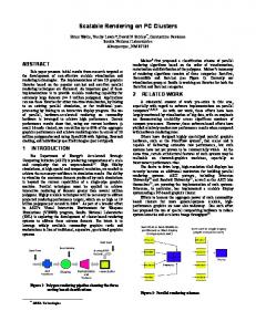
Fig. 1. Selected frames of a simple up-and-down motion, depicting the first of the five cycles of the motion, together with examples of its attributes associated with frame 1.
to highlight different attributes of m. As mentioned in Section III, m encompasses the changes of a variety of attributes of the object. In this work, we focus on the following time-varying attributes: • the shape of the object, • the position of the object, • the object appearance (e.g., intensity and texture), • the velocity of the motion. Consider a 101-frame animation video of a simple object in a relatively simple motion. As shown in Figure 1(a), the main spatiotemporal entity contained in the video is a textured sphere moving upwards and downwards in a periodic manner. To obtain the time-varying attributes about the shape and position of the object concerned, we can extract the visual hull of the object in each frame from the background scene. We can also identify the boundary of the visual hull, which to a certain extent conveys the relationship between the object and the its surroundings (in this simple case, only the background). Figures 1(b) and (c) shows the solid and boundary representations of a visual hull. To characterize the changes of the object
SUBMITTED TO IEEE TVCG SPECIAL ISSUE ON VISUAL ANALYTICS
appearance, we can compute the difference between two consecutive frames, and Figure 1(d) gives an example difference image. We can also establish a 2D motion field to describe the movement of the object between each pair of consecutive frames, as shown in Figure 1(e). There is very large collection of algorithms for obtaining such attributes in the literature, and we will describe our algorithmic implementation in Section VI. Compiling all visual hull images into a single volume results in a 3D scalar field, which we call extracted object volume. Similarly, we obtain an object boundary volume and a difference volume which are also in the form of 3D scalar fields. The compilation of all 2D motion fields in a single volumetric structure gives us a motion flow into the form of a 3D vector field. Given these attribute fields of the spatiotemporal entity m, we can now consider the creation of different visual signatures for m. One can find numerous ways to visualize such scalar and vector fields individually or in a combinational manner. Without over-complicating the user study to be discussed in Section V, we selected four types of visualization for representing visual signatures. Each type of visual signature highlights certain attributes of the object in motion, and reflects a strength of a particular volume or flow visualization technique. All four types of visualization can be synthesized in real time, for which we will give further technical details in Section VI. We also chose the horseshoe view [6] as the primary view representation. Despite that it has an obvious shortcoming (i.e., the x-axis on the right part of the visualization points to the opposite direction of that on the left), we cannot resist its enticing merits as follows: • It maximizes the use of a rectangular display area typically available in a user interface. • It places four faces of a volume, including the starting and finishing frames, in a front view. • It conveys the temporal dimension differently from the two spatial dimensions. . Since our user study (Section V) did not involve the human factors for identifying a specific direction from a visual signature, on the whole the horseshoe view served the objectives of the user study better than other view presentations. A. Type A: Temporal Visual Hull This type of visual signature displays a projective view of the temporal visual hull of the object in motion. Steady features, such as background, are filtered away. Figure 2(a) shows a horseshoe view of the extracted object volume for the video in Figure 1. The temporal visual hull, which is displayed as an opaque object, can be seen wiggling up and down in a periodic manner.
4
(a) Type A: temporal visual hull
(b) Type B: 4-band difference volume
(c) Type C: motion flow with glyphs
(d) Type D: motion flow with streamlines Fig. 2. Four types of visual signatures of an up-and-down periodic motion given in Figure 1.
B. Type B: 4-Band Difference Volume Difference volumes played an important role in [6], where amorphous visual features rendered using volume raycasting successfully depicted some motion events in their application examples. However, their use of transfer functions encoded very limited semantic meaning. For
SUBMITTED TO IEEE TVCG SPECIAL ISSUE ON VISUAL ANALYTICS
this work, we designed a special transfer function that highlights the motion and the change of a visual hull, while using a relatively smaller amount of bandwidth to convey the change of object appearance (i.e., intensity and texture). Consider two example frames and their corresponding visual hulls, Oa and Ob in Figures 3(a) and (b), we classify pixels in the difference volume to be computed into four groups as shown in 3(c), namely (i) background (6∈ Oa ∧ 6∈ Ob ), (ii) new pixels (6∈ Oa ∧ ∈ Ob ), (iii) disappearing pixels (∈ Oa ∧ 6∈ Ob ), and (iv) overlapping pixels (∈ Oa ∧ ∈ Ob ). The actual difference value of each pixel, which typically results from a change detection filter, is mapped to one of four bands according to the group that the pixel belongs to. This enables the design of a transfer function that encodes some semantics in relation to the motion and geometric change. For example, Figure 2(b) was rendered using the transfer function illustrated in Figure 3(d), which highlights new pixels in nearly-opaque red and disappearing pixels in nearly-opaque blue, while displaying overlapping pixels in translucent grey and leaving background pixels totally transparent. Such a visual signature gives a clear impression that the object is in motion, and to a certain degree, provides some visual cues of velocity.
5
visualizing the motion flow field associated with a video. This type of visual signature combines the boundary representation of a temporal visual hull with arrow glyphs showing the direction of motion at individual volumetric positions. It is necessary to determine an appropriate density of arrows, as too many would clutter a visual signature, or too few would lead to substantial information loss. We thereby used a combination of parameters to control the density of arrows, which will be detailed in Section VI. Figure 2(c) shows a Type C visual signature of a sphere in an up-and-down motion. In this particular visualization, colors of arrows were chosen randomly to enhance the depth cue of partially occluded arrows. Note that there is a major difference between the motion flow field of a video and typical 3D vector fields considered in flow visualization. In a motion flow field, each vector has two spatial components and one temporal component. The temporal component is normally set to a constant for all vectors. We experimented with a range of different constants for the temporal component, and found that a non-zero constant would confuse the visual perception of the two spatial components of the vector. We thereby chose to set the temporal components of all vectors to zero.
D. Type D: Motion Flow with Streamlines
(a) frames Ia and Ib
(b) visual hulls Oa and Ob
(c) 4 semantic bands
(d) color mapping
Fig. 3. Two example frames and their corresponding visual hulls. Four semantic bands can be determined using Oa and Ob , and an appropriate transfer function can encodes more semantic meaning according to the bands.
C. Type C: Motion Flow with Glyphs In many video-related applications, the recognition of a motion is more important than that of an object. Hence it is beneficial to enhance the perception of motion by
The visibility of arrow glyphs requires them to be displayed in a certain desirable size, which often leads to the problem of occlusion. One alternative approach is to use streamlines to depict direction of a motion flow. However, because all temporal components in the motion flow field are equal to zero, each streamline can only flow within the x-y plane where the corresponding seed resides, and it seldom flows far. Hence there is often a dense cluster of short streamlines, making it difficult to use color for direction indication. To improve the sense of motion and the perception of direction, we mapped a zebra-like dichromic texture to the line geometry, which moves along the line in the direction of the flow. Although this can no longer be consider strictly as a static visualization, it is not in any ways trying to recreate an animation of the original video. The dynamics introduced is of a fixed number of steps, which are independent from the length of a video. The time requirement for viewing of such a visualization remains to be O(1). Figure 2(d) shows a static view of such a visual signature. The perception of this type of visual signatures normally improves when the size and resolution of the visualization increase.
SUBMITTED TO IEEE TVCG SPECIAL ISSUE ON VISUAL ANALYTICS
V. A U SER S TUDY
ON
6
V ISUAL S IGNATURES
The discussions in the previous sections naturally lead to many scientific questions concerning visual signatures. The followings are just a few examples: • Can users distinguish different types of spatiotemporal entities (i.e., types of objects and types of motion individually and in combination) from their visual signatures? • If the answer to the above is yes, how easy is it for an ordinary user to acquire such an ability? • What kind of attributes are suitable to be featured or highlighted in visual signatures? • What is the most effective design of a visual signature, and in what circumstances? • What kind of visualization techniques can be used for synthesizing effective visual signatures? • How would the variations of camera attributes, such as position and field of view, affect visual signatures? • How would the recognition of visual signatures scale in proportion to the number of spatiotemporal entities present? . Almost all of these questions are related to the human factors in visualization and motion perception. It is no doubt that user studies must play a part in our search for answers to these questions. As an integral part of this work, we conducted a user study on visual signatures. Because this is the first user study on visual signatures of objects in motion, we decided to focus our study on the recognition of types of motion. We therefore set the main objectives of this user study as: 1) to evaluate the hypothesis that users can learn to recognize motions from their visual signatures. 2) to obtain a set of data that measures the difficulties and time requirements of a learning process. 3) to evaluate the effectiveness of the abovementioned four types of visual signatures. A. Types of Motion As mentioned before, an abstract visual representation of a video is essentially a 2D projective view of our 4D spatiotemporal world. Visual signatures of spatiotemporal entities in real life videos can be influenced by numerous factors and appear in various forms. In order to meet the key objectives of the user study, it is necessary to reduce the number of variables in this scientific process. We hence used simulated motions with the following constraints: • All videos feature only one sphere object in motion. The use of sphere minimizes the variations of visual
•
•
signatures due to camera positions and perspective projection. In each motion, the centre of the sphere remains in the same x-y plane, which minimizes the ambiguity caused by the change of object size due to perspective projection. Since the motion function is known, we computed most attribute fields analytically. This is similar to an assumption that the sphere is perfectly textured and lit and without shadows, which would minimize the errors in extracting various attribute fields using change detection and motion estimation algorithms.
We consider the following seven types of motions: 1) Motion Case 1: No motion — in which the sphere remains in the centre of the image frame throughout the video. 2) Motion Cases 2-9: Scaling — in which the radius of the sphere increases by 100%, 75%, 50% and 25%, and decreases by 25%, 50%, 75% and 100% respectively. 3) Motion Cases 10-25: Translation — in which the sphere moves in a straight line in eight different directions. (i.e., 0◦ , 45◦ , 90◦ , . . . , 315◦ ) and two different speeds. 4) Motion Cases 26-34: Spinning — in which the sphere rotates about the x-axis, y-axis and z-axis, without moving its centre, with 1, 5 and 9 revolutions respectively. 5) Motion Cases 35, 38, 41: Periodic up-and-down translation — in which the sphere moves upwards and downwards periodically in three different frequencies, namely 1, 5 and 9 cycles. 6) Motion Cases 36, 39, 42: Periodic left-and-right translation — in which the sphere moves towards left and right periodically in three different frequencies, namely 1, 5 and 9 cycles. 7) Motion Cases 37, 40, 43: Periodic rotation — in which the sphere about the centre of the image frame periodically in three different frequencies, namely 1, 5 and 9 cycles. The first four types are considered to be elementary motions. The last three are composite motions which can be decomposed into a series of simple translation motions in smaller time windows. Figure 4 shows the four different visual signatures for each of the five example cases. We did consider to include other composite motions, such as the periodic scaling, and combined scaling, translation and spinning, but at the end decided to limit the total number of cases in order to obtain an adequate number of samples for each case while controlling the
SUBMITTED TO IEEE TVCG SPECIAL ISSUE ON VISUAL ANALYTICS
7
(a) Motion Case 1: the sphere is stationary
(b) Motion Case 2: the radius of the sphere increases by 100%
(c) Motion Case 25: the sphere moves towards the upright corner of the image frame
(d) Motion Case 31: the sphere spins about the z-axis without moving its center
(e) Motion Case 40: the sphere makes 5 rotations about the centre of the image frame Fig. 4. Four types of visual signatures for five example motion cases. From left to right: Type A (temporal visual hull), Type B (4-band difference volume), Type C (motion flow with glyphs), and Type D (motion flow with streamlines).
time spent by each observer in the study. We also made conscious decision not to include complex motions such as deformation, shearing and fold-over in this user study. B. Method 1) Participants: Sixty nine observers (23 Female, 46 Male) from the University of Wales Swansea student community took part in this study. All observers had normal or corrected to normal vision and were given a £2 book voucher each as a small thankyou gesture for their participation. Data from two participants were excluded from analysis as their responses times were more than 3 standard deviations outside of the mean. Thus, data from 67 (22 Female, 45 Male) observers were analyzed. 2) Task: The user study was conducted in 14 sessions over a three week period. Each session, which involved about 4 or 5 observers, started with a 25 minutes oral presentation, given by one of the co-authors of this
paper, with the aid of a set of pre-written slides. The presentation was followed by a test, typically takes about 20 minutes to complete. A piece of interactive software was specially written for structuring the test as well as collecting the results. The presentation provides an overview of the scientific background and objectives of this user study, and gives a brief introduction to the four types of visual signatures, largely in the terminology of a layperson. It outlines the steps of the test, and highlights some potential difficulties and misunderstandings. As part of a learning process, a total of 10 motions and 11 visual signatures are shown as examples in the slides. The test was composed of 24 experiment trials. On each trial, the observer was presented with between 1 and 4 visual signatures of a motion. The task was simply to identify the underlying motion pattern by selecting from the 4 alternatives listed at the bottom of the screen. This
SUBMITTED TO IEEE TVCG SPECIAL ISSUE ON VISUAL ANALYTICS
selection was achieved by clicking on the appropriate radio button. Both the speed and the accuracy of this response were measured. As observers were allowed to correct initial responses, the final reaction time was taken from the point when they proceed to thenext part of the trial. The second part of the trial was designed to provide feedback and training for the observers to increase the likelihood of learning. It also provided a measure of subjective utility, that is, how useful observers found each type of visual signature. In this part, the underlying motion clip was shown in full together with all four types of visual signatures. The task was simply to indicate which of the four visual signatures appeared to provide the most relevant information. This was not a speeded response and no responses time was measured. At the end of the experiment, observers were also asked to provide an overall usefulness rating for each type of visual signature. A rating scale from 1 (least) to 5 (most) effective was used. 3) Design: The 24 trials in each test were blocked into 4 equal learning phases (6 trials per phase) in which the amount of available information was varied. In the initial phase all 4 visual signatures were presented, providing the full range of information. In each successive phase, the number of available representations was reduced by one, so that in the final phase only one visual signature was provided. This fixed order was imposed so that observers would receive sufficient training before being presented with minimum information. For each observer a random sub-set of the 43 motion cases were selected and randomly assigned to the 24 experimental trials. For each case, the 4 possible options were fixed. The position of options was however randomized on the screen on an observer by observer basis to minimize simple response strategies. C. Results and Remarks The user study provided with a large volume of interesting data, from which we have gained some useful insight about the likely correlation among types of motion, types of visual signatures, types of users, and process of learning. Here we provide some summary data for supporting our major findings. We will briefly list some of our other observations at the end of this section. Table I gives the mean accuracy (in percentage) and responses time (in second) in relation to motion types. We can clearly observe that for some types of motion, such as scaling and motionlessness, the success rate for positive identification of a motion from its visual
8
signatures. Meanwhile, the responses time also indicates that these two types of motion are relatively easy to recognize. Note that we only include the responses times of those successful trials in calculating the mean responses time. Spinning motion appears to be the most difficult to recognize. This is because the projection of the sphere in motion maintains the same outline and position throughout the motion. As we can see from Figure 4, the temporal visual hull of Motion Case 31 which is a spinning motion, is identical to that of Motion Case 1 which is motionless. This renders Type A visual signature totally ineffective in differentiate any spinning motion from motionless. For the translational motions, including the elementary motion in one direction, and combinational motion with periodical change of directions, it generally takes time for the observers to work out the motion from their visual signatures. TABLE I M EAN ACCURACY AND RESPONSES TIME IN RELATION TO MOTION TYPES .
Static Scaling Translation Spinning Periodic
Accuracy
Responses time (in second)
87.5% 89.3% 67.9% 50.6% 63.0%
19.9 14.0 22.6 24.0 24.7
Table II gives the mean accuracy (in percentage) and responses time (in second) in each of the four phases. From the data, we can observe an unmistakable decrease of response time following the progress of the test. However, the improvement of the success rate is less dramatic, and in fact the trend reversed in Phase 4. This in fact was not a surprise at all. Because the design of the user study featured the reduction of the number of visual signatures from initially four in Phase 1 to finally one in Phase 4, the tasks were becoming hard when progressing from one phase to another. There was a steady improvement of accuracy from Phase 1 to Phase 3. This indicating that the observers were learning from their successes and mistakes. The results have also clearly indicated that when only one visual signature available, the observers became less effective, and appeared to have lost some of the ‘competence’ gained in the first three phases. One likely reason is that a single visual signature is often ambitious. The fact that Motion Cases 1 and 31 in Figure 4 share the same Type A visual signature is one example of many such ambitious situations. Another
SUBMITTED TO IEEE TVCG SPECIAL ISSUE ON VISUAL ANALYTICS
9
possible reason is that the lack of a confirmation process based on a second visual signature may have resulted in more errors in the decision process. TABLE II M EAN ACCURACY AND
Phase Phase Phase Phase
1 2 3 4
RESPONSES TIME IN EACH PHASE .
Accuracy
Responses time (in second)
66.7% 70.1% 72.1% 62.9%
30.8 22.2 17.5 13.4
Figure 5 shows the accuracy in relation to each type of motion in each phase. We can observe that the spinning motion seemed to benefit more from having multiple visual signatures available at the same time. The noticeable decease of the number of positive identification of the motionless event in Phase 3 may also be caused by the difficulties in differentiating it from spinning motions. Figure 6 shows a consistent reduction of responses time for all types of motion. Figure 7 summarizes the preference of observers in terms of types of visual signatures. For each types of motion, the preference shown by the observers has largely reflected the effectiveness of each type of visual signatures. Note that as the number of appearance of each type of motion corresponds to the number of cases in each type of motion. For example, as there is only one motionless case, the total number of ‘votes’ for the ‘static’ category is much lower than other types. Note that the Type C visual signature was considered to be the most effective in relation to the spinning motion. The overall preference (shown on the right of Figure 7 was calculated by putting all ‘votes’ together regardless the type of motion involved. This corresponds reasonably well with the final scores, ranging between 1 (least) to 5 (most) effective, given by the observers at the end. The mean scores for the four types of visual signatures are A:2.6, B:4.0, C:3.6 and D:3.1 respectively. We have also made some other observations, including the followings • •
•
There was no consistent or noticeable difference between different genders in their success rate. There was more noticeable difference between different age groups. For instance, the ‘less than 20’ age group did not perform well in terms of accuracy. The relative lower scores received by Type D visual signature may be partially affected by the size of the image used in the test. The display of such a visual signature on a projection screen received more positive reaction from the observers.
Fig. 5. The mean accuracy, measured in each of the four phases, categorized by the types of motion.
Fig. 6. The mean responses time, measured in each of the four phases, categorized by the types of motion.
•
•
Periodic translation events with more than 5 and 9 cycles are easier to recognize than those with only one cycle. The observers were made aware of the shortcoming of the horseshoe view, and most became accustomed to the axis flipping scenario. VI. S YNTHESIZING V ISUAL S IGNATURES
Figure 8 shows the overall technical pipeline implemented in this work for processing captured videos and synthesizing abstract visual representations. The main development goals for this pipeline were: • to extract a variety of intermediate data sets that represent attribute fields of a video. Such data sets include extracted object volume, difference volume, boundary volume and optical flow field. • to synthesize different visual representations using volume and flow visualization techniques individually as well as in a combined manner. • to enable real-time visualization of deformed video volumes (i.e., the horseshoe view), and to facilitate interactive specification of viewing parameters and transfer functions. In addition to this pipeline, there is also a software tool for generating simulated motion data for our user study
SUBMITTED TO IEEE TVCG SPECIAL ISSUE ON VISUAL ANALYTICS
10
captured video data
Video Processing Change Detection
Fig. 7. The relative preference of each type of visual signatures, presented in the percentage term, and categorized by the types of motion. The overall preference is also given.
described in Section V. In the following two sections, we briefly describe the two groups of functional modules in the pipeline.
extracted object volume
4−band difference volume
Rendering
A. Video Processing Given a video V stored as a sequence of images {I1 , I2 , . . . , In }, the goal of the video processing modules is to generate appropriate attribute fields, which include: • Extracted Object Volume — which is stored as a sequence of images {O1 , O2 , . . . , On }. For each video, we manually identify a reference image, Ire f , which represents an empty scene. We then use a change detection filter, Oi = Φo (Ii , Ire f ), i = 1, 2, . . . , n, to compute the extracted object volume. For the application case studies to be discussed in Section VII, we employed the improved version of the linear dependence detector (LDD) [9] as Φ. • 4-Band Difference Volume — which is also stored as a sequence of images {D2 , D3 , . . . , Dn }. We can also use a change detection filter, Di = Φ4bd (Ii−1 , Ii ), i = 2, 3, . . . , n, to compute a difference volume. We designed and implemented such a filter by extending the LDD algorithm to include the 4-band classification described in IV-B. • Object Boundary Volume — which is stored as a sequence of images {E1 , E2 , . . . , En }. This can easily be computed using applying an edge detection filter to either images in the original volume, or those in the extracted object volume. For this work, we utilized the public domain software, pamedge, in Linux for computing the object boundary volume as Ei = Φe (Oi ), i = 1, 2, . . . , n. • Optical Flow Field — which is stored as a sequence of 2D vector fields {F2 , F3 , . . . , Fn }. In video processing, it is common to compute a discrete timevarying motion field from a video by estimating the spatiotemporal changes of objects in a video. The existing methods fall into two major categories,
Edge Detection
User Interface and Visualization Display
abstract visual representation
Optical Flow Estimation
object boundary volume
optical flow field
Seed Generation
pre− computed seed list
Load Data into the Framework Create Geometry and Fill Volume Volume Slicer Slice Tesselator Horseshoe Bounding Box Renderer Horseshoe Flow Geometry Renderer Horseshoe Volume Renderer
Fig. 8. The technical pipeline for processing video and synthesizing abstract visual representations. Data files are shown in pink, software modules in blue, and hardware-assisted modules in yellow.
•
namely object matching and optical flow [29]. The former (e.g., [1]) involves the knowledge of about some known objects such as its 3D geometry or IK-skeleton, The latter (e.g., [13], [2], [26]) is less accurate but can be applied to almost any arbitrary situation. To compute optical flow of a video, we adopted the gradient-based differential method by Horn and Schunck [13]. The original algorithm was published in 1981, and many variations have been proposed since. Our implementation was based on the modified version by Barron et al. [2], resulting in a filter Fi = Φo f (Ii−1 , Ii ), i = 2, 3, . . . , n. Seed List — which is stored as a sequence of text files {S2 , S3 , . . . , Sn }, each contains a list of seeds for the corresponding image. We implemented a seed generation filter, which computes a seed file from a vector field as Si = Φs (Fi ), i = 2, 3, . . . , n. There are
SUBMITTED TO IEEE TVCG SPECIAL ISSUE ON VISUAL ANALYTICS
11
three parameters, which can be used in combination, for controlling the density of seeds, name grid interval, minimal vector length, and probability in random selection. B. GPU Rendering The rendering framework was implemented in C++, using Direct3D as the graphics API and HLSL as the programming language for the GPU. It realizes a publisher-subscriber notification concept with a shared state interface for data storage and interchange of all components. Following the principle of separation of concerns [7], the renderer is split into three reasoned layers: • Application Layer — which handles user interaction and application logic. • Data Layer — which stores all necessary data (e.g. volume data, vector fields, transfer functions, seed points, trace lines). • Rendering Layer — which contains all algorithmic components for volume and geometry rendering. The communication between different layers for exchanging information is one of the most important functions in this framework. We implemented this functionality through the shared state, which defines an enumerator of a set of uniquely defined state variables, storing pointers to all subscribed variables and data structures. Hence, all layers have access to necessary information through simple ‘getter’ and ‘setter’ interface functions, independent of the data type. The return value of these functions provides only a pointer to the memory address of the stored data, and thus minimizes the amount of data flow. As our rendering framework uses programmable hardware achieve real-time rendering, it needs to map all rendering stages to the architecture of the GPU pipeline. For volume rendering, this can be centralized by two major terms, namely proxy geometry generation as input to GPU geometry processing and rendering of the volume as part of the GPU fragment processing. Our implementation of the texture-based horseshoe volume renderer is partly based on an existing GPU volume rendering framework [30]. Since the framework needs to support both volume and flow visualization, it is necessary to introduce the display of real geometry in the rendering pipeline. We therefore extended the pipeline to include five succeeding stages, which are illustrated in Figure 8, and outlined below. • The first two modules (in yellow) generates the proxy geometry that is used to sample and reconstruct the volume on the GPU. First, the Volume
•
•
•
Slicer module creates a set of view-aligned proxy slices according to the current view direction and sampling distance, and it stores a pointer to the buffer in the shared state. Those slice polygons are then triangulated by the Slice Tesselator, which creates vertex and index buffers, and stores a pointer to them in the shared state, to be used later on by the Horseshoe Volume Renderer. The Horseshoe Volume Renderer module triggers the actual volume rendering process on the hardware, passing the vertex buffer, the index buffer, and the 3D volume texture to it. The two interposed geometry-based modules, Horseshoe Bounding Box Renderer and Horseshoe Flow Geometry Renderer are not part of the volume rendering process, but rather create and directly render geometry such as arrows, tracelines and the deformed bounding box.
Technically, it is more appropriate to run both geometry-based modules prior to the Horseshoe Volume Renderer module. Hence, the rendering process is actually executed as follows. The horseshoe bounding box is first drawn with full opacity, depth-writing and depthtesting turned on. Then, the flow geometry is rendered to the frame buffer with traditional α -blending. Finally, depth-writing is turned off, and the proxy geometry is rendered, using α -blending to accumulate all individual slices to the frame buffer. The reconstructed volume blends into the the geometry drawn by the two geometrybased modules. By using this order of rendering, it is assured that the geometry, such as the bounding box, is not occluded by the volume. Furthermore, the intensity of objects that are placed inside the volume, are more attenuated by the volume structures, the farer they are behind them. This leads to an improved depth perception for the users. Table III gives the performance results for the 200 × 200 × 100 data sets used in the user study. The timing is given in frames per second(fps). All timings were measured on a standard desktop PC with a 3.4GHz Pentium 4 processor and a NVIDIA GeForce 7800 GTX based graphics board. TABLE III P ERFORMANCE RESULTS FOR THE CASE STUDY DATASETS . Viewport size 300 slices 600 slices
800 × 600
1024 × 768
1280 × 1024
25.8 12.9
16.5 8.3
9.4 4.7
SUBMITTED TO IEEE TVCG SPECIAL ISSUE ON VISUAL ANALYTICS
(a) a selected image frame
(b) extracted objects
(c) 4-band difference
(d) a computed optical flow Fig. 9. A selected scene from the video ‘Fight OneManDown’ collected by the CAVLAR project [10], and its associated attributes computed in the video processing stage.
VII. A PPLICATION C ASE S TUDIES We have applied our understanding and developed the techniques to a set of video clips collected in the CAVLAR project [10] as benchmarking problems for computer vision. In particular, we considered a collection of 28 video clips filmed, in the entrance lobby of the INRIA Labs at Grenoble, France, from a similar camera position using a wide angle lens. Figure 9(a) shows a
12
typical frame of the collection, with actors highlighted in red, non-acting visitors in yellow. All videos have the same resolution with 384×288 pixels per frame and 25 frames per second. As all videos are available in compressed MPEG2, there is a noticeable amount of noise which presents a challenge to the synthesis of meaningful visual representations for these video clips as well as automatic object recognition in computer vision. The video clips recorded a variety of scenarios of interest, include people walking alone and in group, meeting with others, fighting and passing out, and leaving a package in a public place. Because the relatively high camera position and almost all motions took place on the ground, the view of the scene exhibits some similarity to the simulated view used in our user study. It is therefore appropriate and beneficial to examine the visual signatures of different types of motion events featured in these videos. In this work, we tested several change detection algorithms as studied in [6], and found that the linear difference detection algorithm [9] is most effective for extracting an object representation. As shown in Figure 9(b), there is a significant amount of noise at the lower left part of the image, where the sharp contract between external lighting and shadows is especially sensitive to the minor camera movements, and the lossy compression algorithm used in capturing these video clips. In many video clips, there were also non-acting visitors browsing in that area, resulting in more complicated noise patterns. Using the techniques described in Section VI-A, we also computed a 4-band difference image between each pair of consecutive frames using the filter Φ4bd (Figure 9(c)), and an optical flow field using the filter Φo f (Figure 9(d)). Figure 10 shows the visualization of three video clips in the CAVLAR collection [10]. In the ‘Fight OneManDown’ video, two actors first walked towards each other, then fought. One actor knocked the other down, and left the scene. From both Type B and Type C visualization, we can identify the movements of people, including the two actors and some other non-acting visitors. We can also recognize the visual signature for the motion when one of the actor was on the floor. In Type B, this part of track appears to be colorless, while in Type C, there is no arrow associated with the track. This hence indicates the lack of motion. In conjunction with the relative position of this part of the track, it is possible to deduce that a person is motionless on the floor. We can observe a similar visual signature in part of the track in Figure 10(c). We may observe that in Figure 10(b), parts of the two tracks also appear to be
SUBMITTED TO IEEE TVCG SPECIAL ISSUE ON VISUAL ANALYTICS
13
(a) Five frames from the ‘Fight OneManDown’ video, together with its Type B and Type C visualization.
(b) Three frames from the ‘Meet WalkTogether2’ video, together with its Type C visualization.
(c) Three frames from the ‘Rest SlumpOnFloor’ video, together with its Type C visualization.
Fig. 10. The visualizations of three video clips in the CAVLAR collection [10], which feature three different situations involving people walking, stopping and/or falling onto the floor.
motionless. However, there is no significant change of the height of the tracks. In fact, the motionlessness is due to the fact that two actors in Figure 10(b) stopped to greet each other. Figure 11 shows three different situations involving people leaving things around in the scene. Firstly, we can recognize the visual signature of the stationary objects brought into the scene (e.g., a bag or a box) in Figures 11(a), (b) and (c). We can also observe the difference among three. In (a), the owner appeared to have left the scene after leaving an object (i.e., a bag) behind. Someone (in fact it was the owner himself) late came back to pick up the object. In (b), an object (i.e., a bag) was left only for a short period, and the owner was never far from it. In (c), the object (i.e., a box) was left in the scene for a long period, and the owner also
appeared to walk away from the object in an unusual pattern. Visual signatures of spatiotemporal entities in real life videos can be influenced by numerous factors and appear in various forms. Such diversity does not in any way undermine the feasibility of video visualization, and on the contrary, it rather strengthens the argument for involving the ‘bandwidth’ of the human eyes and intelligence in the loop. The above examples can be seen as further evidence showing the benefits of video visualization. VIII. C ONCLUSIONS We have presented a broad study of visual signatures in video visualization. We have successfully introduced
SUBMITTED TO IEEE TVCG SPECIAL ISSUE ON VISUAL ANALYTICS
14
(a) Five frames from the ‘LeftBag’ video, together with its Type B and Type C visualization.
(b) Type C visualization for the ‘LeftBag PickedUp’ video
(c) Type C visualization for the ‘LeftBox’ video
Fig. 11. The visualizations of three video clips in the CAVLAR collection [10], which feature three different situations involving people leaving things around. We purposely not show the original video frames for the ‘LeftBag PickedUp’ and LeftBox’ videos.
flow visualization to assist in the depicting motion features in visual signatures. We found that the flow-based visual signatures were essential to certain the recognition of certain types of motion, such as spinning, though they appeared to demand more display bandwidth and more effort from observers. In particular, in our field trial, combined volume and flow visualization was shown to be more the most effective means for conveying the underlying motion actions in real-life videos. We have conducted a user study, which provided us with an extensive set of useful data about human factors in video visualization. In particular, we have obtained the first set of evidence showing that human observers can learn to recognize types of motion from their visual signatures. Considering that the most observers had little knowledge about visualization technology in general, over 80or above success rate within a 45 minute learning process. Some of the findings obtained in this user study have also indicated the possibility that perspective projection in a video may not necessary be a major barrier, since human observers can recognize size changes at
ease. We will conduct further user studies on in this area. We have designed and implemented a pipeline for supporting the studies on video visualization. Through this work we have also obtained some first-hand evaluation as to the effectiveness of different video processing techniques and visualization techniques. While this paper has given a relatively broad treatment of the subject, it only represents the start of a new long term research program. R EFERENCES [1] P. Anandan. A computational framework and an algorithm for measurement of visual motion. International Journal of Computer Vision, 2:283–310, 1989. [2] J. L. Barron, D. J. Fleet, and S. S. Beauchemin. Performance of optical flow techniques. Internation Journal of Computer Vision, 12(1):43–77, 1994. [3] P. Cavanagh, A. Labianca, and I. M. Thornton. Attention-based visual routines: Sprites. Cognition, 80:47–60, 2001. [4] R. Chellappa. Special section on video surveillance (editorial preface). IEEE Transactions on Pattern Analysis and Machine Intelligence, 22(8):745–746, 2000.
SUBMITTED TO IEEE TVCG SPECIAL ISSUE ON VISUAL ANALYTICS
[5] R. Cutler, C. Shekhar, B. Burns, R. Chellappa, R. Bolles, and L.S. Davis. Monitoring human and vehicle activities using airborne video. In Proc. 28th Applied Imagery Pattern Recognition Workshop (AIPR), Washington, D.C.,USA, 1999. [6] G. W. Daniel and M. Chen. Video visualization. In Proc. IEEE Visualization, pages 409–416, Seattle, WA, October 2003. [7] E. W. Dijkstra. A Discipline of Programming. Prentice-Hall, 1976. [8] Don Dovey. Vector plots for irregular grids. In Proc. IEEE Visualization, pages 248–253, 1995. [9] T. Ebrahimi E. Durucan. Improved linear dependence and vector model for illumination invariant change detection. In Proc. SPIE, volume 4303, San Jose, California, USA, 2001. [10] Robert B. Fisher. The PETS04 surveillance ground-truth data sets. In Proc. 6th IEEE International Workshop on Performance Evaluation of Tracking and Surveillance, pages 1–5, 2004. [11] S. Guthe, S. Gumhold, and W. Straßer. Interactive visualization of volumetric vector fields using texture based particles. In Proc. WSCG Conference Proceedings, pages 33–41, 2002. [12] A. Hertzmann and K. Perlin. Painterly rendering for video and interaction. In Proc. 1st International Symposium on Non-Photorealistic Animation and Rendering, pages 7–12, June 2000. [13] B. K. P. Horn and B. G. Schunk. Determining optical flow. Artificial Intelligence, 17:185–201, 1981. [14] Victoria Interrante and Chester Grosch. Visualizing 3D flow. IEEE Computer Graphics and Applications, 18(4):49–53, 1998. [15] R. Victor Klassen and Steven J. Harrington. Shadowed hedgehogs: A technique for visualizing 2D slices of 3D vector fields. In Proc. IEEE Visualization, pages 148–153, 1991. [16] A. W. Klein, P. J. Sloan, R. A. Colburn, A. Finkelstein, and M. F. Cohen. Video cubism. Technical Report MSR-TR-200145, Microsoft Research, October 2001. [17] Robert S. Laramee, Helwig Hauser, Helmut Doleisch, B. Vrolijk, F. H. Post, and D. Weiskopf. The state of the art in flow visualization: Dense and texture-based techniques. Computer Graphics Forum, 23(2):143–161, 2004. [18] A. Mack and I. Rock. Inattentional Blindness. MIT Press, Cambridge MA, 1998. [19] N. V. Patel and I. K. Sethi. Video shot detection and characterization for video databases. Pattern Recognition, Special Issue on Multimedia, 30(4):583–592, 1997. [20] M. I. Posner, C. R. R. Snyder, and B. J. Davidson. Attention and the detection of signals. Journal of Experimental Psychology: General, 109:160–174, 1980. [21] F. H. Post, B. Vrolijk, H. Hauser, R. S. Laramee, and H. Doleisch. The state of the art in flow visualization: Feature extraction and tracking. Computer Graphics Forum, 22(4):775– 792, 2003. [22] Z. W. Pylyshyn and R. W. Storm. Tracking multiple independent targets: Evidence for a parallel tracking mechanism. Spatial Vision, 3:179–197, 1988. [23] J. E. Raymond, K. L. Shapiro, and et al. Temporary suppression of visual processing in an RSVP task: An attentional blink. Journal of Experimental Psychology, HPP, 18(3):849– 860, 1992. [24] D. J. Simons and R. A. Rensink. Change blindness: past, present, and future. Trends in Cognitive Sciences, 9(1):16–20, 2005. [25] C. G. M. Snock and M. Worring. Multimodal video indexing: a review of the state-of-the-art. Multimedia Tools and Applications, 2003. [26] Robert Strzodka and Christoph S. Garbe. Real-time motion estimation and visualization on graphics cards. In Proc. IEEE Visualization, pages 545–552, 2004.
15
[27] James J Thomas and Kristin A. Cook, editors. Illuminating the Path: The Research and Development Agenda for Visual Analytics. IEEE Press, 2005. [28] A. W. Treisman and G. Gelade. A feature integration theory of attention. Cognitive Psychology, 12:97–136, 1980. [29] A. Verri and T. Poggio. Motion field and optical flow: Qualitative properties. IEEE Transactions on Pattern Analysis and Machine Intelligence, 11(5):490–498, 1989. [30] Joachim E. Vollrath, Daniel Weiskopf, and Thomas Ertl. A generic software framework for the gpu volume rendering pipeline. In Proc. Vision, Modeling and Visualization, pages 391–398, 2005. [31] Daniel Weiskopf and Gordon Erlebacher. Overview of flow visualization. In Charles. D. Hansen and Christopher R. Johnson, editors, The Visualization Handbook, pages 261–278. Elsevier, Amsterdam, 2005.
Min Chen received his B.Sc. degree in Computer Science from Fudan University in 1982, and his Ph.D. degree from University of Wales in 1991. He is currently a professor in Department of Computer Science, University of Wales Swansea. In 1990, he took up a lectureship in Swansea. He became a senior lecturer in 1998, and was awarded a personal chair (professorship) in 2001. His main research interests include visualization, computer graphics and multimedia communications. He is a fellow of British Computer Society, a member of Eurographics and ACM SIGGRAPH.
Ralf P. Botchen received his diploma degree in computer science in 2004 from the University of Stuttgart. He is now pursuing a PhD degree in the Visualization and Interactive Systems Group. His research interests include flow visualization, volume rendering and computer graphics.
video visualization.
Rudy R. Hashim receives her Bachelor of Science in Computer Science from Wichita State University, USA in 1986 and Masters of Science in Computer Science from University Teknologi Malaysia, Malaysia in 2000. She is a lecturer of Kolej Universiti Teknologi Tun Hussein Onn, Malaysia and currently, pursuing her PhD in University of Wales Swansea. Her research interests include video processing and
SUBMITTED TO IEEE TVCG SPECIAL ISSUE ON VISUAL ANALYTICS
Daniel Weiskopf is an Assistant Professor of Computing Science and a co-director of the Graphics, Usability, and Visualization Lab (GrUVi) at Simon Fraser University, Canada. His research interests include scientific visualization, GPU methods, real-time computer graphics, mixed realities, as well as special and general relativity. He received an MS in Physics and a PhD in Physics, both from the University of T¨ubingen, Germany. He did his Habilitation in Computer Science at the University of Stuttgart, Germany. He is member of the IEEE Computer Society and ACM SIGGRAPH.
Thomas Ertl received a masters degree in computer science from the University of Colorado at Boulder and a PhD in theoretical astrophysics from the University of Tuebingen. Currently, Dr. Ertl is a full professor of computer science at the University of Stuttgart, Germany and the head of the Visualization and Interactive Systems Institute (VIS). His research interests include visualization, computer graphics and human computer interaction in general with a focus on volume rendering, flow visualization, multiresolution analysis, and parallel and hardware accelerated graphics for large datasets. Dr. Ertl co-authored more than 230 scientific publications and served on several program and paper committees as well as a reviewer for numerous conferences and journals in the field.
Ian Thornton is a professor of Cognitive Psychology at University of Wales Swansea. He received his MPhil from Cambridge (1989) and his PhD from the University of Oregon (1997). From 1997-2000 he was a Research Fellow at Cambridge Basic Research, Cambridge MA and was then appointed Research Scientist at the Max-Planck Institute for Biological Cybernetics, Tuebingen, Germany (2000-2005). His research concerns the mental representation of dynamic objects and events, with particular emphasis on biological motion, face perception, localization and implicit perception.
16