Temporal Logic for Real-Time Systems. Research Studies Press Limited. (distributed by John Wiley and Sons), Advanced Software Development Series, Taun-.
To appear in: Theories and Experiences for Real-Time Systems Development. Revision of paper presented at: First AMAST Workshop on Real-Time Systems, Univ. of Iowa, Nov. 93.
Chapter 3 Visual Tools for Verifying Real-Time Systems Jonathan S. Ostroff.
3.1 Introduction Computers are increasingly used to monitor and control safety critical systems. Real-time software controls aircraft, shuts down nuclear power reactors in emergencies, keeps telephone networks running, and monitors hospital patients. The use of computers in such systems offers considerable benefits, but also poses serious risks to life and the environment [15]. Visual tools based on extended state machines, Petri nets and statecharts have been proposed for modelling real-time systems. The statechart approach has
been found particularly useful because of its appealing hierarchical, communication and concurrency constructs. There are already industrial strength tools available including Statemate [4] and ObjectTime [17].
Statemate [4] is one of the few available commercial tools that is based on a formal model (statecharts), allows for dynamic execution in which triggers can be provided interactively on the fly, and which can formally verify various properties including reachability of conditions, deadlock, nondeterminism, usage of elements and racing. The StateTime tool discussed in this paper is merely a prototype and thus cannot be compared to Statemate in many important respects. For example, in StateTime only integer types are available for data variables, whereas Statemate has the full range of types available in normal programming languages. However, StateTime (while retaining the hierarchical and concurrent constructs of statecharts) has facilities for expressing and verifying certain types of real-time properties that Statemate does not deal with, at least not directly.
This document was created with FrameMaker 4.0.2
2
Visual Tools for Verifying Real-Time Systems
Statemate has time-out and scheduled actions. These types of events allow for an exact delay of a specified period after which an event occurs. By contrast StateTime has a much richer hierarchy of timing properties: Usually, in any given real-time system, three very different types of timing constraints may need to be asserted on system transitions. In order of increasing stringency of timing they are: spontaneous, just and timed transitions. Spontaneous transitions may occur at any point in time that they are enabled, or they may never occur. An example is the event of a device failure. In the sequel, spontaneous transitions are indicated by the fact that their upper time bound is infinity (∞). Just transitions must eventually occur if they are continually enabled. For example, a clock must always eventually tick. Justice is qualitative in the sense that although a just transition must occur, no finite bound on the time of occurrence is given. Timed transitions must occur within an interval specified by a lower and an upper time bound. Statemate does not deal with the contrast between justice conditions and spontaneous events. Nor is it able to express timed events in a direct manner. For example, to represent a transition τ [ 2, 5 ] with lower bound 2 and upper bound 5, two time-outs and some intermediate events and states are needed. A more fundamental difference appears in the manner in which properties are verified. In Statemate, the reachability test can check whether there is a path to condition from the initial state. By contrast, StateTime generates the complete reachability graph, and can therefore check that a certain property holds in all computations. StateTime checks a small subset of temporal logic properties without the need for a watchdog. A watchdog is an observer that has access to all the system variables without affecting them. Usually, adding a watchdog compounds the problem of combinatorial explosion of states. StateTime is based on the TTM/RTTL framework [11,10,9,15], which has a somewhat simpler semantics than that used by Statemate (this makes verification easier, but removes some of the expressiveness of Statemate). The TTM/RTTL framework has a precise notion of real-time, coupled with the ability to deal with a variety of models of computation (e.g. concurrent processes using shared variables, Petri Nets and CSP). TTMs are timed transition models, which can be used to represent concurrent processes, non-deterministic behaviour, communication between modules, real-time constraints, and structured programs. RTTL is real-time temporal logic. Temporal logic has been found to be a useful specification language that can express a variety of properties, including freedom from deadlock, mutual exclusion of critical regions, liveness properties (such as processes that eventually access their critical regions and process fairness), and real-time response. The system under design (SUD) is usually divided into two parts: the PLANT and the CONTROLLER. The CONTROLLER is that part of SUD that is currently unknown and must be designed.The PLANT consists of the environment in
Visual Tools for Verifying Real-Time Systems
3
which the controller must function. The designers job is: given a PLANT and a specification of correct plant behavior, design a CONTROLLER so that SUD satisfies its specification. StateTime Terminology Here is a brief review of the terms that are used in the sequel: 1. The TTM/RTTL framework — the underlying mathematical theory that the StateTime toolset is based on. TTMs are Timed Transition Models. RTTL is Real-Time Temporal Logic. TTMs are mathematical models of networks of interacting distributed processes. RTTL is a rigorous specification language for stating how the models ought to behave. Without an underlying mathematical theory, the Statetime toolset would not be able to execute systems and verify their correctness. 2. TTMcharts — a visual language for representing TTMs. Graphical notions are provided for representing states (called activities), events, concurrent processes, hierarchy, timing and program statements (assignments). TTMcharts is based on Statecharts, but with a different notion of timing and process interaction. A TTM is a mathematical entity. A TTMchart is a concrete visual representation of that mathematical entity. 3. The StateTime toolset consists of many tools. The ones used in this paper are: (a) The BUILD tool — a tool that provides automated support for drawing and executing (simulating) TTMcharts. (b) The VERIFY tool — a tool that automatically verifies that a finite state TTMchart satisfies an RTTL property. The term “TTM” and “TTMchart” are often used interchangeably where it is clear from the context what is meant.
3.2 Using BUILD to model the problem The first step in the design process is to discover and describe as much as possible about the problem domain. Informal requirements must be translated into suitable TTMs and RTTL specifications. The delayed reactor trip (DRT) problem was first described by Mark Lawford in [7]. It is an excellent example that is small enough to be described in this paper yet non-trivial. Lawford developed behaviour preserving transformations for TTMs with which he was able to discover a flaw in the proposed design. However, the theory cannot be fully automated as no set of transformations is complete for proving observation equivalence between the actual implementation and its abstract specification. We will analyze the problem from a temporal logic (RTTL) perspective, and will attempt to use completely automated verification procedures to check the correctness of the implementation.
Visual Tools for Verifying Real-Time Systems
4
The delayed reactor trip for the CANDU nuclear reactors is currently implemented in hardware using timers, comparators and logic gates as shown in Figure 1. The new DRT system is to be implemented in future on a microprocessor FIGURE 1. Analog implementation of the delay relay trip system DRT (the “controller”). Pressure
AND
Timer1
AND
Timer2
Relay
Power
system. Digital control systems provide cost savings and flexibility over the hardware implementation. However, the question now is whether the new microprocessor based software controller satisfies the same specifications as the old hardware implementation. The hardware version of the controller implements the following informal specifications: [S1] When the power and pressure of the reactor exceed acceptable safety limits, the comparators which feed in to the first AND gate cause Timer1 to start, which times out after 3 seconds and sends a message to one of the inputs of the second AND gate indicating that the time-out has occurred. If after this first time-out the power is still greater than its safety limit, then the relay is tripped (opened), and Timer2 starts. The relay must remain open until Timer2 times out which happens after 2 seconds. Specification S1 ensures that the relay is opened and remains open for two seconds thus shutting down the nuclear reactor in a timely fashion. If the controller fails to shut down the reactor properly, then catastrophic results might follow including danger to life. Conversely, each time the reactor is improperly shut down, the utility operating the reactor loses money because it must bring additional fossil fuel generating stations on line to meet demand. The next informal specification S2 states: [S2] If the power reaches an acceptable level then the relay should be closed (thus allowing the reactor to operate once more). A final requirement that is implicit in the hardware specification, but must be explicitly stated for the software version is: [S3] The controller should never deadlock. For example, if after the power and pressure have exceeded their critical values, and the system has waited 3 seconds to check the power level again, if the power is below its
Visual Tools for Verifying Real-Time Systems
5
critical limit, then the system must reset and go back to monitoring its inputs. In the actual DRT, there are three identical systems running in parallel with the final decision on when to shut down the reactor implemented on a majority rule basis. It is possible to try to analyze the complete system of three concurrent microprocessors using the TTM/RTTL approach. However, it is preferable to start by first checking that each individual processor on its own achieves proper control. It is important in general to verify components before proceeding to the larger picture. In addition to “theoretical correctness”, this has important practical ramifications. Larger systems have greater state spaces to explore that may be beyond the current limits of automated verification. If a component can be verified to be correct in all its detail, then a reduced order model of it may be used when checking the component in the broader context, thus reducing exponential explosion of states. The new DRT software controller is to be implemented on a microprocessor system with a cycle time of 100ms. The software controller samples the inputs and passes through a block of control code every 0.1 seconds. It is assumed that the input signals have been properly filtered and that the sampling rate is sufficiently fast to ensure adequate control. FIGURE 2. Relationship between controller, plant and watchdog of SUD
SUD = CONTROLLER || PLANT || WATCHDOG
WATCHDOG
CONTROLLER (pseudocode)
PLANT
R (Relay)
(reactor & relay) Pw (Power) Pr (Pressure)
Lawford obtained the pseudocode for the proposed software controller from the actual CANDU requirements document for the construction of the DRT [7]. The pseudocode as reported by Lawford is shown in Figure 3. The code mimics the original analog implementation by using integer variables c1 and c2 in place of Timer1 and Timer2 respectively. The program also makes use of the variables
6
Visual Tools for Verifying Real-Time Systems
FIGURE 3. Pseudocode for the DRT taken from Lawford’s report [7].
Pr (Pressure), Pw (Power) and R (Relay) for the sampled inputs (Pressure and Power) and output (Relay) of the controller.
Visual Tools for Verifying Real-Time Systems
7
The DRT system under design (SUD) consists of the parallel composition of three components, i.e. SUD = CONTROLLER || PLANT || WATCHDOG
The relationship between plant and controller is shown in Figure 2. The CONTROLLER is the abovementioned pseudocode for the microprocessor as displayed in Figure 3. The PLANT is the environment in which the controller operates, i.e. the nuclear reactor which generates the power and pressure variables, and the relay that opens or closes depending on the value of the relay variable R set by the controller. The WATCHDOG is a non-invasive observer of the plant and controller variables (i.e. it has access to all the system variables but does not in any way change or control them). The WATCHDOG is used for verification only and is not part of the actual implementation (this will be explained further in the sequel). Modelling the plant The first step is always to model the plant. The power and pressure variables are assumed to be filtered. This will be modelled by allowing them to be updated every two ticks of the clock, where one tick of the clock is 100ms. The StateTime tool BUILD is used to construct the model of the plant as shown in Figure 4, and in Figure 5. The dotted lines around the activity “power_update” in Figure 4 indicate that it is composed in parallel with the activity “pressure_update”, i.e. update = power_update || pressure_update
To be in the super-activity “update”, is to be in the sub-activities “power_update” and “pressure_update” at the same time (AND-decomposition). The default subactivity of “power_update” is “0” (default activities are shown in bold), i.e. each time “power_update” is invoked it is assumed to start in “0”, from which the power variable Pw can be assigned 0 (meaning the power is within an acceptable range), or 1 (meaning that the power is too high). The transition “powerHi[0,0]” takes “power_update” from its sub-activity “0” to “1” at the same time assigning 1 to the variable Pw. The lower and upper time bounds are both zero indicating that “powerHi” is taken before the next tick of the clock. Similarly, the “pressureupdate” activity describes how the pressure variable Pr is updated. The “update” activity (of Figure 4) is used to build the super activity labelled “sample_power_and_pressure” as shown in Figure 5, which is the XOR-composition of the sub-activities “wait” and “update”. To be in the XOR activity “sample_power_and_pressure” is to be either in “wait” or “update” but not both simultaneously. The symbol “@” at the end of “update@” in Figure 5 indicates that “update” has internal structure, i.e. “zooming in” to “update” will display Figure 4. The transition updated[0,0] exits from the outer contour of the structured activity “update”. The default meaning is that no matter where in the structured activity “update” the two threads of control currently resides, the transition updated[0,0] is eligible to occur. However, a special detail view of the transition updated[0,0] can be invoked in which the default behaviour can be changed. In this case, the transition is changed so that it is eligible to occur only when both
Visual Tools for Verifying Real-Time Systems
8
FIGURE 4. The “update” activity is AND-decomposed into the update for the power variable Pw and the pressure variable Pr.
“power_update” and “pressure_update” are in their sub-activity 1 as shown in the diagram below (hence the transition updated[0,0] occurs immediately after the sample_power_and_pressure update wait
1
0
1
0
updated[0,0]
pp_delay[2,2]
variables are both sampled). The transition pp_delay2[2,2] has the outer countour of activity “update” as its destination, meaning that when it is taken it goes to the
Visual Tools for Verifying Real-Time Systems
9
FIGURE 5. DTR plant is the AND-composition of the relay, power and pressure updates.
default activities of “update” (indicated in bold). This default behaviour can also be changed. The transition pp_delay2 must wait for two ticks before it is taken. The plant is defined as the AND-composition given by plant = relay || sample_power_and_pressure || signal_update
10
Visual Tools for Verifying Real-Time Systems
Transitions may be declared local or shared. A transition that is declared shared is synchronized with any other transitions of the same name in concurrent activities. All the shared component transitions block until they are all simultaneously eligible and all are then taken together. Shared transitions can thus be used to represent the rendezvous in Ada or the CSP notion of synchronization. In this respect the TTM model differs from statecharts which communicate via broadcasting. In Figure 5, the component transitions updated[0,∞]# in the “signal_update” activity, and updated[0,0]# in the concurrent “sample_power_and_pressure”activity, are partners in a composite shared transition (the suffix # indicates that they are both declared shared). Both partners block until they synchronize and are taken simultaneously. The time bounds of the composite transition is the maximum of the individual component lower bounds, and the minimum of the component transitions upper time bounds. Hence the time bounds of the composite updated transition is [0,0]. Using these bound constraints, component transitions with tighter bounds may be thought of as “forcing transitions” that constrain the less tightly bound components. The component transition updated[0,∞] in the “signal_update” activity is a spontaneous transition, i.e. from the point of view of “signal_update” alone it may occur at any moment or never. Of course, once “signal_update” is inserted into the broader context of the plant, the updated[0,∞] component is constrained by its forcing partner. The activity “plant” may be thought of as the root activity. Sub-activities of “plant” such as “sample_power_and_pressure”are structured activities. And leaf activities such as “wait” are basic as they have no further internal structure. All activities, except for basic ones, have activity variables. For example, the activity variable of “signal_update” is S , with type(S) = { done, wait } . To express the fact that the plant is in the activity “done”, we may write ( S = done ) , which is true whenever the next update to the power and pressure variables is exactly in two ticks of the clock. There are much simpler ways of being able to assert when no change in the plant data variables will occur for two ticks of the clock. These simpler models also speed up the automated verification as their reachability graphs are smaller. However, the above description allowed us to illustrate the hierarchical and synchronization features of the BUILD tool. The software controller Having modelled the PLANT of Figure 2, the next step is to obtain a TTM representation of the software CONTROLLER. The pseudocode of Figure 3 can be represented by the TTMchart “controller” shown in Figure 6 (see [7] for how this is done). With each pass through the code, the microprocessor picks out one of the labelled blocks of code. The block chosen is the one whose enabling condition is satisfied. The program then loops back to the start and re-evaluates all the enabling conditions in the next cycle. The program structure is that of a large case
Visual Tools for Verifying Real-Time Systems
11
FIGURE 6. Faulty controller based on the proposed pseudocode for the microprocessor
statement repeatedly executed. Hence each transition has a lower and upper time bound of one. Conditions such as Pressure ≥ DSP (pressure exceeds delayed set point) and Power ≥ PT (power exceeds the power threshold) can be represented by ( Pr = 1 ) and ( Pw = 1 ) respectively (“1” represents beyond the critical threshold and “0” represents normal levels), as generated by the plant. In the guards of transitions a comma stands for conjunction and a semi-colon for disjunction. A transformation function such as [C2:C2+1, R:0] in transition mu2[1,1] of Figure 6 stands for simultaneous assignment (i.e. when the transition is taken variable C2 is incremented by one and R is assigned zero). In general, it is relatively easy to transform real-time programs written in Ada, Petri nets or CSP-style Occam code into TTMs (see references [9,8]), and this process can in principle be automated. The final TTMchart “sud” is obtained by AND-composing “plant” and “controller” as shown in Figure 7. The watchdog will be explained in the next subsection that deals with the RTTL specifications.
12
Visual Tools for Verifying Real-Time Systems FIGURE 7. The complete system under design sud = controller || plant || watchdog
Temporal Logic Specifications The informal specifications S1, S2 and S3 must now be translated into RTTL specifications. The VERIFY tool works in conjunction with the BUILD tool to verify a TTMchart. The current tool verifies a small but important set of specifications including safety (e.g. deadlock free), liveness (e.g. accessibility) and real-time response properties. The verifier is currently being extended to handle arbitrary real-time temporal logic properties. An important feature of the verifier is that it can deal with data variables directly.
Visual Tools for Verifying Real-Time Systems
13
The VERIFY tool computes the graph of all states that are reachable from the initial states of the TTM. Some of the specifications that VERIFY can check are: f 1 entails henceforth f 2
f 1 ih f 2
f 1 entails eventually f 2 within l to u ticks (real-time response).
f 1 ie [ l, u ] f 2
Given f 1 and f 2 , VERIFY returns the minimum value for l and the maximum value for u .
In any reachable state s in which the state-formula f 1 is true, the formula f 2 must also be true in s and in all states reachable from s . In any reachable state s in which f 1 is true, all computations subsequent to s have in them a state s' which is at least l ticks but no more than u ticks after s , and f 2 is true in s' .
Consider specification S2 which states that: [S2] If the power reaches an acceptable level then the relay should be closed (thus allowing the reactor to operate once more). At first glance, S2 may be written: ( P w = 0 ) ie l1 ( R elay = closed )
i.e. if the power level is normal, then within one tick (100ms) the relay must be closed. The problem with this assertion is that it will not always be true in every computation of the DTR, because even if the power level is acceptable in a given state, the level may become critical in the next state and hence the relay should not be closed. Furthermore, the microprocessor may not be fast enough to detect such instantaneous changes, even presuming that the above assertion is the correct one to enforce. Rather, we must assert that whenever the power is normal for a sufficiently long period of time, then the relay must be closed. S2 should therefore be written h