Aug 18, 2005 - HRL Laboratories LLC, Malibu, CA, 90265 and ... and System Sciences Laboratory, 3011 Malibu Canyon Rd. MS RL96 ...... Oct. 2000, pp.
Published in Proceedings of AIAA Modeling and Simulation Technologies Conference (San Francisco, 15-18 August 2005). AIAA-2005-6490.
Visualization Concepts for Generating Insight from NAS Simulation Data Ronald Azuma*, Tim Clausner†, Mike Daily‡, and Jason Fox§ HRL Laboratories LLC, Malibu, CA, 90265 and Mary E. Miller¶ Raytheon Company, Marlborough, MA, 01752
This paper describes our initial steps to develop new visualization concepts that can generate insight and understanding from National Airspace System (NAS) simulation data. The capacity of the United States’ National Airspace System (NAS) must at least double to handle the projected increase in passenger demand by 2025. To address this challenge, new capacity-enhancing concepts are being developed. These concepts are tested and evaluated on a NAS simulation tool called the Airspace Concept Evaluation System (ACES). Concept developers need improved visualization techniques to better understand ACES simulation outputs, and thereby comprehend the strengths, weaknesses and effects of their capacityincreasing concepts. Examining ACES outputs is a nontrivial task. ACES simulates the entire NAS and generates an enormous amount of data. A single simulation run can include over 60,000 flight segments and output tens of gigabytes of data. Traditional approaches for displaying these outputs fall short of what concept developers need. Existing visualization techniques are straightforward geographic plots of aircraft or their related metrics (density, environmental impact, delay, etc.), which are often overwhelming and not illuminating. For example, drawing 10,000 aircraft at their true locations over the continental United States results in a density that is too high for observers to understand the situation and extract useful information. The contribution of this paper is in describing new visualization concepts for this problem domain, where our visualizations do not rely primarily upon plotting data at their true geographic coordinates. We draw from cognitive science principles, perception, ATM characteristics and information visualization techniques to synthesize new approaches for displaying ACES data. Our goal is to enable the user to detect subtle correlations, patterns, trends and relationships that provide insight. We describe our general strategies and approaches, including the results of asking concept developers what specific questions they wanted a visualization tool to answer. Then we present eight new visualization concepts that reveal different aspects of the NAS simulation data, with preliminary implementations of three concepts. Future work includes evaluation on more datasets. A measure of success will be the ability of these new visualization modes to enable users to see subtle but important patterns, trends, correlations, features, and relationships that they could not previously see by any previous means. The goal is to generate insight and allow observers to find important characteristics that they did not even know to look for initially.
*
Senior Research Staff, Information and System Sciences Laboratory, 3011 Malibu Canyon Rd. MS RL96 Senior Research Staff, Information and System Sciences Laboratory, 3011 Malibu Canyon Rd. MS RL96 ‡ Senior Research Scientist, Information and System Sciences Laboratory, 3011 Malibu Canyon Rd. MS RL96 § Research Staff Member, Information and System Sciences Laboratory, 3011 Malibu Canyon Rd. MS RL96 ¶ Principal Senior Systems Engineer, Network-Centric Systems, 1001 Boston Post Road, AIAA Member 1 Copyright © 2005 by HRL Laboratories, LLC. All Rights Reserved. Published by American Institute of Aeronautics and Astronautics, Inc., with permission. †
I.
Motivation
The amount of traffic in the National Airspace System (NAS) is expected to double by the year 2025. Meeting this projected growth in demand requires innovative new proposals for future Air Traffic Management (ATM) systems. Because of this need, NASA initiated the Virtual Airspace Modeling and Simulation (VAMS) project to develop new ATM concepts that can provide the needed increase in capacity. To evaluate these concepts, the developers are simulating them on the Airspace Concept Evaluation System (ACES) simulator. A single execution of ACES can require over 10 computers, running for many hours, simulating over 60000 flights and generating tens of gigabytes of data. VAMS concept developers need visualization tools to understand the outputs of the ACES simulator and to better understand the strengths and weaknesses of their concepts revealed by the simulation data.
Figure 1. Examples of geographic plots of air traffic data Plotting aircraft at their actual geographic locations is the standard approach to visualizing air traffic data, but this approach often results in displays that are cluttered and not very helpful in understanding the state of the NAS. Figure 1 shows two examples of this type of visualization developed by HRL. Seeing 5000-10000 aircraft plotted at their actual locations results in clutter and high densities. Aircraft can overlap each other, and there is insufficient space to plot much information on each aircraft other than their location, direction, and perhaps one or two more dimensions. National air traffic managers do not find it useful to display all aircraft; they instead focus their attention on smaller subsets. However, focusing on certain aircraft runs the risk of misinterpreting the state of the overall NAS due to seeing only part of the situation. More importantly, geographic plots do not usually reveal the subtle patterns, trends, correlations and relationships that are the insights that developers need to evaluate and improve their concepts. For example, a geographic display could show high densities in certain areas of the US, indicating that those areas are at capacity. However, it would not answer the question of what are the characteristics of those aircraft that are currently causing the congestion and how are they related to each other. Similarly, such a display does not answer the question of how delay is propagated through individual aircraft and the overall NAS, nor how delayed flights are correlated to key factors such as airports or geographic regions. Since geographic plots alone are insufficient, there is a need for more advanced visualization modes specifically to address the problem of generating insight from NAS simulation data. Because of this need, the Air Force Research Laboratory funded the VisION project (Visualization for Insight into the Overall NAS). The goal of the VisION project is to develop new visualization concepts that do not rely primarily upon geographic plots, to aid VAMS concept developers in gaining insight from NAS simulation data. This paper describes the initial results from this project.
II.
Previous and Related Work
There are numerous examples of 2D and 3D geographic visualizations of air traffic data. Rather than providing a comprehensive list, we cite a few representative examples. The Future ATM Concepts Evaluation Tool (FACET) provides geographic plots of NAS data1. We developed 3D geographic plots of en route air traffic in the region east 2 Copyright © 2005 by HRL Laboratories, LLC. All Rights Reserved. Published by American Institute of Aeronautics and Astronautics, Inc., with permission.
of San Francisco2. A more recent paper from a group in Sweden also shows 3D air traffic plots3. Finally, there is a commercial tool called Flight Explorer4 that provides real-time plots of current NAS traffic. The data visualization field, represented by the IEEE Visualization conference, generally focuses upon direct methods of displaying spatial data (such as volume visualizations and flow visualizations). More relevant is the Information Visualization field, which focuses on methods of visualizing data in ways that are not exactly matched to their true spatial representations. We apply ideas from this field into our particular problem area. For example, we use information glyphs, which are surveyed by Ward5. A more general survey of the Information Visualization field is in a book edited by Card, MacKinlay and Shneiderman6. Perhaps the closest work that we found to our problem area was the EdgeLens project7, which deals with the problem of clutter at nodes when many edge lines attach to a node. For example, when nodes are airports and edges are flight segments, displaying all the routes out of a busy airport such as DFW makes the density at the node itself too large. The EdgeLens paper describes methods of curving edges away from the node itself, combined with transparency effects, to keep the node visible. We did not find any previous works in the visualization or air traffic literature that specifically address the application of non-geographic visualization concepts to generate insight from NAS datasets, either simulated or actual.
III.
Contribution
To our knowledge, this is the first work offering visualization concepts specifically designed for extracting insight from NAS datasets, where the visualization modes do not rely primarily upon normal geographic plots. We offer eight new visualization modes and describe these ideas in the Concepts section. The primary contribution of this paper is in the ideas by themselves and our arguments on why we believe these ideas will be useful, based on our knowledge of visualization, perception and cognitive science. We also have preliminary implementations of three of these concepts. Images of ACES data, rendered by these implementations, offer demonstrations of why these concepts might be useful to VAMS concept developers.
IV.
Approach
HRL and Raytheon are working together on this project. Raytheon’s job is to provide ACES simulation data, extracting the particular measurements that we need to drive the visualizations and formatting those into readable data files. Raytheon also provides ATM domain expertise and contacts with the VAMS concept developers, so that we were able to hold teleconferences to ask them about what capabilities they wanted and what questions they needed answered. HRL personnel have focused on the creation and development of the visualization concepts themselves. We note two inherent characteristics of this problem domain. The first is the size of the datasets. ACES produces a large number of data measurements. For example, a single execution can simulate between 10000 and 100000 individual flight segments. This is a large amount, too large to be easily readable on a geographic display, but it is not as large as some other types of data that generate millions or billions of measurements (e.g., phone connections, web requests). In fact, our datasets are generally small enough to plot some information about each item so that the entire system-wide state is visible on one or two screens. For example, if we have two 1280x1024 displays, then that provides 2621440 pixels, or an average of 26 pixels per item if we have 100000 items in the dataset. The second observation is that although our goal is to develop visualization techniques that do not primarily rely upon geographic plots, the geographic location of aircraft and other NAS elements is still very important. Therefore, our visualization approaches may use methods of abstracting or warping the geographic information, which will preserve some geographic information even if it is not absolutely accurate. Also, a basic strategy for some of our visualization modes is to use them as a filter and combine them with a normal geographic display. The role of the visualization mode is then to allow the user to qualitatively understand the overall NAS, then select a small subset of the NAS that the user wishes to explore. Then that small subset is what is displayed on the normal geographic display. This strategy avoids the clutter and density problems of plotting all the aircraft, since we only plot a small subset of the total aircraft. In designing our visualizations, we also adopted a number of general strategies: Develop NAS and ATM-specific modes: Most visualization techniques are designed for maximum generality. Because we are focused on this particular application area, we often took the opposite approach. We designed custom visualizations intended to answer specific questions in this problem domain or to look at characteristics specific to the NAS and the ATM domain. In particular, we called the ATM-specific features the “points of leverage,” shown in Table 1. Other characteristics, such as weather features and individual passengers, are also important but are not simulated in ACES and therefore data is not available. Table 2 lists the metrics that ATM 3 Copyright © 2005 by HRL Laboratories, LLC. All Rights Reserved. Published by American Institute of Aeronautics and Astronautics, Inc., with permission.
personnel use to measure the performance of capacity-enhancing concepts. Of these, we focused on congestion, capacity and delay, since those are the primary measurements that are available in ACES. The other factors are either not available or only simulated to a limited degree. • Airports • Aircraft and flight crews (pilots, dispatchers) • Flight routes (airport-airport pairs, segments) • En route zones, sectors, TRACONs, and other spatial regions • Categories of delay • Weather features • Passengers • Money (payload: passengers and cargo) • Airlines Table 1: Points of leverage in the NAS and ATM problem domain • Congestion • Capacity • Delay • Safety • Cost • Environmental impact • Customer satisfaction • Workload Table 2: Metrics Define what the output should be: Humans are very good at detecting certain types of changes in images. We take advantage of this by designing visualization modes that use these abilities. One method to achieve this is to define what the ideal output should be, in a manner so that deviations from the ideal appear as visualization cues that the user can detect preattentively. For example, it is known that humans can perceive even small differences in the orientation of adjacent vertical lines. If we define the ideal state (where no problems exist) as one where all the lines are drawn vertically, then we can define problems (congestion, delay) as turning the orientation of those lines away from vertical. Then a user can tell, at a glance, if problems exist and which items are affected. Self-organization and optimization: In some of our visualization modes, we need to plot representations in some non-overlapping order or array. This leads to the question of how to arrange these plots: in what order should we render them? One general strategy for solving this problem is to define the characteristics we want the visualization to achieve, then use self-organization and optimization algorithms to automatically determine the order of placement. This is generally done by defining a cost function. For example, assume the visualization should cluster similar entities together so that patterns become more salient. Then the cost function rewards putting similar items next to each other and penalizes putting different items next to each other. The optimizer then searches for an ordering that minimizes the cost function. High-resolution display: The amount of detail (number of pixels) that we can assign to any item depends on the number of pixels available. A typical PC, driving two screens, only provides about 2.5 million pixels. Higherresolution displays and systems do exist, but they are not common. An alternate approach for prototyping visualizations that require high resolutions is to print the rendered outputs rather than displaying them on a monitor. The resolution achievable in print is much higher than with most monitors. However, a problem with this approach is that the user cannot easily interact with the visualizations. Despite that, printing is a useful strategy for exploring high-resolution visualization prototypes at low cost. Ask the users what they need: Finally, we asked the VAMS concept developers what they wanted to discover using visualization tools, or what questions they needed to ask about their concepts where a visualization tool might help them. To some extent, we cannot expect the users to be able to describe what they really need because a successful visualization tool will help them discover answers to questions that they didn’t even know to ask in the first place. In general, we want our visualization tools to identify correlations between various combinations of the “points of leverage” and the metrics, to make outliers, exceptional cases and interesting patterns salient. However, the VAMS concept developers did provide some guidance on more specific questions of interest. The particular questions that they proposed that were most relevant and within the scope of what we can address using ACES simulation data are: 4 Copyright © 2005 by HRL Laboratories, LLC. All Rights Reserved. Published by American Institute of Aeronautics and Astronautics, Inc., with permission.
• How are resources (airports, sectors, etc.) overloaded with time throughout the NAS? • How are delay components correlated with other aspects (airports, geography, etc.)? • How is delay propagated according to flight segment? • For all delayed flights, what are their routes (airport pairs) and correlations to airports? Because of this guidance, we developed some of our visualization concepts to address these particular questions.
V.
Concepts
We now describe eight visualization concepts, each attempting to highlight different aspects of the NAS. A. Multiscale geospatial classification One question requested from the concept developers was a means of showing how delay components are correlated with other aspects of the NAS. The multiscale geospatial classification visualization concept is intended to address this request. Many different factors can contribute to the overall delay of a particular flight. The aircraft may be held at the gate, or delayed during the taxi to the runway, prevented from taking off, rerouted or held during the en route phase of flight, and similarly delayed during arrival on the taxiways and gate of the destination airport. The total delay for all flights within particular regions (zones, sectors, airports, etc.) can be aggregated and then represented by icons of different patterns, colors and sizes, where the size is correlated to the magnitude of that type of delay. These icons can then be positioned at their approximate geographic locations (Figure 2).
Figure 2: Multiscale geospatial classification concept image This visualization leverages strengths in visual perception to reveal large scale patterns of delay. The user should be able to tell, at a glance, the qualitative situation of the delay problem and to recognize particular patterns between delay and geographic regions. Visual grouping enables the observer to detect which regions share similar types of delay problems. The apparent spatial frequency and visual density can indicate regional effects resulting from that type of delay. The relative scales of the icons indicate the relative magnitudes of the delay problems. For example, in Figure 2, the user can quickly see that large amounts of airborne delay exist in the Midwest and East Coast, along with many cases of arrival delays at airports spread along the western and southern US. From this correlation, the observer may infer a causal relationship: that arrival problems at key airports in the west and south are causing delays of in-bound flights in the Midwest and East Coast.
5 Copyright © 2005 by HRL Laboratories, LLC. All Rights Reserved. Published by American Institute of Aeronautics and Astronautics, Inc., with permission.
B. Delay / congestion correlation Although this concept shows correlations between delay and congestion across the NAS, it is more generally a method for displaying glyphs representing any aspect of the NAS, where the glyphs are tied to individual sectors in the NAS and are rendered in a way that avoids overlaps. It remaps straightforward geographical plots to a more abstract representation, based upon the existing NAS hierarchy. The NAS is divided into 20 “En route” zones, covering the continental US. These “En route” zones are large regions of space with names like ZLA (around Los Angeles) and ZFW (around Dallas-Fort Worth). We can map these 20 en routes zones into a 5x4 array (see Figure 3). For a 1280x1024 display, we can allocate 250x250 pixels to each of the squares in this array.
Figure 3: Remapping En Route zones to a 5x4 array Each “En route” zone is divided into an average of 40 sectors. These sectors are grouped into three categories of altitude: Low, High and Super sectors (listed in ascending order). For each “En route” zone square, we divide it into those three altitude groups and dedicate a box for each sector. In each box, we can render a glyph, showing congestion in orange and delay in blue (Figure 4). While this is a particular glyph to show the correlation between delay and congestion, this visualization concept could use any other glyph design to show other desired NAS properties in each sector.
Figure 4: Glyphs for individual sectors
6 Copyright © 2005 by HRL Laboratories, LLC. All Rights Reserved. Published by American Institute of Aeronautics and Astronautics, Inc., with permission.
Figure 5 shows an example of what an overall visualization might look like. Areas that do not have congestion or delay problems (above a certain threshold) are drawn as empty regions, so the observer can immediately tell which regions are not a problem. Areas with congestion have orange bars and areas with delays have blue bars. Areas where the two are correlated have both colors. The user can quickly tell the approximate geographic region where these problems occur, what type of sectors (altitudes) these occur in, and the relative magnitude of these problems.
Figure 5: Visualization concept for Delay / congestion correlation
C. Self-organizing scatterplot The Self-organizing scatterplot visualization concept was developed to address one of the questions submitted by the concept developers. Specifically, it visualizes correlations between delayed flights and the airports those flights use. A geographic plot can identify which aircraft are delayed and where those aircraft are. However, it is not trivial to then show which airports are associated with the delayed aircraft. Drawing route lines to identify the airports quickly results in a cluttered display. Instead, we can take a scatterplot approach. Each aircraft has a departure and an arrival airport. We can use an XY plot, where the departure airports are listed on the X axis, and the arrival airports on the Y axis, and the airports are listed in the same order on both axes. Then at each intersection, we render a glyph. Off-diagonal intersections represent delay along a particular flight route, such as LAX to ORD. Figure 6 shows an example of a glyph design for these off-diagonal intersections, which encodes total delay, components of delay, and the approximate geographic locations of the flights involved along that route. Then the diagonal intersections represent characteristics of particular airports. We use a perceptually different glyph here: a star glyph, where lines are draw in the direction of the departing and arriving flights, where blue means departure and green means arrival. This shows the directions and magnitudes of all delayed arriving and departing flights. Finally, there is a question of what order to list the airports. The goal is to put the airports in an order that makes patterns and clusters obvious. I.e., areas with similar delay patterns should be plotted next to each other. Given N airports, there are N! possible orderings. This is too many for us to try all possibilities. Instead, we take the selforganization strategy and define a cost function that rewards putting routes with similar delay values adjacent to each other. Then we can use an optimizer, such as Adaptive Simulated Annealing8 to find the best ordering.
7 Copyright © 2005 by HRL Laboratories, LLC. All Rights Reserved. Published by American Institute of Aeronautics and Astronautics, Inc., with permission.
Figure 7 shows an example of what a scatterplot might look like, for a simplified case involving only ten airports. Particular types of delay problems appear as recognizable patterns. Horizontal groups appear because of
Figure 6: Delay glyph design for Self-organizing scatterplot
Figure 7: Visualization concept for the Self-organizing scatterplot problems with a departure airport. Vertical groups appear because of problems with an arrival airport. Clusters indicate more complicated problems involving geographic regions. For example, in Figure 7 we can see arrival problems into Boston from some airports along the East Coast ,and a cluster of problems from three West Coast airports into three East Coast airports. 8 Copyright © 2005 by HRL Laboratories, LLC. All Rights Reserved. Published by American Institute of Aeronautics and Astronautics, Inc., with permission.
D. Transformation to a different basis space In many cases, concept developers will want to compare the results of one simulation run against another. For example, there might be a base simulation run that represents the performance under today’s ATM system. Then they might compare the simulation results of one concept against that base, or compare different capacity-enhancing concepts against each other when presented with the same situation. Currently, ACES simulation runs have been performed on selected days (such as May 17, 2002: a high-demand day with few weather features) to allow a basis for comparing concepts in this manner. To support such comparisons, we would like to develop a visualization mode that makes it easy to interpret the differences between one simulation run and another. This comparison should take into account how the NAS evolves with time, rather than only comparing the situation at one particular point in time. Our approach was inspired by signal processing techniques of converting time-domain signals into the frequency domain, through a Fourier, Laplace, or other transforms. Once plotted in the frequency domain, certain properties of the signal (spread out over time) become obvious and certain calculations are easier to perform. We considered simply applying a 2D transformation to the geographic locations of the aircraft, but it was not obvious that would achieve the results we desired. So instead, we propose a hierarchical method of describing differences from a NAS “basis function.” First, assume that the item of interest is congestion in sectors. The output of the simulation run reports the congestion in each of the ~800 sectors at each timestep (for example, every 15 minutes). We can then define a NAS “basis function” that when provided a sector number and a timestep number, returns the amount of congestion. This defines the performance of the NAS in this simulation run for one 24 hour day. Now we want to compare a different simulation run against this basis. Assume, for the sake of argument, that the new simulation run had exactly the same congestion as the basis. Then we can describe the new simulation run as being the basis function with a coefficient of 1. We can use only one number to convey the essential property – that the two simulation runs generate the same outputs, both in space and time. However, the new simulation run will usually be different in some fashion. To describe this, we start with the basis function (assume this is the May 17 simulation run) and then add other functions that affect the output in a hierarchical fashion. Figure 8 shows the idea. We have two levels of hierarchies (although this could be divided into other finer resolutions if desired), both in space and time. The first, coarser level divides space into en route zones and time into morning, afternoon and evening. For example, one function would be for en route zone #1 in the morning, and returns the amount of congestion that when added to the basis function for all sectors in that en route zone and for all morning timestamps, minimizes the difference between the basis function and the new simulation run. Of course, this alone will not usually precisely match the congestion in the new simulation run. Therefore we need a second level of correction functions, where each value adjusts the congestion level for a particular sector and a particular timestamp. These are the arrays of squares at the bottom of Figure 8.
9 Copyright © 2005 by HRL Laboratories, LLC. All Rights Reserved. Published by American Institute of Figure 8: Basis and correction functions in the Transformation concept Aeronautics and Astronautics, Inc., with permission.
Figure 9 shows what this visualization might look like for one example. It enables a user to quickly see how one simulation run differs from another basis, both in space and time. For example, in this figure, we can see that the new simulation run has more congestion in en route zone #2 during the evening hours. This concept makes it feasible to describe the main differences between one simulation run and another through only a small number of coefficients.
Figure 9: Visualization concept for the transformation to a different basis space
E. GeoSPI delay propagation If 60,000 flights occur in the NAS, that does not mean that 60,000 actual aircraft flew that day. One aircraft could account for multiple individual flight segments. For example, a Southwest aircraft might fly from Los Angeles to Las Vegas to Seattle to Portland to Los Angeles, all in one day. Thus one physical aircraft (identified by a unique tail number) accounted for four flight segments. Therefore, these flight segments are linked together by this physical aircraft. If the aircraft is delayed or sidelined, then all subsequent flights that rely upon that aircraft will be affected.
Figure 10: GeoSPI temporal and spatial structures 10 Copyright © 2005 by HRL Laboratories, LLC. All Rights Reserved. Published by American Institute of Aeronautics and Astronautics, Inc., with permission.
One of the concept developer questions focused on this link, by asking how delay is propagated according to flight segment. This visualization concept is intended to address this question. We first note that there are two dimensions that we wish to convey: the temporal aspects (the amount and type of delay) and the spatial aspects (the flight segment routes). Figure 10 summarizes these two aspects. For the temporal aspects, we use an hourglass representation where the upper triangle indicates the scheduled time and the lower triangle indicates the actual time. If the two meet (into a perceptually recognizable hourglass shape), then the flight was exactly on time at that point. if the two are separated, then the separation (highlighted in grey) represents the delay in achieving that particular milestone. We apply a concept we call Geospatial Semantic Preservation for Interpretation (GeoSPI), which blends the temporal and spatial into one unified display by relaxing constraints imposed by the geospatial representation. Instead of plotting items on a completely accurate geographical map, we modify the spatial representations so they still retain their basic shapes (so they are recognizable by an ATC expert) but they are drawn at different scales and positions so that details are visible (for example, routes and delays within an airport, which would be invisible on a national map).
Figure 11: GeoSPI visualization concept, emphasizing scale of flight operations We provide two examples of GeoSPI visualizations that show flight segments for a single physical aircraft. In Figure 11, the arrangement emphasizes the scale of flight operations, with the national scale at the top, the sectors in the middle, and the airports themselves at the bottom. The overall delays are shown on the timeline at the very bottom. In the second variation, we emphasize the individual flight segments themselves. This shows the first flight segment (from San Francisco to Los Angeles) on the top half, and the second flight segment (from Los Angeles to Cleveland) on the bottom half, with the timeline in the middle. This variation makes the flights segments themselves more obvious, while still permitting the user to see both the types of delay and the physical locations where those delays occur, all in one understandable diagram. Figure 12 shows this variant. Of course, we want to display information about thousands of aircraft, not just one. For this, we can use a degenerate case of the GeoSPI display that renders only temporal information without any spatial representations (Figure 13). Now each aircraft becomes one line, which can be shown in an expanded view with the hourglass representations (shown on the top of the image) or in the compressed form (shown on the bottom of the image). In compressed form, additional delays are shown in black and reductions in delays (catching up) are shown in white, 11 Copyright © 2005 by HRL Laboratories, LLC. All Rights Reserved. Published by American Institute of Aeronautics and Astronautics, Inc., with permission.
with the aggregate delay shown in grey. We can see from this aggregate view that delays accumulate with time and become large in later flight segments. This concept offers developers the ability to see how flight delay propagates for a large number of aircraft, then switch to detailed views for a small number of selected aircraft, where the detailed views show the temporal and spatial aspects of the delay simultaneously in an easily understood format.
Figure 12: GeoSPI variation emphasizing flight segments
Figure 13: GeoSPI aggregate view (space degenerate)
12 Copyright © 2005 by HRL Laboratories, LLC. All Rights Reserved. Published by American Institute of Aeronautics and Astronautics, Inc., with permission.
F. Vector field alignment The vector field alignment visualization concept is a self-organizing arrangement of aircraft glyphs that communicate delay problems by using human perceptual strengths in recognizing differences of orientation in adjacent lines. Each aircraft is assigned a glyph that represents the delay for that aircraft. Figure 14 summarizes this glyph design. A line is used to indicate the aggregate delay. If the aircraft is exactly on time, the line is vertical. If the flight is cancelled, the line is horizontal (to indicate infinite delay). Varying amounts of delay are indicated by negatively sloped lines. A flight that is ahead of schedule has a positively sloped line. Bar graphs within the glyph indicate the components of delay or any other aircraft state.
Figure 14: Vector field alignment glyphs Each square-shaped glyph must be assigned to one spot in a grid of squares. We want each glyph to be close to the true geographic location of the aircraft (as shown by drawing the grid over the map of the US). To do this, we use a self-organizing approach and define a cost function that penalizes moving aircraft glyphs away from their true location. An optimizing function such as simulated annealing can then search for the best assignment of glyphs to grid spaces that minimizes this cost function. Figure 15 shows an example of what the end result could look like. This concept leverages human pattern recognition capabilities to see both similarities and differences in oriented lines. For example, an area of similarly sloped lines in the northeast section of the grid may indicate a common problem causing delays for aircraft in that region. However, seeing one aircraft that has radically different delay characteristics than its neighbors (such as the case on the bottom right) may indicate an outlier: something that affects only that aircraft (such as a mechanical problem) but does not affect the NAS as a whole. We can also merge aspects of the vector field alignment concept with the GeoSPI concept. This hybrid shows a timeline for each aircraft. However, instead of using hourglass figures to indicate when certain milestones occur and how much delay is associated with each milestone, we render oriented lines for each milestone. If the line is vertical, then the scheduled time and actual time for that milestone are the same, and the aircraft is on schedule at that point. However, if the aircraft is delayed, that appears as negatively sloped vertical lines and highlighted grey regions. Since the milestones occur in the same order for each flight, the user can tell which milestone is which by counting the number that have occurred previously. Figure 16 summarizes this hybrid concept.
13 Copyright © 2005 by HRL Laboratories, LLC. All Rights Reserved. Published by American Institute of Aeronautics and Astronautics, Inc., with permission.
Figure 15: Vector field alignment visualization concept
Figure 16: Timeline variation combining oriented lines with GeoSPI aggregate view Figures 17 and 18 show two examples of a preliminary implementation of the Vector Field Alignment concept on actual ACES data. The dataset represents twice the number of flights that actually occurred in the entire NAS for one particular high-traffic, low weather day. In this implementation, the direction the lines are rotated is reversed from the concept description. I.e., delays are represented by lines that are rotated to the right (rather than to the left). Figure 17 shows a view of the entire NAS, with vectors placed into a 200x160 grid that covers the approximate continental US area. The vast majority of aircraft do not have delay problems, as shown by the fact that most of the blue lines are vertical. Figure 18 shows a closeup view of one region of the NAS, at a later time when fewer flights 14 Copyright © 2005 by HRL Laboratories, LLC. All Rights Reserved. Published by American Institute of Aeronautics and Astronautics, Inc., with permission.
are in the air. In this view, we can see an example of an outlier and also one cluster of flights with similar amounts of delay. These are examples of effects that we thought might be revealed, as explained in Figure 15.
Figure 17: Vector Field Alignment on a 2xNAS dataset
15 Copyright © 2005 by HRL Laboratories, LLC. All Rights Reserved. Published by American Institute of Aeronautics and Astronautics, Inc., with permission.
Figure 18: Examples of detectable features in the Vector Field Alignment implementation. This is a closeup of an image of a 2xNAS dataset.
G. Trend and limit display David Payton of HRL helped contribute this concept. The goal of the Trend and Limit display is to make obvious which items in the NAS merit further examination, based upon how close their values are to some thresholds and the rate of change of those values. This can be used to address one of the concept developer questions of visualizing how resources (such as airports) are overloaded with time throughout the NAS. First, we assign a 1-D time series to each item of interest. For example, this might be the amount of congestion at each airport, or something that is derived from a combination of other values. In each 1-D time series, we have limits and trends. Limits are boundaries of interest that are either hard numbers that should not be exceeded (e.g., capacity) or simply thresholds of interest (e.g., delay). Trends indicate the past history of the value. If the time series is “in trend,” then the value has remained approximately constant in recent history. If the time series is “out of trend,” that means the value is changing rapidly. Figure 19 shows an example of a time series with both a lower and upper limit. In the beginning, the value stays in trend but it is close to the lower limit. Near the end, the value goes out of trend but moves back toward the normal value.
Figure 19: Example of a 1-D time series
16 Copyright © 2005 by HRL Laboratories, LLC. All Rights Reserved. Published by American Institute of Aeronautics and Astronautics, Inc., with permission.
Once we have a large number of items, each with an associated time series, we can plot the location of each item inside a rectangle based upon how close the current value is to the limits of interest and whether the value is in trend or out of trend. Figure 20 shows where objects are plotted. Items that are near their normal value are plotted toward the top of the rectangle, while objects that are near a limit of interest are plotted near the bottom. Similarly, objects that are in trend are on the left side, while objects that are out of trend are placed on the right side. By choosing to plot items in this manner, the user can quickly focus attention upon the items requiring the most attention. Figure 21 shows the objects that are in trend and have normal values (the upper left corner) are not a problem and therefore do not require attention. Objects that are changing rapidly but are not near a threshold (upper right corner) may become a problem later but are not currently a problem, so they can be monitored. Similarly, objects that are near a threshold but not changing rapidly (lower left corner) can be a problem but not one that is progressing, so those deserve monitoring. The most attention should be reserved for the objects in the lower right corner. Those are the ones near a threshold and rapidly changing.
Figure 20: Trend and Limit plot Finally, Figure 22 shows an example of what this visualization concept might look like with a set of airports. This shows that three airports (San Francisco, Seattle and Los Angeles) are rapidly moving toward the lower right corner, which is the area requiring the most attention. From that, the user might infer that there is a problem with major West Coast airports. By mapping NAS values into these 1-D time series and plotting them in this fashion, this visualization concept will enable users to quickly recognize which items in the NAS require the most attention, simply by observing the locations of each object inside the rectangle and the patterns of how those objects move with time inside the rectangle. We can use this as a filtering mechanism that enables concept developers to focus
Figure 21: Areas of user attention in the Trend and Limit visualization concept 17 Copyright © 2005 by HRL Laboratories, LLC. All Rights Reserved. Published by American Institute of Aeronautics and Astronautics, Inc., with permission.
their attention upon the key items and objects in the NAS that are overloaded or will become overloaded. Outliers and correlations will become obvious through this visualization concept.
Figure 22: Trend and Limit visualization concept example
Figure 23: Test implementation of Trend and Limit concept on a 2xNAS ACES dataset Figure 23 shows an image from a preliminary implementation of the Trend and Limit concept on a 2xNAS ACES dataset. In this implementation, the Y axis has been flipped so that the green quadrant (normal and in trend) is the lower left rather than the upper left. In this sample image, we have plotted both en route zones and sectors with respect to the total delay of the aircraft inside that zone or sector. The “limit” is defined as the largest total delay that occurs within any zone or sector during the entire simulation. We use a nonlinear mapping, so that only the sectors and zones that are getting close to the limit appear in the upper half of the image. The data blocks move around significantly with time. This noise is due to the inherent nature of these measurements, since an aircraft that transitions from one sector to another immediately removes its delay from the original sector and adds it to the new sector. Also, the rate of change is computed essentially by numeric differentiation, which is a noisy process. Nonetheless, this image does show that the concept identifies a handful of sectors and zones that are approaching the limit, or are rapidly changing, or both, and therefore might be worth further investigation by users examining this 18 Copyright © 2005 by HRL Laboratories, LLC. All Rights Reserved. Published by American Institute of Aeronautics and Astronautics, Inc., with permission.
dataset. For example, Figure 23 shows that the sector “ZDV21” is changing rapidly and has a large amount of delay. H. Airport – Airspace correlation The Airport – Airspace correlation concept was developed specifically to address one of the concept developer requests: “How are delay components correlated with other aspects (airports, geography, etc.)?” More specifically, if we have an area of airspace that is congested or has many delayed flights, what is the relationship between that geographical region and the departure/arrival airports associated with each flight in that airspace? To visualize this relationship, we use an X-Y graph where the Y axis represents the top 250 airports in the US and the X axis represents all the sectors. Both the airports and the sectors are grouped into the 20 en route zones covering the continental US. These zones are listed in approximate west to east order, and this order is the same on both the X axis and the Y axis. On the Y axis, within each zone, airports are sorted so the largest (in terms of maximum number of operations per hour) are at the top and the smallest are at the bottom. Similarly, on the X axis, within each zone, sectors are listed in order of altitude: low sectors on the left, high sectors in the middle, and super sectors on the right. We plot either delay or congestion (but not both simultaneously). For each sector, we compute the congestion (number or aircraft versus the maximum sector capacity) or the total amount of delay experienced by aircraft currently in that sector. If the congestion or delay is above a user-specified threshold, we plot all the aircraft in that sector. One sector occupies a column in the graph. Each aircraft has an associated departure and arrival airport. Therefore we tally the number of aircraft departing from and arriving at each airport in that column. When that count is completed, we render the column, drawing arrival airports in red, departure airports in blue, and airports that have both arriving and departing flights become purple. The brightness of the pixels varies with the number of aircraft assigned to that airport. Salient features in this visualization will indicate specific types of problems. For example, a horizontal line indicates a problem with a particular airport, and the area that the line covers specifies the region of the NAS where the problems are occurring. Similarly, a vertical line indicates a problem with a particular sector and the extent of the line identifies the arrival and destination airports affected by this problem. Features along the main diagonal (from the upper left corner to the lower right corner) indicate mostly local problems, where the affected airports are geographically close to where the flights are currently located. Clusters indicate more complicated problems affecting particular regions. Figure 24 shows an image from a preliminary implementation of this concept. This renders delay for a 2xORD ACES dataset. In this particular dataset, all aircraft either depart from or arrive at Chicago O’Hare (ORD). However, if the user was not originally aware of the unusual nature of this test dataset, this visualization would make it clear that the problems are concentrated at ORD. The vertical red line is in a sector in the ZAU en route region where ORD is located. This vertical red line indicates a large number of delayed aircraft near, or actually still at, ORD that need to arrive at other airports spread across the NAS. There is also a horizontal blue line for the first airport in the ZAU en route zone (which is ORD). This indicates aircraft that have already departed from ORD and need to arrive at other airports. Those destination airports are indicated by the red pixels, spread roughly along the main diagonal. Since those red pixels are mostly along the main diagonal, that indicates that these airborne flights are getting close to their arrival airports. The overall conclusion is that the delay problems are due to aircraft departing from ORD. Figure 25 is another image from our preliminary implementation, this time rendering congestion for a 2xNAS dataset. This plots aircraft in congested sectors, where a sector is considered to be congested if the total number of aircraft in that sector is > 90% of its maximum capacity. There are several notable features in this image. First, it is interesting to see what is not plotted: the columns for the en route zone ZFW (around Dallas) are empty, indicating a lack of congestion problems in that entire zone. Next, there is a horizontal red line for an airport in ZBW and a horizontal blue line for the top airport in ZME . These reveal congestion problems linked to aircraft arriving at the former airport and departing from the latter. These problems are spread across much of the NAS. The purple features along the main diagonal indicate local congestion problems, where there is congestion in the airspace around an airport due to aircraft either arriving at that airport or departing from that airport. We note that the density of pixels tends to be higher for the airports at the top of each zone on the Y axis, compared against the bottom of each zone. This suggests that congestion problems tend to be associated with the largest airports, rather than the smaller airports. Finally, there is a higher density of pixels in the lower right quadrant than in the other three quadrants. This suggests that there is more congestion in the eastern and northeastern US, compared to other regions, and that much of this congestion is due to flights that begin and end within the eastern and northeastern US. 19 Copyright © 2005 by HRL Laboratories, LLC. All Rights Reserved. Published by American Institute of Aeronautics and Astronautics, Inc., with permission.
Figure 24: Airport – Airspace correlation implementation, rendering delay for a 2xORD ACES dataset
20 Copyright © 2005 by HRL Laboratories, LLC. All Rights Reserved. Published by American Institute of Aeronautics and Astronautics, Inc., with permission.
Figure 25: Airport – Airspace correlation implementation, showing congested sectors (> 90% capacity) for a 2xNAS ACES dataset
VI.
Future Work
This paper has contributed eight new visualization concepts aimed at generating insight from simulations of the NAS. The goal is to aid future ATM concept developers in designing and evaluating their capacity-enhancing concepts. Traffic Flow Management (TFM) might be another user group that would be interested in these concepts. To truly demonstrate that our visualization concepts can help developers in these tasks, these concepts need to be further implemented and evaluated, especially on a variety of ACES datasets generated by the VAMS concept developers. The evaluation does not have to be formal to produce evidence of the usefulness of these concepts. Since these are still preliminary concepts and implementations, it is not yet appropriate to test them with rigorously controlled experiments and user studies. Instead, Brooks9 suggests more appropriate evaluation strategies. The first alternative is an observation, which is a report of an actually observed phenomenon, although such observations may not be 21 Copyright © 2005 by HRL Laboratories, LLC. All Rights Reserved. Published by American Institute of Aeronautics and Astronautics, Inc., with permission.
representative. The second alternative is a rule of thumb, in which evaluators present over-generalized conclusions based upon their own experiences, even though it has not been statistically proven that such conclusions are true. The next step is to apply these concepts to ACES datasets generated by the VAMS concept developers and evaluate their ability to highlight patterns, trends, correlations and relationships that are not intuitively visible from normal geographic plots. For example, one ideal result would be an observation of an interesting pattern or relationship that was previously undiscovered without the use of a visualization concept. Such observations would provide evidence that these concepts are useful in generating insights that were previously undiscovered and undetectable.
Acknowledgments Funding for the VisION project was provided by the Air Force Research Laboratory (Rome), under contract FA8750-04-C-0277. We thank Ken Arkind of Raytheon for his encouragement of this project, and the VAMS concept developers for participating in teleconferences to discuss their needs for visualization. Greg Trott of Raytheon aided in collecting datasets from the ACES simulator.
References 1
Sridhar, B., Chatterji, G.B., and Grabbe, S.R., “Benefits of Direct-to-Tool in National Airspace System,” IEEE Transactions on Intelligent Transportation Systems, Vol. 1, No. 4, Dec. 2000, pp. 190-198. 2 Azuma, R., Neely III, H., Daily, M., and Geiss, R., “Visualization Tools for Free Flight Air-Traffic Management,” IEEE Computer Graphics and Applications, Vol. 20, No. 5, Sept./Oct. 2000, pp. 32-36. 3 Lange, M., Hjalmarsson, J., Cooper, M., Ynnerman, A., and Duong, V., “3D Visualization and 3D and Voice Interaction in Air Traffic Management,” Proc. of SIGRAD2003, Linköping, Umeå, Sweden, November 2003, pp. 17-22. 4 Flight Explorer software. URL: http://www.flightexplorer.com [cited 20 June 2005]. 5 Ward, M.O., “A Taxonomy of Glyph Placement Strategies for Multidimensional Data Visualization,” ACM Information Visualization, Vol. 1, No. 3/4, Dec. 2002, pp. 194-210. 6 Card, S.K., MacKinlay, J.D., and Shneiderman, B. (eds.), Readings in Information Visualization: Using Vision to Think, Morgan Kaufmann, San Francisco, 1999. 7 Wong, N., Carpendale, S., and Greenberg, S., “EdgeLens: An Interactive Method for Managing Edge Congestion in Graphs,” Proc. of InfoVis 2003, IEEE, Seattle, WA, Oct. 2003, pp. 51-58. 8 Ingber, L., “Very Fast Simulated Re-annealing,” Mathematical Computer Modelling, Vol. 12, No. 8, 1989, pp. 967-973. 9 Brooks Jr., F. P., “Grasping Reality Through Illusion – Interactive Graphics Serving Science,” Proc. ACM SIGCHI Human Factors in Computer Systems Conference, ACM, Washington, DC, May 1988, pp. 1-11.
22 Copyright © 2005 by HRL Laboratories, LLC. All Rights Reserved. Published by American Institute of Aeronautics and Astronautics, Inc., with permission.