Nature Precedings : doi:10.1038/npre.2007.595.1 : Posted 3 Aug 2007
Visualization of and Access to CloudSat Vertical Data through Google Earth Aijun Chen1,2, Gregory Leptoukh2, Liping Di 1, Steven Kempler2 and Christopher Lynnes2 1
George Mason University, 6301 Ivy Lane, Ste.620, Greenbelt, MD 20770, USA 2 Goddard Earth Science Data and Information Services Center (GES DISC), NASA Goddard Space Flight Center, Code 610.2, Greenbelt, MD, 20771, USA
Abstract: Online tools, pioneered by the Google Earth (GE), are facilitating the way in which scientists and general public interact with geospatial data in real three dimensions. However, even in Google Earth, there is no method for depicting vertical geospatial data derived from remote sensing satellites as an orbit curtain seen from above. Here, an effective solution is proposed to automatically render the vertical atmospheric data on Google Earth. The data are first processed through the Giovanni system, then, processed to be 15-second vertical data images. A generalized COLLADA model is devised based on the 15-second vertical data profile. Using the designed COLLADA models and satellite orbit coordinates, a satellite orbit model is designed and implemented in KML format to render the vertical atmospheric data in spatial and temporal ranges vividly. The whole orbit model consists of repeated model slices. The model slices, each representing 15 seconds of vertical data, are placed on the CloudSat orbit based on the size, scale, and angle with the longitude line that are precisely and separately calculated on the fly for each slice according to the CloudSat orbit coordinates. The resulting vertical scientific data can be viewed transparently or opaquely on Google Earth. Not only is the research bridged the science and data with scientists and the general public in the most popular way, but simultaneous visualization and efficient exploration of the relationships among quantitative geospatial data, e.g. comparing the vertical data profiles with MODIS and AIRS precipitation data, becomes possible. Keywords: Vertical Geospatial Data; Google Earth; CloudSat; COLLADA; Orbit Curtain 1. Introduction Google Earth combines satellite imagery, aerial photography, and map data to make a 3D interactive template of the world. People can then discover, add, and share information about any subject in the world that has a geographical element (Nature 2006). The virtual globe represented by Google Earth is a digitalized Earth that allows ‘flying’from space (virtually) down through progressively higher resolution data sets to hover above any point on the Earth’s surface, and then displays information relevant to that location from an infinite number of sources (Butler 2006). Its highest purpose was to use the Earth itself as an organizing metaphor for digital information. Now, the Google Earth virtual globe is changing the way scientists interact with the geospatial data, which like real life, can be presented in three dimensions. There is renewed hope that every sort of information on the state of the planet, from levels of toxic chemicals to the incidence of diseases, will become available to all with a few moves of the mouse (Butler 2006). Just as much research and many applications are moving from local machine-based environments to
Nature Precedings : doi:10.1038/npre.2007.595.1 : Posted 3 Aug 2007
online web-based platforms with the emergence of Web 2.0 and 3.0, the virtual globe is the next trend for research, applications, and the public’s daily life in the near future. The appeal of Google Earth is the ease with which the user can zoom from space right down to street level, with images that in some places are sharp enough to show individual shrubs (Butler 2006). So, for only the last few years, Google Earth has been used in many fields, for example climate change, weather forecasting, natural disasters (e.g. tsunami, hurricane), the environment (NIEES 2006), travel, nature and geography, illustrating history, presidential elections, avian flu (Nature 2006b), online games, and cross-platform view sharing. All applications are involved mainly with flat geospatial data and socioeconomic data and displaying them on the virtual globe using geographic elements. US NASA’s GSFC (Goddard Space Flight Center) Hurricane Portal (Leptoukh 2006) is designed for viewing and studying hurricanes by utilizing measurements from the NASA remote-sensing instruments, e.g. TRMM (Tropical Rainfall Measuring Mission), MODIS (MODerate Resolution Imaging Spectroradiometer), and AIRS (Atmospheric InfraRed Sounder). At present, the portal displays most of the past hurricanes on Google Earth and provides download of the hurricanes’data to assist the science community in future research and investigations of the science of hurricanes. David Whiteman, an atmospheric scientist at NASA’s GSFC, is using Google Earth’s fly-by feature to understand local weather systems and trying to use real-time observations to refine the prediction of weather. US NOAA researchers prefer that real-time weather information be displayed on Google Earth alongside the landmarks and routes in which the general public is interested, so that people can use Google Earth for detailed information as “how far is the rain core from our house?”because of the high resolution of forecast data as good as 1km, updated every 120 seconds. Google Earth makes meteorological radar data and satellite images, e.g. from NOAA, NASA and USGS, more useful and user friendly (Butley 2006). However, with the launch of the CloudSat on April 28th 2006, the coming up vertical geospatial data, which reflects the characteristics of the cloud that can be used for weather forecast, have not been visualized as they are in real world on the virtual globe for scientists for research and general public for daily life. Even Google Earth did not provide a solution to displaying this kind of vertical data based on a satellite orbit track, and then combining with other geospatial data for further scientific research. Based on our research, we are able to transparently or opaquely display curtain of CloudSat data of different atmospheric quantities, looking into from all direction and flying along the curtain. We can see cloud information in high resolution and its intersection with precipitation data. 2. CloudSat data and Giovanni NASA's exciting new CloudSat mission was launched on April 28th 2006 and began continuous operational collection of data since June 2nd, and now is providing, for the first time from space, a direct measurement of the vertical profile of cloud -- including cloud bases and the elusive “hidden layers”. The profile gives a new 3D view of the vertical structure of clouds from the top of the atmosphere to the surface. The radar observations are processed into estimates of water and ice content with 500m vertical
Nature Precedings : doi:10.1038/npre.2007.595.1 : Posted 3 Aug 2007
resolution (Partain 2006). The detailed images of cloud structures produced will contribute to a better understanding of clouds and climate. The 3D perspective of Earth’s clouds from CloudSat, never seen before, will answer questions about how they form, evolve, and affect our weather, climate, and freshwater supply. It will fuel discoveries that will improve our weather and climate forecasts, while helping public policy makers and business leaders make more-informed, long-term environmental decisions about public health and the economy (NASA 2005). The primary CloudSat instrument is a 94-GHz, nadir-pointing, Cloud Profiling Radar (CPR). It collects vertical profiles of cloud from its 705-km sun-synchronous orbit. The CPR has an instantaneous FOV (Field of View) of approximately 1.4 km. Each profile covers a time interval of 160 milliseconds, which produces a profile footprint on the surface that is 1.4-km wide and 2.5-km along the satellite subtrack. There are 125 vertical "bins", each one 240-m thick, for a vertical window of 30 km (Durden and Boain, 2004). All of the Level 0, 1, and 2 data products for the CloudSat Mission are produced by the CloudSat Data Processing Center (DPC) at Colorado State University. Data are downlinked from the spacecraft, via the Air Force Satellite Communications Network (AFSCN), to the Mission Command and Control Center at Kirtland Air Force Base in New Mexico. There, the data are decommutated, placed into blocked binary data files, and served, via ftp, to the CloudSat Data Processing Center to be processed to level 0-2 products. These products are then archived and distributed by the DPC using a web-based data ordering system. The DPC produces nine Level 1B and Level 2B standard data products as follows: § 1B-CPR Level 1B Received Echo Powers § 2B-GEOPROF Cloud Mask and Radar Reflectivities § 2B-CLDCLASS Cloud Classification § 2B-LWC-RO Radar-only liquid water content § 2B-IWC-RO Radar-only ice water content § 2B-TAU Cloud optical depth § 2B-LWC-RVOD Radar + visible optical depth liquid water content § 2B-IWC-RVOD Radar + visible optical depth ice water content § 2B-FLXHR Radiative fluxes and heating rates CloudSat data products are made available in Hierarchical Data Format for Earth Observation System (HDF-EOS) 2.5 format using HDF 4.1r2. Later versions of the HDF and HDF-EOS libraries should be able to manipulate the files as long as they are in the HDF 4 series. Files delivered through the online ordering system are compressed (.zip) (CloudSat 2007). In our system, Level 1B Received Echo Powers (1B-CPR) product is used. The NASA Goddard Space Flight Center (GSFC) Earth Sciences (GES) Data and Information Services Center (DISC) has made great strides in facilitating science and applications research by developing innovative tools and data services in consultation with its users. One such tool that has gained much popularity and continues to evolve in response to science research and application needs is Giovanni (Giovanni 2007a), a webbased interactive data analysis and visualization tool, used primarily for exploring many
Nature Precedings : doi:10.1038/npre.2007.595.1 : Posted 3 Aug 2007
NASA atmospheric datasets, in particular the large ones, for atmospheric phenomena of interest. It allows on-line interactive data exploration analysis and downloading of subset data from multiple sensors, independent of the underlying file format. With the rapidly increasing amounts of archived atmospheric data from NASA missions, e.g. the Aura including instruments Ozone Monitoring Instrument (OMI), Microwave Limb Sounder (MLS), High Resolution Dynamics Limb Sounder (HIRDLS), Tropospheric Emission Spectrometer (TES), Aqua including MODIS, AIRS, Clouds and the Earth’s Radiant Energy System (CERES), Advanced Microwave Sounding Unit (AMSU), et al. and Terra including MODIS, CERES, Advanced Spaceborne Thermal Emission and Reflection Radiometer (ASTER) et al. and the newest missions CloudSat and CALIPSO (CloudAerosol Lidar and Infrared Pathfinder Satellite Observation), Giovanni easily enables users to manipulate data and uncover nuggets of information that potentially lead to scientific discovery. The basic Giovanni version 2 capabilities of providing area plots, one or two variable time plots, Hovmoller plots, ASCII output, image animation, two parameter inter-comparisons, two parameter plots, scatter plots (relationships between two parameters), and temporal correlation maps have been enhanced with many new and more advanced functions in Giovanni version 3 (Giovanni 2007b), such as vertical profiles, vertical cross-sections, zonal averages, and the newest function -- multiinstrument vertical plots beneath the A-Train track. The A-Train is a succession of six U.S. and international sun-synchronous orbit satellites (Vicente 2006). Thus, Giovanni provides a useful platform for bridging the CloudSat data with the implied science and displaying the results to scientific communities and the public. 3. Vertical data image curtain from Giovanni Giovanni version 3 (i.e. G3) (Giovanni 2007b) was first released on March 5, 2007. G3 is totally adopted service- and workflow-oriented asynchronous architecture. Standard protocols, such as the Open-source Network for a Data Access Protocol (OPeNDAP) (Sgouros 2004) and the Grid Analysis and Display System (GrADS) Data Server (GDS) (Doty 1995), are supported for remote data access and transfer. This enables G3 to work transparently with local and remote data. The service-oriented architecture (SOA) requires that all data processing and rendering are implemented through standard Web services. This dramatically increases the reusability, modularization, standardization, and interoperability of the system components. This design makes possible clear separation of system infrastructure and the logic and algorithms of data processing/rendering. The workflow-oriented management system enables users to easily create, modify, and save their own workflows. The asynchronous characteristic guarantees that more complex processing can be done without the limitation of the HTTP time-outs, and that Web services in a process can be run in parallel. Real Simple Syndication (RSS) feeds are provided to alert a user when the product is available. Finally, the G3 is intrinsically extensible, scalable, easy to work with, and of high performance (Giovanni 2007b). The first instance of G3 is for the A-Train Data Depot (ATDD). The purpose of the ATrain is to increase the number of observations and enable coordination between science observations, and finally resulting a more complete virtual science platform (Vicente 2006). CloudSat is one of six satellites in the A-train. In G3, CloudSat’s standard Level 1B data product 1B-CPR (version 007) is used to render the vertical data as required by
Nature Precedings : doi:10.1038/npre.2007.595.1 : Posted 3 Aug 2007
the user, including mainly spatial range and temporal range, and possibly other parameters. The user launches a G3 web-based Graphical User Interface (GUI), which is dynamically constructed by user interface software complying with the requirements of a specific instance at the configuration database where required information for executing the workflow is exported after a workflow recipe has been constructed. The GUI lists all of the available customizable parameters for the user. When the user selects the input parameters for the workflow from the GUI, the user interface software creates an XML representation of the inputs and initiates execution of the appropriate workflow. For the asynchronous case, when the workflow processing is complete, the URL of the resultant product (usually an image) is placed into the RSS feed. Where the processing is fast and appears to be synchronous, the product will be directly returned to the user and if the product is an image (as it usually is), be directly displayed on the user’s browser. Figure 1 is a resultant G3 image product after user selects the ATDD instance and submits corresponding parameters (Berrick 2006). Similar procedures are executed to produce massive spatially and temporally continuous images for constructing the orbit curtain on Google Earth. The temporal range of each image is 45 seconds and corresponding spatial range is about 309km (6.875 km per second). Because G3 usually returns user results in the form of images with fixed size, the smaller the temporal and spatial range is, the more details can be displayed on the Figure 1 CloudSat vertical data image curtain curtain image, the higher the from Giovanni 3 images’ resolution is. Because the minimum allowed temporal range in G3 is 45 seconds, the range to acquire curtain images from G3 for improving the accuracy of the orbit curtain is also 45-seconds. A Perl script implements the automatic acquisition of the vertical data curtain. First, the script automatically produces the request parameters file for the fixed temporal range in XML format. In the parameters file, the spatial range is calculated from the temporal range. Other parameters depend on the relevant physical variable, e.g. Radar Reflectivities (dBZ) or Received Echo Powers (REP). Table 2 illustrates the parameters details. Second, a workflow from G3 is invoked to input the parameters to transparently access the geospatial vertical data in HDF-EOS format. Finally, a series of procedures such as sub-setting, extracting, scaling, stitching, and plotting is used to output the data image curtain.
Nature Precedings : doi:10.1038/npre.2007.595.1 : Posted 3 Aug 2007
Table 1 Example of request parameters in XML format for producing the image curtain at G3 swathTest atrain_C /tools/gdaac/TS2/bin/G3 -67.435562 -64.908546 -165.205292 -167.754486 minutely 1 2007-02-19T02:06:02Z 2007 Feb 19 2007-02-19T02:06:47Z …… CloudSat.007 CloudSat 7 http://cloudsat.cira.colostate.edu/dataSpecs.php?prodid=1 dBZ dBZ Reflectivity dBZ Reflectivity dBZ Reflectivity true science
4. Visualization of vertical profile datasets In order to visualize the continuous images produced as above along with the CloudSat orbit, the vivid 3D model slices with the images as the texture are produced and positioned along with the orbit track to form a 3D data orbit curtain. The COLLADA model is applied. Detailed cloud information and the relationships and interaction with precipitation in the corresponding territory can be obtained by observing the curtain from all directions or flying along the orbit. 4.1 COLLADA model slice with vertical profile
Nature Precedings : doi:10.1038/npre.2007.595.1 : Posted 3 Aug 2007
COLLADA is a COLLAborative Design Activity for establishing an open standard, XML-based Digital Asset schema for interactive 3D applications. The COLLADA Schema supports all the features that modern 3D interactive applications need, and its choice of XML gains many of the benefits of the eXtensible Markup Language (Barnes 2006). Here, its real 3D features are used to vividly represent geospatial vertical data to form a 3D orbit curtain. Google provides a 3D tool named SketchUp (v6) (Google 2007) which builds a COLLADA model template. The mapping between the coordinates system of SketchUp (x, y, z) and that of Google Earth (Longitude, Latitude, Altitude) is used in creating the template. A 3D model template is created using SketchUp with the (0, 0, 0) point as the starting point of the model. The model has an x value of 103m, a y value of approximately (but not exactly) zero, and a z value of 300m. The y value guarantees that the model is 3D. However, it looks like a curtain with a very thin depth when viewed from the x-z plane. The vertical geospatial data image is put on the x-z plane of the model as the texture. Putting the image as the texture of the model allows the x-z plane of the model to be defined according to the image slice of the vertical data. This is the foundation for calculating the x and z value of the model. Correspondingly, when this model is placed on Google Earth, the model will be along a meridian of longitude (x value), with a long length in altitude (z value). The extent in latitude (y value) will be very small. Table 2 Part of the COLLADA model for defining the model and its texture ../images/20060616_06_002.gif …… 0 0 0 109 0 0 -2.5 0 300 111.5 0 300 ……
0 0 0 1 0 1 2 0 2 0 1 0 2 1 2 1 1 1 3 0 3 2 0 2 1 0 1 3 1 3 1 1 1 2 1 2
……
Nature Precedings : doi:10.1038/npre.2007.595.1 : Posted 3 Aug 2007
The finished 3D model can be exported out from SketchUp as a KMZ file, which is supported in Google Earth. The KMZ file is a .zip file that zips all related files required for displaying this model in Google Earth. It usually includes, at least, one KML (Keyhole Markup Language) file, image file(s), model file(s), and a texture file. A model file (*.dae) extracted from the KMZ file is the model template, which will be positioned on the orbit track to form the orbit curtain. Table 2 is part of the COLLADA model file for defining the model and its texture. Many models with different images as textures will be automatically and repeatedly produced for different orbital times and positions and positioned on the orbit track. 4.2 Welding the data orbit curtain Before building up the orbit curtain, the coordinates of the orbit are calculated using the temporal range of the orbit track. A module from G3 is called to calculate the coordinates in latitude and longitude of points of the orbit at fixed, 15 second-intervals, with the time in the form of year, month, day, hour, minute, and second. Using the acquired coordinates, a ‘LineString’embedded in a ‘Plackmark’in the KML file is built up. The KML file can be interpreted by Google Earth to display the orbit track. The different ‘Style’s defined in the KML, allow users to display the orbit track in whatever style they require. Section 3 has shown that G3 produces the 45-second curtain images with highest resolution. Those images include not only the vertical data, but also legends and some other extra labels (see Figure 1). Only vertical data images are stripped out of the original image produced by G3 for constructing the orbit curtain. The bigger the temporal range is, the longer the corresponding spatial range is, the smaller the number of the needed model slices for a whole satellite orbit, the faster the speed of rendering the model slices on the Google Earth, however, the less the accuracy of the orbit curtain is. Given the rendering speed and accuracy of the orbit curtain on Google Earth, 15 seconds is selected as the minimum temporal range whose corresponding spatial range is represented by each model slice (The 5 seconds temporal range is also tested, although the final orbit curtain is more accurate, the speed of rendering it on Google Earth is slow). The corresponding spatial range, about 103km, is used as a reference for selecting the x value of the COLLADA model. Therefore, after the data image is stripped out of the extra labels, the 45-second image is chopped into three smaller 15-second images. Each small image is placed on the COLLADA model as the texture. Then, the curtain ima ge slices are ready and can be positioned along the orbit track. Figure 2 illustrates how to calculate the angle that is used to rotate the COLLADA model and place it along the orbit track. The latitude line is the x-axis with a length of 103 m for every model slice. The longitude is the y-axis with a value of near zero for the model slice. The altitude is the z-axis with a value of 300m for the model slice. It is omitted in Figure 2. So, after the SketchUp builds up the model slice on the x-z plane with near-zero y value, and places it on Google Earth, the default direction of the model slice will be along the latitude as the vector OM. However, the orbit direction is as the vector OP, the vector OM must be rotated to vector OP.
Nature Precedings : doi:10.1038/npre.2007.595.1 : Posted 3 Aug 2007
Angle a is defined as that between the vector ON (North on the surface of the Earth) and the vector OP. Then, the angle required for rotation of models is: ß= a –90. a is calculated using the coordinates (latitude, longitude) of two neighboring points (e.g. O and P) on the orbit track. d is defined as the distance of two neighboring points. Considering point O (lat1, lon1) and Longitude (y) Orbit neighboring point P (lat2, lon2), the calculation formula for angle a and distance d is as follows: tan1= tan(lat1/2+p/4) P tan2= tan(lat2/2+p/4) ß ? ? = ln(tan2/tan1) M ?lat = lat2 –lat1 a O Latitude (x) m = ?lat/? ? m = cos(lat1) (if q is near zero) ? lon = lon2 –lon1 a = atan2(? lon, ? ?) d = v[? lat²+ m².? lon²].R N xScale = d / modelX d is the real distance between two points Figure 2 Calculating the bearing of the orbit and used for calculating the scale (represented by xScale) for zooming the model image in X axis (represented by modelX) to fit for the real orbit in vector OP direction on the Google Earth. R is the radius of the Earth, 6371km.
Nature Precedings : doi:10.1038/npre.2007.595.1 : Posted 3 Aug 2007
The above calculation accurately places the vertical image slices along the orbit track in Google Earth through the KML file, image files, models, and texture-mapping file. Table 3 is the KML codes for one image slice on the orbit track. Table 3 Example of KML codes for one slice of image curtain on orbit curtain HourSlice_20060616_06_002 clampToGround -86.15493800 -68.71733900 0.000000 114.38696591 0.000000 0.000000 996 1 1000 models/20060616_06_002.dae
The file “20060616_06_002.dae” is the COLLADA model, which includes the vertical data image slice as its texture. Part of the one-hour orbit curtain for cloud Radar Reflectivity (Unit: dBZ) from CloudSat is shown in Figure 3. After users view the vertical data either from the web browser or from the Google Earth, they can, if they are interested, download the data products through ATDD.
Figure 3 Visualization of orbit curtain for cloud reflectivity vertical data
With the high resolution of the CloudSat orbit -- 15-seconds interval orbit data, the final KMZ file for one hour of CloudSat data is very small, less than 1 Megabyte which includes more than 240 models and images. So, the response speed on Google Earth is fast and the resolution is very good.
Nature Precedings : doi:10.1038/npre.2007.595.1 : Posted 3 Aug 2007
5. Integration with other atmospheric parameters Google Earth provides a very convenient platform for the general public and scientists to compare or integrate their geospatial products or research results of interest. Scientists can present their scientific results in a way that users can easily integrate with their other data sources. Figure 4 combines 3-hour rainfall data for Hurricane Ernesto from the Tropical Rainfall Measurement Mission (TRMM) satellite with cloud coverage data from CloudSat satellite on Google Earth. The temporal range for the TRMM data is from GMT 9:37am to 8:23pm, Aug. 29, 2006. The CloudSat data’s temporal range in the visible area of the figure 4 is from GMT 18:38:18pm to 18:48:46pm, Aug. 29, 2006. The combination clearly shows the relationship and interaction of the cloud coverage with the core areas of hurricane rain. Scientists can do further research based on the results, e.g. hurricane forecast, and the Figure 4 Combination of CloudSat vertical general public can get an general data with surface rainfall of TRMM understanding of the relationship between cloud and hurricane. Another example of integrating different physical parameters is for scientists from specific domain – a real-time weather forecast. Real-time weather information can now be displayed in Google Earth alongside the landmarks, routes, or other scientific research results. Using the related information on Google Earth, scientists can provide some convenient tools to general public for calculating “how far is the rain core from my house or the route that I will take to go to home this afternoon. Such detail is possible because the resolution of weather forecasts is now as good as 1 km, updated every 120 seconds (Butler 2006). Also, as more serious the global climate and environment change becomes, scientists, decision- and policy-maker have to concerned more about general public’s local environment and sudden natural hazards, this system facilitates scientists integrating all related socio-economic information with geospatial scientific data on the virtual globe to help decision- and policy-maker improve people’s life. A good example is Hurricane Katrina. Using Google Earth, all weather forecast information and near-real-time geospatial images can be integrated for display to the decision- and policy-maker. Any available or possible information related to rescue tools, search plans, agents, and volunteers can be dynamically and interactively put together by geospatial position on the virtual globe for timely and convenient sharing, facilitating timely rescue and help. 6. Related research and discussion
Nature Precedings : doi:10.1038/npre.2007.595.1 : Posted 3 Aug 2007
There are other methods for rendering an orbit curtain. One is to process the geospatial data to produce a KML file that can render a 2D curtain on the Google Earth directly. The curtain consists of many small rectangles. At the highest resolution, each rectangle represents the distance CloudSat satellite flies through in 5-seconds. The problem with this method is that if the resolution is good, same as the method discussed in this paper, the speed is very slow, but if the speed is faster, the resolution is not good enough for the general public and scientists. Another solution is the one that is used for rendering the orbit of Saturn. Saturn’s orbit completely covers the virtual globe from Google Earth. When zooming in, Saturn’s orbit is not visible on the high-resolution surface of Google Earth. It is not suitable for displaying geospatial data through the orbit curtain over the Earth surface in high resolution. Also, the Saturn orbit uses one general image stripe repeatedly as the texture of the Saturn 3D orbit model (Taylor 2006) as Figure 5. However, the curtain images from CloudSat vary. So, we cannot adopt this idea for our CloudSat orbit curtain.
Figure 5 Saturn orbit on the Google Earth
Our research extends the results of Giovanni 3 beyond the scientific and research communities to contribute to national public applications with societal benefits using Google Earth. Google Earth is becoming the new platform for information and knowledge sharing, collaborative scientific research, visualized education in Earth-related disciplines, and any digital-data related activities. This research provides a method for using Google Earth to vividly visualize and integrate geospatial satellite data, provide more friendly interfaces, easily understand and facilitate scientific research of our living planet-related phenomena. It is also to be a pioneer for sharing and spreading abroad information, knowledge, and the newest scientific research results through a unified wellknown framework –the virtual globe. 7. Conclusions and future work The geospatial data from the Earth’s surface have been fully visualized and brought to the fingers of the general public and researchers through virtual globe servers such as Google Earth and the Virtual Earth. However, vertical data about the atmospheric circle is not as easily available for daily life or scientific research. Using the newest scientific tool -Giovanni 3 from NASA GES DISC for preprocessing the geospatial data, this paper has proposed a method to vividly and accurately visualize the vertical data along with the satellite orbit to form an orbit curtain on Google Earth. This method makes it possible to
Nature Precedings : doi:10.1038/npre.2007.595.1 : Posted 3 Aug 2007
combine vertical data together with other geospatial data for scientific research and better understanding of our planet. A key capability of the system is the ability to visualize and compare diverse, simultaneous data from different data providers, revealing new information and knowledge that would otherwise have been hidden. In the future, we will overlay more vertical data on one orbit curtain to compare and visualize different physical parameters from the A-Train constellation. Also, additional scientific research results derived from the geospatial data from the Earth’s surface will be integrated on the Google Earth platform to facilitate scientific research and improve the daily life of the general public. Future work will go beyond representing the world, and start changing it. The XML- and KML-oriented semantic workflow will play a key role in the development of systems. Acknowledgements The GES DISC is supported by the NASA Science Mission Directorate’s Earth-Sun System Division. Authors affiliated with George Mason University are supported by a grant from NASA GES DISC (NNX06AD35A, PI: Dr. Liping Di). The authors would like to thank Mr. John D. Farley for providing Giovanni 3 support and Mr. Denis Nadeau for supporting and discussing the Google Earth-related issues. References Barnes, Mark, eds., 2006. COLLADA –Digital Asset Schema Release 1.4.1 specification. Sony Computer Entertainment Inc., June 2006. Berrick, S., Butler, M., Farley, J., Hosler, J., Lighty, L., and Rui, H., 2006. Web services workflow for online data visualization and analysis in Giovanni. ESTC2006 – NASA's Earth Science Technology Office (ESTO), June 27th-29th, College Park, MD, USA. Butler, Declan, 2006. Virtual Globes: The web-wide world. Nature, Vol.439, pp776-778, February 16, 2006. CloudSat, 2007. CloudSat Standard Data Products Handbook. Cooperative Institutes for Research in the Atmosphere, Colorado State University, Fort Collins, CO, USA. Durden, S., Boain, R., 2004. Orbit and transmit characteristics of the CloudSat Cloud Profiling Radar (CPR). Jet Propulsion Laboratory (JPL), California Institute of Technology, Pasadena, CA, USA. Frank Taylor, 2006. Google Saturn. Retrieved on May 13, http://www.gearthblog.com/blog/archives/2006/07/google_saturn.html.
2007
from
Google, 2007. Google SketchUp user guide. The Google Inc. Retrieved on May 8, 2007 from http://download.sketchup.com/GSU/pdfs/ug_sketchup_win.pdf.
Nature Precedings : doi:10.1038/npre.2007.595.1 : Posted 3 Aug 2007
Leptoukh, D., Ostrenga, D., Liu, Z., Li, J., Nadeau, D., 2006. Exploring hurricanes from space: utilizing multi-sensor NASA remote sensing data via Giovanni. AGU Fall Meeting, 11th-15th December, San Francisco, CA, USA. Doty, B. 1995. The Grid Analysis and Display System (GrADS) version 1.5.1.12. Center for Ocean-Land-Atmosphere Studies (COLA). Retrieved on May 12, 2007 from http://www.iges.org/grads/gadoc/index.html. Giovanni, 2007a. The GES-DISC (Goddard Earth Sciences Data and Information Services Center) Interactive Online Visualization ANd aNalysis Infrastructure version 2. Retrieved on June 4, 2007 from http://daac.gsfc.nasa.gov/techlab/giovanni/index.shtml. Giovanni, 2007b. The GES-DISC (Goddard Earth Sciences Data and Information Services Center) Interactive Online Visualization ANd aNalysis Infrastructure version 3. Retrieved on June 4, 2007 from http://daac.gsfc.nasa.gov/atdd/index.shtml. Kempler, S, Stephens, G, Winker, D, Leptoukh, G, Reinke, D et al. 2006. A-Train Data Depot: Integrating, Visualizing, and Extracting Cloudsat, CALIPSO, MODIS, and AIRS Atmospheric Measurements along the A-Train Tracks. AGU Fall Meeting, 11th-15th December, San Francisco, CA, USA. KML, 2007. KML 2.1 Reference. The Google Inc. Retrieved in April, 2007 from http://code.google.com/apis/kml/documentation/kml_21tutorial.html Nature, 2006. Avian Flu, retrieved on May http://www.nature.com/nature/multimedia/googleearth/index.html.
3,
2007
from
NASA, 2005. NASA Fact: CloudSat. Jet Propulsion Laboratory, National Aeronautics and Space Administration, and California Institute of Technology, Pasadena, CA, Oct. 21, 2005. NIEES, 2006. Google Earth and other geobrowsing tools in the environmental sciences. Retrieve on May 1, 2007 from http://www.niees.ac.uk/events/GoogleEarth/index.shtml. Sgouros, T., 2004. OPeNDAP user guide version 1.14. Retrieved on May 13, 2007 from http://www.opendap.org/pdf/guide.pdf. Partain, P T, Reinke, D L, Eis, K E, 2006. A Users Guide to CloudSat Standard Data Products. AGU Fall Meeting, 11-15 Dec. 2006. Travis M. Smith, and Valliappa Lakshmanan1, 2006. Utilizing Google Earth as a GIS platform for weather applications. Lakshmanan 22nd International Conference on Interactive Information Processing Systems for Meteorology, Oceanography, and Hydrology.
Nature Precedings : doi:10.1038/npre.2007.595.1 : Posted 3 Aug 2007
Vicente, Gilberto A., Smith, P., Kempler, S., Tewari, K., Kummerer, R., and Leptoukh, G.G., 2006. CloudSat and MODIS data merging: the first step toward the implementation of the NASA A-Train Data Depot.