attribute may be displayed in one of three modes: continuous, sampled, or con- .... discrete mode, where the user selects a set of specific data values to be used.
VISUALIZATION OF SPATIO-TEMPORAL DATA QUALITY Matthew O. Ward and Junwen Zheng Computer Science Department Worcester Polytechnic Institute Worcester, MA, 01609 PROJECT SUMMARY Maps and other forms of geographic visualization rarely convey to users the quality or reliability of the information being presented. However, decisions which are made based on the analysis of spatio-temporal data may be seriously awed if the quality of the data is not taken under consideration. This paper presents a technique for visualizing the quality of data which has both spatial and temporal attributes. We use a model of quality which incorporates both characteristics of the data gathering equipment as well as the model used to interpolate data at arbitrary locations in space and time. The resulting visualization system allows users to map ve-dimensional data to ve graphical attributes, where each attribute may be displayed in one of three modes: continuous, sampled, or constant. We show examples using US EPA data on dissolved inorganic nitrogen (DIN) concentrations in the Chesapeake Bay over a several year period.
QUALITY OF GEOGRAPHIC DATA Data quality (which we consider synonymous with certainty, reliability, and con dence) is an important attribute associated with all data [2], whether it is gathered via a survey, the output of an instrument, or the result of processing of other data. Quality is dependent on many factors: 1. sensor variability - how good is the data-gathering mechanism 2. derivation procedure if interpolated or extrapolated - what is the model used to predict values 3. variability characteristics of the data - data which changes a great deal is very di�cult to predict with any reliability In the general case, we can use the model of kriging from spatial data statistics [1] to develop an equation for the quality value Qp for an arbitrary point p given a set of n samples Qi; 1 � i � n. The simplest form of this computation is
Q(p) =
X��Q n
i=1
i
(1)
where � is a function which indicates the in uence of each sample point on the value at the arbitrary position. In our project we assume data quality is normalized to the range 0 (no con dence or lowest possible quality) to 1 (maximum con dence or quality). As the focus of the project is on the visualization as opposed to the derivation of data quality, we use a simple model for determining data quality at arbitrary points. This is a function of 4 variables (longitude, latitude, depth, and time) and is related to the quality of and distance in space and time to known sample points. For example, initial quality at a sampling point is dependent on its variability. If multiple samples are taken at a xed location in time and space, we look at the variance to specify the initial quality. Thus it is dependent on the accuracy of the measuring process. If only a single sample is taken we can either 1. assume perfect accuracy 2. assume some arbitrary level of accuracy 3. approximate it as the average over all measuring devices For points which vary in space and/or time from sampling points, we need some function to de ne how quality changes with space and time. We assume that the closer a point is to the sampled data, the more its quality is in uenced by the quality at that point, and likewise increased distance decreases the in uence. In a generic view, we can assume � the in uence of an individual sample point follows a normal distribution with mean equal to its initial quality and variance depending on how stable the quality value is over space and time. � to simplify calculations, we can assume that each dimension can be treated independently; though this is probably a poor assumption, it provides us with a starting point. Using these assumptions, we can compute the quality at a given point (x, y, z) at time t ( qx;y;z;t ) as follows. 1. compute the initial quality at each sample point i at the time closest to t (ti) as qx ;y ;z ;t = (�i ? �i)=�i (2) where � is the mean value of the samples taken at that location and time and � is the standard deviation. 2. compute the quality at the sample locations at time t using a normal distribution with maximum value equal to qx ;y ;z ;t computed above, mean equal to the time of the nearest sampling, and standard deviation set (for now) as the average variation for all sample points over all time (�t ). This is given as qx ;y ;z ;t = qx ;y ;z ;t � e? t?t 2 = ��2 (3) i
i
i
i
i
i
i
i
(
i
i
i
i
i
i
i
i)
(2
t
)
3. repeat the procedure for the spatial dimensions, using the distance from each sample to the unknown point ( disti) and the statistical behavior of the sample locations to determine the in uence of each sample on the determination of the unknown.
(4) qx;y;z;t = max(qx ;y ;z ;t � e? dist 2 = ��2 ) A more elaborate model could incorporate the history for each given locality and factor in constancy or variability over space and time. Higher level knowledge of spatio-temporal relationships in the data (e.g. location of currents in oceanographic data) could also be used to improve the model of data quality. (
i
i
i
i
i)
(2
i
)
VISUALIZATION OBJECTIVES The goal of visualization is to provide qualitative insight into data, processes, and concepts through the use of the visual pattern recognition ability humans possess. By mapping data to various graphical entities (points, lines, regions, objects) and attributes (location, size, shape, color) and providing interactive control of views as well as mapping, a user can discover vast quantities of information regarding relationships in the data, such as extrema, trends, correspondences, and anomalies. The goal of this project is to permit users to visualize data quality over arbitrary points and subregions of space and time. For the data set with which we are working (Chesapeake Bay dissolved inorganic nitrogen concentrations), one or more of the ve data variables (longitude, latitude, depth, time, and quality) may get mapped to one of ve graphical attributes associated with a point on the screen (x, y, and z position, position in time, and color). In addition, each variable may be displayed in one of three modes. � continuous mode, where all values are displayed to the resolution of the screen, � xed mode, where the user selects a single value of the variable to be used in the display, and � discrete mode, where the user selects a set of speci c data values to be used in the display. If a variable is not assigned a graphical attribute, it is assumed that the variable is ignored.
VISUALIZATION METHODOLOGY Given that we have ve data dimensions (longitude, latitude, depth, time, quality), ve graphical dimensions (x-axis, y-axis, z-axis, time, color), and three display modes (continuous, discrete, xed), the total number of distinct mappings from data to display is tremendous (29,160). However, we can assume that most users will map spatial data dimensions to spatial graphical dimensions, and similarly for temporal dimensions (though graphing a variable over time by mapping time to a graphical spatial dimension is also common), thus reducing this number considerably. In fact, by permitting users to reshu�e the dimensions, we only need to examine the variations of the display mode with the various graphical components. The strategy we have followed in designing this software is to incrementally expand the capabilities of the system through extending the number of dimensions
displayed and the number of modes supported. For each dimension/mode setting, there are several methods in which we could choose to display the data, but at least initially we decided to support only one method of display for each unique setting. From this analysis we could design a set of graphical display modules which could cover the majority of scenarios. Examples for each dimension are given below, along with the number of unique mode settings. Unique implies we do not count symmetric conditions, so for example we do not consider the two-dimensional case with the rst variable being Fixed and the second being Continuous to be distinct from the rst being Continuous and the second being Fixed.
1 dimension: 3 con gurations, one for each mode
Example: 1-D scatterplot of quality values 2 dimensions: 6 con gurations Example: 2-D scatterplot of quality values over time 3 dimensions: 10 con gurations Example: sampling position longitude and latitude over time using 2 spatial dimensions and animation 4 dimensions: 15 con gurations Example: xed quality contours in longitude and latitude over time 5 dimensions: 21 con gurations Example: xed quality surfaces in longitude, latitude, and depth over time In the extreme case, one has 5 dimensions of continuous data, resulting in a 3D volume (longitude, latitude, and depth), where each element has a color/value associated with it (quality), which is animated over time. Obviously, in this case most of the data would be obscured and would thus be relatively useless (though one could use translucency to help detect certain anomalies). To better understand the data, the mode for one or more of the dimensions needs to be changed to xed or discrete. For example, setting the quality to a constant produces iso-quality surfaces and shows them changing over time. Likewise, one could discretize the spatial dimensions to show a cloud of colored points which change over time (the spacing would have to be large enough to minimize occlusion). Other strategies would be to change one spatial dimension to a constant, which in e�ect gives one a cut-plane view of the data. One could also set time to be xed and animate the cut-plane position. Visualization Constraints In this particular problem domain, we have concentrated on just the 21 con gurations using all 5 dimensions, reasoning that ignoring one of the dimensions would lead to overlapping data points (e.g. if we ignored depth, all of the samples at a given longitude and latitude which were obtained at a given time would be superimposed). This in turn would make interpretation more di�cult. The list of 5-D con gurations is given in Table 1. Fixing any dimension implies only displaying data for which that dimension has the speci ed value. Thus, for example, xing the z-axis (assuming it has been mapped from data depth) implies the user wishes to examine data only at a
dimension 1 dimension 2 dimension 3 dimension 4 dimension 5 F F F F F F F F F D F F F F C F F F D D F F F D C F F F C C F F D D D F F D D C F F D C C F F C C C F D D D D F D D D C F D D C C F D C C C F C C C C D D D D D D D D D C D D D C C D D C C C D C C C C C C C C C Table 1: Distinct display modes for ve variables. F implies xed or constant, D is discrete, C is continuous. particular depth. Likewise, xing the color (assuming data quality maps to color) shows only regions for which data points have the given value. This can be quite useful for locating iso-quality boundaries, with the assumption that, in general, the regions within the iso-quality boundaries have higher data quality. Discretizing any dimension implies that the user is going to specify the set of speci c data values for the dimension which should be displayed. This could be done by selecting a xed interval between values (e.g. a regularly spaced grid) or at arbitrary levels (e.g. choose to display data quality levels of 50%, 75%, 90%, and 95%). Setting a variable to be continuous implies drawing values at the maximum resolution of the system, either spatially (individual pixels), temporally (using smallest unit of time), or color (smooth color ramps). Graphical Representations The actual graphical representations for space, time, and color for varying dimensions and modes are as follows:
Time: the time axis is supported via a simple animation capability which allows users to either a) enter a constant value, b) enter a set of discrete values, or c) use a slider to dynamically adjust the time value for the data to be displayed. Color: for continuous color, the system uses a grey-scale ramp, with darker values indicating higher values. For discrete and constant values, the user can
specify any color supported by the hardware platform. Space: constant or discrete values in space are represented as points in 1-D, 2-D, or 3-D. Continuous data in one dimension is represented as a line (each point along line may have a di�erent color). For 2-D this becomes a contour, and for 3-D we use an ellipsoid. User Interaction The interface for our program consists of a Speci cation Panel and a Display Panel. In the Speci cation Panel, the user associates data dimensions (longitude, latitude, depth, time, quality) with graphical dimensions (x, y, z, time, color) and display modes ( xed, discrete, continuous) via a point-and-click mechanism. For xed and discrete modes, the user is prompted for a value or set of values, where a set may be speci ed either by enumeration or by a range with either a constant number of entries or a constant distance between entries.
RESULTS This section includes numerous examples of the output for our prototype system. Each is meant to highlight certain aspects of the data and the exibility of the display. The data used for the examples is derived from US EPA data on dissolved inorganic nitrogen (DIN) concentrations in the Chesapeake Bay over a several year period. We use the model of data quality presented earlier to produce values for quality at arbitrary points of space and time. Figure 1 shows how data quality at a particular location changes over time. Note that each of the \bumps" in the curve have the shape of a normal curve, with peaks at times corresponding to sample points. The height of the curve shows the point of maximum quality, which is based on the distance to the nearest sample point and the quality of the sample. Settings for this gure consist of constant longitude, latitude, and depth, and continuous time (x-axis) and quality (y-axis). Figure 2 shows discrete quality contours at a constant depth and time. Note that these contours are all circular due to the simpli ed computation of data quality. In general, these contours would have more arbitrary shape, though each quality level would still be embedded within contours of lower level. Settings for this gure consist of constant time and depth, continuous longitude and latitude (x- and y-axes), and discrete quality (color). Figure 3 is similar to Figure 2, but with continuous quality (each pixel has a value). Settings for this gure consist of constant time and depth and continuous longitude (x-axis), latitude (y-axes), and quality (color). Figure 4 shows time passing with 4 frames of the settings from Figure 2. Figure 5 shows iso-quality surfaces for a xed time, with multiple views of the 3-D data set to show spatial relationships. The settings for this gure consist of continuous longitude (x-axis), latitude (y-axis), and depth (z-axis), and constant time and quality, Note that the iso-quality surfaces are spherical due to our simplistic computation of data quality. In general, these surfaces would be more arbitrary in shape.
SUMMARY AND CONCLUSIONS In this paper we have presented a simple, yet powerful graphical tool for examining spatio-temporal data quality. Users map each of ve data dimensions to one of ve graphical dimensions (3 spatial, 1 temporal, and color), where the mode for each dimension may be continuous, discrete, or constant. Various mappings and mode settings provide a wide assortment of views of the data. A simple formula for computing data quality at arbitrary points of space and time is used to generate the data, though more complex models could easily be incorporated. In fact, the program can be used to display other types of data as well, as long as methods are provided for interpolating values throughout the spatio-temporal eld. Future work includes augmenting the display with geometry data for the region being displayed as well as the actual and interpolated data values (thus the user would be able to visualize both the values and their estimated quality). Grids and keys will also be added to assist in image interpretation. We also plan to port the software to AVS, a commercial visualization package which runs on numerous workstation platforms (currently, we are using GL, a graphics language residing mainly on Silicon Graphics workstations). Finally, we hope to encapsulate the data reading and interpolation components to permit easy transitions between di�erent data sets and estimation algorithms.
References [1] N.A. Cressie, Statistics for spatial data, John Wiley and Sons, New York, 1991. [2] R. Laurini and D. Thompson, Fundamentals of Spatial Information Systems, Academic Press, London, 1992.
Figure 1: Data quality display assuming xed location (depth = 0.5, longitude = -76.343330, latitude = 38.413334) and continuous time and quality. Line indicates 100% quality level.
Figure 2: Data quality display assuming xed time (09-18-91) and depth (.5), discrete quality (95%, 80%, and 50%), and continuous longitude and latitude.
Figure 3: Data quality display assuming xed time (09-18-91) and depth (.5) and continuous quality, longitude, and latitude.
(a) Time 0
(b) Time 1
(c) Time 2
(d) Time 3
Figure 4: Data quality display assuming xed depth (.5), discrete quality (95%, 80%, and 50%), continuous longitude and latitude, and 4 discrete values of time (09-18-91, 09-17-91, 09-16-91, 09-05-91).
(a) View 0
(b) View 1
(c) View 2
Figure 5: Data quality display assuming xed time (10-07-85), xed quality, continuous longitude, latitude, and depth, at 3 di�erent views.