Visualization Regularizers for Neural Network based Image Recognition

arXiv:1604.02646v1 [cs.LG] 10 Apr 2016

Visualization Regularizers for Neural Network based Image Recognition

Biswajit Paria Dept. of CSE IIT Kharagpur, India [email protected]

Anirban Santara Dept. of CSE IIT Kharagpur, India anirban [email protected]

Pabitra Mitra Dept. of CSE IIT Kharagpur, India [email protected]

Abstract The success of deep neural networks is mostly due their ability to learn meaningful features from the data. Features learned in the hidden layers of deep neural networks trained in computer vision tasks have been shown to be similar to midlevel vision features. We leverage this fact in this work and propose the visualization regularizer for image tasks. The proposed regularization technique enforces smoothness of the features learned by hidden nodes and turns out to be a special case of Tikhonov regularization. We achieve higher classification accuracy as compared to existing regularizers such as the L2 norm regularizer and dropout, on benchmark datasets with no change in the training computational complexity.

1

Introduction

Regularization is an important aspect of deep neural network training. It prevents over-fitting in the absence of sufficient data. Usually regularizers restrict the norms of the weight parameters. A commonly used regularizer the L2 norm regularizer, penalizes the sum of squares of the weight parameters. Other regularizers include soft-weight sharing, introduced by Nowlan and Hinton [1]. Erhan et. al. showed that layer-wise unsupervised pre-training acts as a regularizer for deep neural networks [2]. Dropout [3] is a more recent regularizer proposed for deep neural networks. There has also been recent works on adaptive dropout [4], which is an improvement over the original dropout. In this paper, we propose a novel regularizer which we call as the visualization regularizer (VR), based on the visual quality of features learned by the internal nodes. Vision tasks benefit from features consisting of primitives recognized by mid-level vision systems. Deep neural networks have been known to learn hierarchical layers of feature representation [5, 6]. On observing the features learned by deep neural networks trained using back propagation, it is seen that in contrast to well defined mid-level features, the node features are often noisy. More meaningful features (smoother features for example) can be favorable to training the network. Our proposed regularizer imposes a constraint on the hidden nodes of a neural network to learn smoother features. Since, the definition of the regularizer depends on the visual property of smoothness, it is only pertinent to domains with a notion of spatial locality, such as images. We show that the VR regularizer is a special case of Tikhonov regularization [7]. The Tikhonov matrix of the conventional L2 norm regularizer corresponds to an identity matrix multiplied by the regularization weight. Whereas, the Tikhonov matrix for the VR regularizer is more generalised but sparse. Using our regularizer, we achieve better performance in terms of accuracy than the baselines when compared on benchmark datasets such as MNIST [8] and CIFAR-10 [9]. Moreover the computational complexity of the training algorithm is same as that of the unregularized training algorithm. Our experimental results show that the features features learned by the nodes are smoother than the features learned without the VR regularizer. 1

This paper is organized in five sections. Section II gives a brief introduction to the architecture of deep neural networks and the notation used. The notion of visualization of a node is formally defined in section III. The proposed VR regularizer and the training algorithm along with the complexity analysis are described in section IV. Section V establishes the relationship to Tikhonov regularization. Section VI presents all the experimental results and observations. Finally Section VII concludes with a summary of the achievements and scopes for future work.

2

Deep neural network architecture

The investigations presented in this paper are based on a muti-class classification setting. The notation followed in this paper is as follows: x denotes the input, Wi and bi respectively denote the weights and biases corresponding of the layers, ui denotes the pre-activation of the layers, hi denotes the activation of layers and y denotes the output of the neural network. The subscripts i in the notation denotes the ith hidden layer. The following equations describe a deep neural network with l hidden layers. u1 hi ui+1 y

= = = =

W1 · x + b1 , g(ui ), ∀1 ≤ i ≤ l, Wi+1 · hi + bi+1 , ∀1 ≤ i ≤ l − 1, softmax(Wl+1 · hl + bl+1 ),

(1) (2) (3) (4)

where g, is the activation function, a monotonically increasing non-linear function such as sigmoid, tanh or the rectified linear unit. The loss function used for training is the sum of the classification loss and the regularization term. For a neural network M and a dataset D, the loss function can be written as, L(M, D) = Lc (M, D) + λReg(M ),

(5)

where Lc (M, D) denotes the classification loss between the output of the neural network and the true class labels, Reg(M ) denotes the regularization term and λ denotes the regularizer weight. However, dropout cannot be included in the loss function. It is incorporated into the training algorithm.

3

The notion of visualization of a node

Visualization of a node refers to the visualization of the features learned by the node. Visualization of the nodes of a neural network have been studied by Erhan et. al. [10]. They proposed the activation maximization algorithm for visualizing features learned by a node. Following the notion in [10] we define the visualization of a node as follows. Visualization of a node is defined to be the input pattern(s) which activate(s) the node maximally under the restriction of the L2 norm of the input to be equal to unity. The L2 norm of the input is restricted to unity to prevent the input from becoming unbounded. Formally, the visualization vis(n) of a node n is defined as, vis(n) = argmax n(x), (6) kxk2 =1

where n(x) denotes the activation of node n for input x. Depending on the non-linearity g used in equation 2, solution to the above equation can be unique or multiple. For example, there exists an unique solution for invertible functions like g = σ (sigmoid) or g = tanh. Whereas there can be multiple solutions for non-invertible functions such as g(·) = max(0, ·) also known as the rectified linear unit (ReLU). The visualization of an internal node of the neural network can be computed using gradient-ascent as described in [10] as activation maximization. Observe that the pre-activation of a node n in the first hidden layer for an input vector x is w| x, where w denotes the weights of the connections coming into the node n. The pre-activation is maximized when x is aligned in the same direction as w in the appropriate vector space. Since the activation function is an increasing function, maximization of the pre-activation maximizes the 2

Table 1: Visualization loss of example visualizations. Image (I)

Convolution (I ⊗ K)

VL(I) 9.3421

0.0685

135.6717

16.1213

activation too. Consequently, we get the following closed form as one of the possible solutions to equation 6 for nodes n in the first hidden layer. w vis(n) = (7) kwk2 Note that finding a closed form algebraic expression for the visualization of nodes in the higher hidden layers is difficult due to the non-linearity of the activation function. Figures 7a and 7c show example visualizations of internal nodes of neural networks trained on the MNIST dataset, without and with dropout respectively.

4

Proposed visualization based regularizer

We first define the notion of smoothness of a visualization. 4.1

Smoothness of a visualization

Intuitively, one can determine whether an image is smooth or noisy by looking at the gradients in the image. An image is smooth if it has small gradients. The gradient of an image can be computed by convoluting it with a high pass filter. Larger the pixel values in the convolution, the larger the gradients in the original image, and noisier the image. We utilize this intuition to give a formal definition of smoothness. Consider a convolution I ⊗ K of image I with kernel K, where K is a high pass filter like the laplacian kernel. We define the smoothness of an image to be the negative sum of squares of pixel values of I ⊗ K. Equivalently, we can define the visualization loss VL of image I as, I0

= I ⊗ K, X VL(I) = (I 0 · I 0 )ij ,

(8)

i,j

where “·” denotes the element-wise product, also known as the Schur or Hadamard product. The visualization loss is the negative of the smoothness of an image. Lower the visualization loss, smoother is the image. Table 1 shows the visualization loss for some example visualizations. 4.2

Visualization loss as a regularizer

Classification tasks using deep neural networks benefit from the high-level of abstractions achieved in the higher layers of the neural network. Deep neural networks are intended to utilize low-level 3

pixels to learn mid-level features and finally high-level features. We propose the visualization regularizer (VR) to constrain the nodes in the first hidden layer to learn features with qualities similar to mid-level visual features. This constraint is intended to facilitate the discovery of high-level abstractions more effectively. Informally, we define the VR regularizer as a regularizer to reduce the visualization loss of the nodes of the neural network. In other words the VR regularizer makes the nodes learn smooth or less noisy features. The following sub-sections give a more detailed description of the VR regularizer: 4.2.1

Regularizer expression

Let U (M ) denote the set of nodes of the first hidden layer of a neural network M and for a node n ∈ U (M ), let wn denote the weights of the connections incoming into the node. From equation 7 we know that visualization of a node in the first hidden layer is proportional to the weights of the connections coming into the node. Hence the visualization loss of the node is proportional to the visualization loss of the weight vector coming into the node. Therefore we can use VL(wn ) as a surrogate for the visualization loss of the visualization of the node n. The difficulty of computing an algebraic expression for the visualization of nodes in higher hidden layers, limits the usage of the surrogate to nodes in the first hidden layer only. We define the visualization loss VL of a neural network M as, VL(M ) =

X

VL(wn ).

(9)

n∈U (M )

The network training loss function can thus be defined as, L(M, D) = Lc (M, D) + µ VL(M ) + λL02 (M ),

(10)

where L02 (M ) denotes the L2 norm regularization term for all weights except the weights coming into the first hidden layer. The remaining notation are as described in section 2. Note that instead of defining the visualization of loss as the sum of squares as in equation 8, equivalently one can also define it as the mean of squares. The only change required is to divide the sum by the number of elements (a constant) over which the mean is taken. We denote this by VLm (I). Analogously, we can also define VLm (M ) (see eqn. 9) as, VLm (M ) = mean VLm (wn ). n∈U (M )

4.2.2

(11)

Gradient of the visualization regularizer

For the visualization loss to be used as a regularizer, its gradient must be computed with respect to the model parameters. We derive the expression of the derivative for a general kernel of size (2k + 1) × (2k + 1). For simplicity in computing the expression of the gradient, we index the elements of the kernel relative to the central element as shown in equation 12. The element at the center is indexed (0, 0). All other elements are indexed according to their position relative to the central element.   a−k,−k . . . a−k,0 . . . a−k,k .. ..  .. ..  .. . .  . . .    (12) K =  a0,−k . . . a0,0 . . . a0,k   . .. ..  .. ..  .  . . . . . ak,−k . . . ak,0 . . . ak,k Let NK denote the set of indices of the kernel matrix. NK = {(i, j) | i, j ∈ {−k, . . . , k}} 4

(13)

Consider an image I with dimensions n, m. Let S(i, j), corresponding to the (i, j)th pixel of I, be defined as follows. S(i, j)

= {(r, (p, q)) | (p, q) = (i, j) + r, r ∈ NK and 0 ≤ p < n, 0 ≤ q < m}

(14)

Informally, S(i, j) contains the set of valid indices (p, q), along with their position r relative to (i, j), that need to be considered while computing the convolution for the (i, j)th pixel. A full convolution of the image I can be described as  X I0 = I ⊗ K = 

 ar Ipq  .

(r,(p,q))∈S(i,j)

(15)

ij

It follows from the definition that a pixel Ipq present at a position r, relative to (i, j), has the coeffi0 cient ar in Iij . The visualization loss is VL(I) =

X

2

I 0 ij .

(16)

i,j

The partial derivative of the visualization loss with respect to a pixel Iij of the image I is X ∂ ∂ 2 VL(I) = I 0 pq . ∂Iij ∂I ij p,q

(17)

0 only for (p, q) such that (r, (p, q)) ∈ S(i, j). Observe that in the above equation Iij occurs in Ipq Moreover, if (p, q) is present at position r relative to (i, j), then (i, j) is present at position −r 0 . Hence the derivative can be relative to (p, q). It follows that Iij has the coefficient a−r in Ipq computed as, X ∂ ∂ 02 VL(I) = I ∂Iij ∂Iij pq (r,(p,q))∈S(i,j)

X

=

(r,(p,q))∈S(i,j)

X

=

0 2Ipq

∂ 0 I ∂Iij pq

0 2Ipq a−r .

(r,(p,q))∈S(i,j)

Further, using equation 15, we can write, ∂ VL(I) = 2(I 0 ⊗ K I ) = 2((I ⊗ K) ⊗ K I ), ∂I

(18)

where K I denotes the kernel matrix formed by flipping K both horizontally and vertically. Formally, I Kij = K(−i,−j) .

(19)

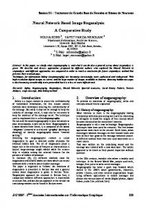
Equation 18 allows us to compute the gradient efficiently and in a scalable manner. All popular GPU programming frameworks provide libraries for scalable convolutions. Figure 1 illustrates the gradient computation for the visualization loss. 4.2.3

Regularized training algorithm

Training requires computing the gradient for the regularized loss function with respect to the parameters of the network. As evident from equation 10, the gradient of the loss function can be computed by first computing the gradients of Lc (M, D), L02 (M ) and VL(M ), and then computing their sum. The gradients of Lc (M, D) and L02 (M ) can be computed using back-propagation and partial derivatives respectively. 5

Figure 1: Computation of gradient for visualization loss. ⊗ denotes convolution.

By equation 9, the gradient of VL(M ) is the sum of gradients of VL(wn ) for n ∈ U (M ). Note ∂ that the gradient ∂w VL(wn ) is zero if w ∈ / wn . In other words, the gradient is zero if w does not belong to the set of weights incoming to node n. Hence we only need to compute the gradients ∂ ∂wn VL(wn ) for all n ∈ U (M ). These can be computed using equation 18. The full algorithm described in figure 2. The algorithm can be extended to using dropout and momentum. Computing each zn in figure 2 takes O(|wn |). Consequently, computing the gradient of the VR regularizer takes O(|w|) time, which is of the same order as computing the gradient of the L2 norm regularizer. Thus, the VR regularizer does not impose additional overhead in the computational complexity per iteration.

5

Relationship with Tikhonov regularization

Tikhonov regularization was originally developed for solutions to ill-posed problems [7]. For example, L2 regularization, a special case of Tikhonov regularization is used to compute solutions to regression problems for which rank deficient matrices are encountered while computing their solutions. The solution to regularized least squares regression is given by, w = argmin kXw − yk2 + λkΓwk2 ,

(20)

w

where Γ is the Tikhonov matrix. The L2 regularizer corresponds to Γ = I. Let w be the concatenation of all the weights in wn for n ∈ U (M ). From equation 16, we can P 0 2 = ( t ct wt )2 , where wt ∈ w, see that VL(wn ) is the sum of squared terms of the form wij 0 ct ∈ {−1, 0, 1} and w0 = wn ⊗ K. For example wij = (wi − wj − wk )2 can be represented in the given form where ci = 1, cj = −1, ck = −1, and all other ct are zero. The Tikhonov matrix Γ can be constructed as follows. Consider the expression of VL(M ) = P ) consisting of the sum of p such squared terms. Let the ith term in this exn∈U (M ) VL(wnP pression be si = ( t cit wt )2 . Then, Γ and consequently VL(M ) in terms of Γ are, respectively, Γ = [cit ]it , and VL(M ) = kΓwk2 .

(21)

The expression of si consists of only a constant number of non-zero cit . The maximum number of non-zero cit is bounded by the maximum number of neighbors a pixel can have, which is 8. Hence, the number of non-zero entries in Γ is O(p), whereas the total number of entries in Γ is p|w|. This establishes the sparsity of Γ. 6

1: procedure T RAIN(D, M, K, µ, λ, α) 2: . D: the training data, M : the model respectively. 3: . K: Kernel for the VR regularizer. 4: . µ: VR regularizer weight, λ: L2 regularizer weight. 5: . α: learning rate. 6: . Returns trained model M 7: 8: . Get the weight variables from the model 9: w := w(M ) 10: Initialize w 11: 12: while does not converge do 13: for minibatch sample Dm do 14: . Step 1: Compute using back-propagation. 15: u ← ∇w Lc (Dm , M ) 16: . Step 2: Gradient for L2 regularizer. 17: v ← ∇w L02 (M ) 18: 19: . Step 3: Gradient for VR regularizer. 20: . Iterate over the nodes in the 1st fully connected layer. 21: for n ∈ U (M ) do ∂ 22: . Compute zn = ∂w VL(wn ) n 23: . using equation 18 24: zn = 2((wn ⊗ K) ⊗ K I ) 25: end for 26: . Concatenate the gradients. 27: z = (. . . , zn , . . . ) 28: 29: . Step 4: Compute total gradient. 30: g ← u + λv + µz 31: . Step 5: Take step. 32: w ← w − αg 33: end for 34: end while 35: return M 36: end procedure

Figure 2: Regularized training algorithm

7

6

Experiments and observations

We experimented on the MNIST [8] and CIFAR-10 [9] datasets and compared the classification accuracy of our algorithm using the VR regularizer with other regularizers.1 6.1

Experimental setting

We used a neural network with two fully connected hidden layers for both the datasets. For the CIFAR-10 dataset, we additionally used a convolution and max pooling layer before the fully connected layers. For simplicity in searching for optimal parameters, we fixed the number of fully connected hidden layers to two, with the number of nodes in each hidden layer equal to 1000. We also fixed the number of feature maps of the convolution layer to 10, and the kernel size to 3 × 3. We used the laplacian kernel for the VR regularizer defined as follows. # " −1 −1 −1 K = −1 8 −1 −1 −1 −1

(22)

We used the mean cross-entropy loss over the mini-batch examples as the classification loss, mean of squares of the weight parameters as the L2 regularizer, and VLm (M ) as the VR regularizer. We trained the neural network using stochastic gradient descent as described in figure 2, and also used Nesterov’s accelerated gradient (momentum) [11]. Note that the first fully connected layer is connected to the input for MNIST, whereas it is connected to the max-pooling layer in the case of CIFAR-10. Thus for the CIFAR-10 network, U (M ) is defined as the set of nodes in the first fully connected layer. The VR regularizer utilizes this modified definition of U (M ) in the case of CIFAR-10. We fixed the number of training epochs to 200 and a mini-batch size of 100. For both MNIST and CIFAR-10, we reduced the learning rate by a factor of 10, respectively after every 100 and 70 epochs. We fixed the momentum parameter to 0.9 and dropout rate to 0.3 for both hidden layers. 6.2

Accuracy

We compared the different neural networks with combinations of L2, VR, and dropout regularizers. For finding the optimal parameters, we performed a randomized hyper-parameter search with manual fine-tuning. The accuracy and optimal hyper-parameters for various regularizer settings are given in table 2. The parameters µ, λ and α respectively denote the VR regularizer weight, the L2 regularizer weight, and the learning rate. From the table it is observed that the VR regularizer is an improvement over the standard L2 regularizer. This is observed both for MNIST and CIFAR-10. 6.3

Convergence

Figures 3 and 4 show the variation of the test set accuracy over the training epochs. Figures 5 and 6 show the variation of the regularization terms over the training epochs. Since loss values for different parameter settings can be of different orders of magnitude, for purposes of visualization, the loss values have been linearly transformed, so as to map to 1 after the first epoch and map to 0 after the last epoch. 6.4

Visualizations of hidden nodes

Figure 7 shows the visualizations of the internal nodes of the MNIST classifier. The first two rows of the sub-figures correspond to nodes in the first hidden layer, and the last two rows correspond to nodes in the second hidden layer. 1

The experiment code is publicly available at https://github.com/biswajitsc/VisRegDL

8

Table 2: Accuracies for various regularizer settings Dataset MNIST

CIFAR-10

Regularizers

µ

λ

α

Accuracy %

L2

-

20

0.1

98.54

L2, VR

1

20

0.1

98.70

Dropout

-

-

0.005

98.50

L2, Dropout

-

1

0.01

98.57

VR, Dropout

1

-

0.01

98.64

L2, VR, Dropout

1

10

0.01

98.58

L2

-

500

0.01

66.62

L2, VR

20

500

0.01

66.85

Dropout

-

-

0.001

64.75

L2, Dropout

-

10

0.001

64.27

VR, Dropout

100

-

0.005

69.54

L2, VR, Dropout

300

10

0.005

71.54

MNIST

0.988

Test accuracy

0.986 0.984 0.982 L2 VR−L2 DR L2−DR VR−DR VR−L2−DR

0.98 0.978 0.976

20

40

60

80

100 120 Epochs

140

160

180

Figure 3: MNIST test set accuracy over iterations. CIFAR−10

0.75

Test accuracy

0.7

0.65

L2 VR−L2 DR L2−DR VR−DR VR−L2−DR

0.6

0.55

0.5

20

40

60

80

100 120 Epochs

140

160

180

Figure 4: CIFAR-10 test set accuracy over iterations.

9

MNIST Total Loss

MNIST VR Loss 2.5 Normalized Loss Value

Normalized Loss Value

1 0.8 0.6 0.4 0.2 0 0 10

2 1.5 1 0.5 0 −0.5

1

10 Epochs

0

2

10

10

1

10 Epochs

2

10

MNIST L2 Loss

Normalized Loss Value

1 L2

0.5

VR−L2 0

DR L2−DR

−0.5

VR−DR −1

VR−L2−DR

−1.5 0

10

1

10 Epochs

2

10

Figure 5: MNIST loss values over iterations. CIFAR−10 VR Loss 1.2

0.8 0.6 0.4 0.2 0 0 10

1 Normalized Loss Value

CIFAR−10 Total Loss

Normalized Loss Value

Normalized Loss Value

1

1 0.8 0.6 0.4 0.2 0

1

10 Epochs

2

0

10

10

1

10 Epochs

CIFAR−10 L2 Loss

0.8

L2 VR−L2

0.6

DR L2−DR

0.4

VR−DR 0.2 0 0 10

VR−L2−DR

1

10 Epochs

2

10

Figure 6: CIFAR-10 loss values over iterations.

10

2

10

(a) L2

(b) VR-L2

(c) L2-DR

(d) VR-L2-DR

Figure 7: Node visualizations of hidden nodes of the MNIST classifier. The first two rows correspond to first hidden layer. The last two rows correspond to the second hidden layer.

The difference between the visualizations of networks trained using the VR regularizer and the ones not trained using it is apparent. The visualizations of architectures using VR regularizer are smoother and less noisy as was expected.

7

Conclusion and future work

We observe that the VR regularizer is an improvement over the popular L2 regularizer in terms of classification accuracy. It is also observed that the networks trained using a VR regularizer have smoother visualizations. Though the VR regularizer imposes the smoothness constraint only on the first hidden layer nodes, our observations from figure 7 show that the smoothness constraint is propagated to the next layer. The VR regularizer may be extended to a new class of training algorithms which use domain knowledge in the form of regularizers.

References [1] S. J. Nowlan and G. E. Hinton, “Simplifying neural networks by soft weight-sharing,” Neural computation, vol. 4, no. 4, pp. 473–493, 1992. [2] D. Erhan, Y. Bengio, A. Courville, P.-A. Manzagol, P. Vincent, and S. Bengio, “Why does unsupervised pre-training help deep learning?,” The Journal of Machine Learning Research, vol. 11, pp. 625–660, 2010. [3] N. Srivastava, G. Hinton, A. Krizhevsky, I. Sutskever, and R. Salakhutdinov, “Dropout: A simple way to prevent neural networks from overfitting,” The Journal of Machine Learning Research, vol. 15, no. 1, pp. 1929–1958, 2014. [4] J. Ba and B. Frey, “Adaptive dropout for training deep neural networks,” in Advances in Neural Information Processing Systems, pp. 3084–3092, 2013. 11

[5] Y. LeCun, Y. Bengio, and G. Hinton, “Deep learning,” Nature, vol. 521, no. 7553, pp. 436–444, 2015. R in Machine Learn[6] Y. Bengio, “Learning deep architectures for ai,” Foundations and trends ing, vol. 2, no. 1, pp. 1–127, 2009.

[7] A. Tikhonov and V. Arsenin, Solutions of ill-posed problems. VH Winston and Sons, 1977. [8] Y. LeCun and C. Cortes, “The MNIST database of handwritten digits,” 1998. [9] A. Krizhevsky, “Learning multiple layers of features from tiny images,” Technical Report, Univ. Toronto, 2009. [10] D. Erhan, Y. Bengio, A. Courville, and P. Vincent, “Visualizing higher-layer features of a deep network,” Technical Report, Univ. Montreal, 2009. [11] Y. Nesterov, “A method of solving a convex programming problem with convergence rate {O}(1/kˆ2),” Soviet Mathematics Doklady, vol. 27, no. 2, pp. 372–376, 1983.

12