Neural Network-based Chaotic Pattern Recognition - International ...

Neural Network-based Chaotic Pattern Recognition- Part 2: Stability and Algorithmic Issues D. Calitoiu1 , B. John Oommen2 , and D. Nussbaum1 1

2

School of Computer Science, Carleton University, K1S 5B6, Canada, {dcalitoi, nussbaum}@scs.carleton.ca Fellow of the IEEE, School of Computer Science, Carleton University, [email protected]

Summary. Traditional Pattern Recognition (PR) systems work with the model that the object to be recognized is characterized by a set of features, which are treated as the inputs. In this paper, we propose a new model for Pattern Recognition (PR), namely, one that involves Chaotic Neural Networks (CNNs). To achieve this, we enhance the basic model proposed by Adachi [1], referred to as Adachi’s Chaotic Neural Network (ACNN). Although the ACNN has been shown to be chaotic, we prove that it also has the property that the degree of “chaos” can be controlled; decreasing the multiplicity of the eigenvalues of the underlying control system, we can effectively decrease the degree of chaos, and conversely increase the periodicity. We then show that such a Modified ACNN (M-ACNN) has the desirable property that it recognizes various input patterns. The way that this PR is achieved is by the system essentially sympathetically “resonating” with a finite periodicity whenever these samples are presented. In this paper, which follows its companion paper [2], we analyze the M-ACNN for its stability and algorithmic issues. This paper also includes more comprehensive experimental results.

1 Introduction Traditional Pattern Recognition (PR) systems work with the model that the object to be recognized is characterized by a set of features, which are treated as the inputs. We propose a now model of PR, namely Chaotic PR. This paper follows a companion paper [2] in which we earlier presented some analytic stability properties of the Chaotic PR systems, using Lyapunov Exponents. In [2], we had also presented some elementary PR results involving a few patterns, essentially the patterns discussed by Adachi [1]. In this paper, we analyze the stability of the model using the Routh-Hurwitz Criterion, we present algorithmic issues, and also the experimental results for a more “reallife” data set involving numerals.

4

D.Calitoiu et al.

Pattern Recognition (PR) is the study of how a system can observe the environment, learn to distinguish patterns of interest from their background, and make decisions about their classification or categorization. In general, a pattern can be any entity described with features, where the dimensionality of the feature space can range from being few to thousands. The four best approaches for PR are: template matching, statistical classification, syntactic or structural recognition, and Artificial Neural Networks (ANNs) [4],[5],[6],[7],[8]. The latter approach attempts to use some organizational principles such as learning, generalization, adaptivity, fault tolerance and distributed representation, and computation in order to achieve the recognition. The main characteristics of ANNs are that they have the ability to learn complex nonlinear input-output relationships, use sequential training procedures and adapt themselves to data. Some popular models of ANNs have been shown to be capable of associative memory and learning [9],[10],[11]. The learning process involves updating the network architecture and modifying the weights between the neurons so that the network can efficiently perform a specific classification/clustering task. An associative memory permits its user to specify part of a pattern or key, and to thus retrieve the values associated with that pattern. One of the limitations of most ANN models of associative memory is the dependency on an external input. Once an output pattern has been identified, the ANN remains in that state until the arrival of an external input. This is in contrast to real biological neural networks which exhibit sequential memory characteristics. To be more specific, once a pattern is recalled from a memory location, the brain is not “stuck” to it, it is also capable of recalling other associated memory patterns without being prompted by any additional external stimulus. This ability to “jump” from one memory state to another in the absence of a stimulus is one of the hallmarks of the brain, and this is one phenomenon that we want to emulate. The evidence that indicates the possible relevance of chaos to brain functions was first obtained by Freeman [13],[14] through his clinical work on the large-scale collective behavior of neurons in the perception of olfactory stimuli. Freeman developed a model for an olfactory system having cells in a network connected by both excitatory and inhibitory synapses. He described how a chaotic system state in the neighborhood of a desired attractor can fall on a stable direction when a perturbation is applied to a system parameter. From this model, he conjectured that the quiescent state of the brain is chaos, while during perception, when attention is focused on any sensory stimulus, the brain activity becomes more periodic. The periodic orbits observed can be interpreted as specific memories. If the patterns stored in memory are identified with an infinite number of unstable periodic attractors which are embedded in an attractor, then the transition from the quiescent state onto an “attention” state can be interpreted as the controlling of chaos. The controlling of chaos gives rise to periodic behavior, culminating in the identification of the sensory stimulus that has been received. Thus, mimicing this identification on

Stability and Algorithmic Issues: Chaotic PR.

5

a neural network can lead to a new model of pattern recognition, which is the goal of this research endeavor3 . During its evolution, a CNN with fixed weights can be in one of the infinite states within the precomputed state space volume. In the case when one inserts one of the memorized patterns as an input in the network, we want the network to resonate with that pattern, generating that pattern with a certain periodicity. Between two consecutive appearances of the memorized pattern, the network can also be in an infinite number of states, but in none of the memorized ones. The resonance with the memorized pattern given as input, and the transition through several states from the infinite set of possible states (even when the memorized pattern is inserted as input) represent the difference between this kind of pattern recognition and the classical type which corresponds to the strategies associated with statistical, syntactical or structural PR. This is explained in greater detail in [2] and [3], where we also show that in order to achieve recognition, one must decrease the level of chaos until periodic behavior is obtained. 1.1 Contributions of this paper The primary contribution of this paper is the introduction of a PR system which is founded on the theory of chaotic networks. However, rather than relying only on the chaos of the system, we have shown that chaos and periodicity are, informally, “negotiable” quantities. A more chaotic network leads to a weak PR system and vice versa. In particular, by modifying Adachi’s model, we anlyze the dynamics of a new model of chaotic neural networks, the M-ACNN with a PR behavior superior to that of the ACNN. We especially focus on the stability of the network and the retrieval characteristics in the transient dynamics of the network. The latter is analyzed by considering the frequencies of retrieval and the transitions among the stored patterns. This allows us to clarify the ability of the memory searching process. Adachi [1] explained that when the duration of the transient phase is long, the attracting state after such a long transient phase may not be useful for information processing. We have shown that by increasing the multiplicity of the eigenvalues of the ACNN, the PR property of the network can be enhanced, leading to the system resonating “sympathetically” whenever a reasonable version of a stored pattern is presented. Thus, the ACNN has a higher level of chaos then the M-ACNN but the recognition is superior in the latter, because the M-ACNN is more stable. Earlier, in [2] we presented some analytic stability properties of the Chaotic PR systems, using Lyapunov Exponents. In this paper, we analyze the stability of the model using the Routh-Hurwitz criterion, 3 Unfortunately, if the external excitation forces the brain out of chaos completely, it can lead to an epileptic seizure, and a future goal of this research is to see how these episodes can be anticipated, remedied and/or prevented.

6

D.Calitoiu et al.

we present algorithmic issues and also the experimental results for a more “real-life” data set involving numerals.

2 Adachi model of chaotic neural networks: ACNN The ACNN is composed of N neurons (Adachi set N = 100), topologically arranged as a completely connected graph i.e, each neuron communicates with every other neuron, including itself. The ACNN is modelled as a dynamical associative memory, by means of the following equations relating the two internal states ηi (t) and ξi (y), i = 1..N , and the output xi (t) as: xi (t + 1) = f (ηi (t + 1) + ξi (t + 1)),

ηi (t + 1) = kf ηi (t) +

N X

(1)

wij xj (t),

(2)

ξi (t + 1) = kr ξi (t) − αxi (t) + ai .

(3)

j=1

In the above, xi (t) is the output of the neuron i which has an analog value in [0,1] at the discrete time “t”. The internal states of the neuron i are ηi (t) and ξi (t), f is the logistic function with the steepness parameter ε satisfying f (y) = 1/(1 + exp(−y/ε)). Additionally, 1. kf and kr are the decay parameters for the feedback inputs and the refractoriness, respectively, 2. wij are the synaptic weights to the ith constituent neuron from the j th constituent neuron, and 3. ai denotes the temporally constant external inputs to the ith neuron. While the network dynamics are described by Equation (2) and Equation (3), the outputs of the neurons are obtained by Equation (1). The feedback interconnections are determined according to the following symmetric autoassociative matrix of the p stored patterns as in: p

1X s wij = (2x − 1)(2xsj − 1), p s=1 i

(4)

where xsi is the ith component of the sth stored pattern.

3 A new model of chaotic neural networks: M-ACCN We propose a new model of chaotic neural networks which modify the ACNN as below. In each case we give a brief rationale for the modification.


7

1. The M-ACNN has two global states used for all neurons, which are η(t) and ξ(t) obeying: xi (t + 1) = f (ηi (t + 1) + ξi (t + 1)),

ηi (t + 1) = kf η(t) +

N X

(5)

wij xj (t),

(6)

ξi (t + 1) = kr ξ(t) − αxi (t) + ai .

(7)

j=1

After each step t + 1, the global states are updated with the values of ηN (t + 1) and ξN (t + 1): η(t + 1) = ηN (t + 1)

(8)

ξ(t + 1) = ξN (t + 1).

(9)

Rationale: Note that at every time instant, when we compute a new internal state, we only use the contents of the memory from the internal state for neuron N . This is in contrast to the ACNN in which the updating at time t+1 uses the internal state values of all the neurons at time t. Observe that this, as can be anticipated, could cause the CNN to be “less chaotic”, as we shall see presently. 2. The weight assignment rule for the M-ACCN is the classical variant: p

1X s s (x )(x ) p s=1 i j

(10)

ai = 1, if xsi = 1

(11)

wij =

Pp This again, is in contrast to the ACNN which uses wij = p1 s=1 (2xsi − 1)(2xsj − 1). Rationale: We believe that the duration of the transitory process will be short if the level of chaos is low. Shuai [16] explained that a simple way to construct hyperchaos with all Lyapunov positive exponents is to couple N chaotic neurons, and to set the couplings between the neurons to be small when compared with their self-feedbacks, i.e wii À wij (i 6= j). In the ACNN, if for any i,j, (where 1 ≤ i, j ≤ N ) the value xsi = xsj = 0 for all s, then wi,i will be unity. However, for the M-ACNN, the value of wi,i will be zero in the identical setting. Clearly, the M-ACCN has a smaller self-feedback effect than the ACNN. 3. The external inputs are applied in the M-ACNN, only to the neurons representing the stored pattern, by increasing their biases, ai , from 0 to unity whenever xsi = 1. The biases to the other neurons remain to be 0. Thus

8

D.Calitoiu et al.

ai = 0, otherwise.

(12)

In other words, in our case ai = xsi , as opposed to the ACNN in which ai = 2 + 6xsi . Rationale: The M-ACCN is more sensitive to the external input than the ACNN. The range of input values is between 0 and unity in the M-ACCN, in contrast with the range of input values being between 2 and 8 in the A-CNN. Thus, the M-ACNN will be more “receptive” to external inputs, leading to, hopefully, a superior PR system.

4 The M-ACNN orbital instability The stability of the Chaotic PR system which we proposed, has been analyzed by two methodologies listed below. The first, which uses the Lyapunov Exponents and their properties, is given in the companion paper [2] and in [3]. The second, which utilizes the Routh-Hurtwitz criterion, is explained in great details below and in [3]. 4.1 Analysis using Lyapunov Exponents For a dynamical system, sensitivity to initial conditions is quantified by the Lyapunov exponents. For example, consider two trajectories with nearby initial conditions on an attracting manifold. When the attractor is chaotic, the trajectories, on average, diverge at an exponential rate characterized by the largest Lyapunov exponent. This concept is also generalized for the spectrum of Lyapunov exponents. The presence of positive exponents is sufficient for diagnosing chaos and represents local instability in particular directions [?]. In this regard, the M-ACNN has the following property. Theorem 1. The M-ACNN described by Equations (6) and (7) is locally more stable than the ACNN, as demonstrated by their Lyapunov spectrums. In the interest of brevity, the proof is found in [2], the companion paper. 4.2 Analysis using the Routh-Hurwitz Criterion We consider a physical system described by a set of simultaneous equations dAi = fi (A1 , A2 , · · · , Ar ) with i = 1..r, dt

(13)

where fi are general nonlinear functions of the dependent variables A1 , · · · , Ar . A state of equilibrium may be represented by a singular point or a limit cycle of Equation (13). The Routh-Hurwitz (RH) criterion is applicable only to an


9

equilibrium point where all the derivates of A1 , · · · , Ar with respect to t are simultaneously zero. Under this condition we obtain: fi (A1 , A2 , · · · , Ar ) = 0 for all i = 1..r;

(14)

If the system is linear, we obtain a single set of values for variables {Ai } satisfying Equation (14). Hence the state of equilibrium is uniquely fixed. But since our system is nonlinear, Equation (14) may be satisfied for more than a single set of values for the variables {Ai } inasmuch as nonlinear systems may have a number of equilibrium states. In order to investigate the stability of a system near a chosen equilibrium point, we apply a sufficiently small disturbance to the system by changing the Ai ’s from their equilibrium values. Then, if t increases infinitely and all the Ai ’s return to their original equilibrium values, the system is asymptotically stable at this equilibrium point. On the other hand, if some/all of the Ai ’s depart from their original stable values with increasing t, the system is unstable. We now state some chaos-related properties of the M-ACNN using the RH criterion. The detailed proof can be found in [3]. Theorem 2. The M-ACNN described by Equations (6) and (7) is locally unstable. Sketch of Proof: Let us denote a set of equilibrium values for the MACNN for the Ai ’s by A10 , A20 · · · Ar0 . Consider now small variations ε defined by: A1 = A10 + ε1 ; A2 = A20 + ε2 ; · · · Ar = Ar0 + εr ;

(15)

Substituting Equation (15) in Equation (13) and discarding terms of smaller significance than of the first order in ε we get: dε1 = c11 ε1 + c12 ε2 + ... + c1r ²r . dt dε2 = c21 ε1 + c22 ε2 + ... + c2r ²r . dt dεr ··· = cr1 ε1 + cr2 ε2 + ... + crr ²r . dt

(16) (17) (18)

∂(fi ) where cij stands for ∂(A at the equilibrium state A1 = A10 , · · · Ar = Ar0 . j) We know [12] that, if the real parts of the roots of the characteristics equation of the system Equation (16)-(18) are negative, the corresponding equilibrium state is stable, and conversely, if at least one root has a positive real part, the equilibrium is unstable. Consider now the characteristic equation given by Equation(16)-(18). When expanded, this rth -order determinant leads to an equation of the form:

10

D.Calitoiu et al.

c0 λr + c1 λr−1 + ... + cr−1 λ + cr = 0.

(19)

The determination of signs of the real parts of the roots of λ may be carried out by making use of the RH criterion. To apply this criterion, we first construct a set of r determinants set up from the coefficients of the rth -degree characteristic equation as shown in Equation (19). The RH criterion states that the real part of the roots λ are negative provided that all the coefficients c0 , c1 , ... cr are positive, and that all the determinants ∆1 , ∆2 , ... ∆r are positive. Since the bottom row of the determinant ∆r is composed entirely of zeros, except for the last element cr , it follows that ∆r = cr ∆r−1 . Thus, for stability it is required that both cr > 0 and ∆r−1 > 0, and ∆r need not actually be evaluated. In the case of the M-ACNN, the Jacobian matrix for the system generates a characteristic equation: λ2N − (kf + kr )λ2N −1 + kf kr λ2N −2 = 0

(20)

∆1 = det(c1 ) = −(kf + kr )

(21)

and Clearly the sign of the ∆1 depends on the magnitude of the coefficients kf and kr . This theorem follows since kf > 0 and kr > 0. u t Remarks: 1. The computation of ∆1 is non-trivial for the ACNN. The first two terms of the the characteristic equation are : λ2N and (kf + kr )N (−1)N −1 λ2N −1 respectively. In this case, ∆1 , which is equal to (kf + kr )N (−1)N −1 , depends on the magnitude of the coefficients kf and kr , and the value of N . It appears as if Adachi et al.[1] proved the instability of the ACNN empirically and not analytically. 2. Adachi et al.[1] have found that the best parameters for their data set are kf = 0.2 and kr = 0.9. Our experiments confirm this.

5 Designing Chaotic PR Systems To attempt to design PR systems based on the brain model suggested by Freeman [14],[13] is no easy task. Typically, PR systems work with the following model: given a set of training patterns, the PR system learns the characteristics of the class of the patterns, and this information is retained either parametrically or non-parametrically. When a testing sample is presented to the system, a decision of the identity of the class of the sample is made using the corresponding “discriminant” function, and this class is “proclaimed” by the system as the identity of the pattern. The same philosophy is also true for syntactic/structural PR systems.


11

As opposed to this, we do not expect chaotic PR systems to report the identity of the testing pattern with such a “proclamation”. Rather, what we are attempting to achieve is to have the chaotic PR system continuously demonstrate chaos as long as there is no pattern to be recognized, or whenever a pattern that is not to be recognized is presented. But, when a pattern which is to be recognized is presented to the system, we would like the proclamation of the identity to be made by requiring that the system simultaneously resonates sympathetically. To be more specific, let us suppose that we want the chaotic PR system to recognize patterns Pi and Pj . To accomplish this, we shall train the system using these patterns. It is interesting to observe what this training accomplishes. By a mere straightforward computation (as opposed to an iterative computation) this training phase assigns the weights between the neurons of the CNN. These weights effectively memorize the training patterns so that the network, in turn, effectively behaves as an “Associative Memory” system. Subsequently, on testing, if any pattern other than Pi or Pj is presented, the CNN must continue to be chaotic, since it is not trained to recognize such a pattern. However, if Pi or Pj , (or a pattern resembling either of them) is presented, the CNN must switch from being chaotic to being periodic. Note that as opposed to traditional PR systems, the output is not a single value. It is a sequence of values, which is chaotic (i.e., displays no periodicity) unless one of the trained patterns is presented. In the latter case, the system switches to being periodic, and by examining the periodicity in the system, the user must be able to infer that one of the stored patterns has been encountered, and thus infer the identity of the pattern. Adachi et al. [1] had suggested, rather informally, that such a chaotic PR system could be developed. However, the mechanics of the system were not fully explained. The problem with Adachi’s ACCN is that it is “extremely” chaotic, and there seems to be no easy way by which the level of chaos can be controlled. This is exactly what we can also deduce from the above two theorems. In order to develop a PR system from Adachi’s model, we must be able to decrease the level of chaos in a controlled manner while we simultaneously increase the stability. This is the rationale for the M-ACNN. By decreasing the number of kf and kr terms along the principal diagonal of the dynamical matrix, we can effectively increase the multiplicity of the eigenvalue “0”. This multiplicity (of the eigenvalue “0”) can be increased from the value 0 to the value 2N −2 depending on the number of terms we choose to include along the principal diagonal. In the limit, we could design the CNN so as to have only one entry of kf and kr along the diagonal, thus forcing all the other eigenvalues to be exactly zero. Observe that by virtue of the theorems proven, the corresponding stability also increases. This will thus, in turn, lead to a chaotic system which can switch to become periodic and stable if it is presented with a testing sample resembling one for which it has been appropriately trained. This is exactly what we have achieved.

12

D.Calitoiu et al.

The formal procedure for the PR system is as explained above, and is found algorithmically as follows below: Algorithm PR using M-ACNN Begin Module Training Input: The set of training patterns S = {X 1 · · · X p } with X i = [xi1 · · · xiN ]. Output: The weights of the M-ACNN. Method: /* Compute the weights using the set of training patterns */ FOR i = 1 to N FOR j = 1 to N wij = 0; FOR s = 1 to p wij = wij + xsi xsj ENDFOR ENDFOR ENDFOR End Module Training Begin Module Testing Input: A pattern Y Output: A periodic sequence of one (or more) of the memorized patterns X f if Y = [y1 · · · yN ]T is close X f . The sequence must not contain any memorized pattern if Y is “far away” from any {X s } with s = 1..p. The output of the M-ACNN is given by U = [u1 · · · uN ] obeying (2)-(4). Criterion: Y is considered “close” to any X s if the noise level is less than a predefined value, Threshold. Method: /*Read input pattern Y = [y1 · · · yN ] */ FOR i=1 to N ai = yi ENDFOR /*Compute the output using the dynamical equations (2)-(4) */ η(0) = 0; ξ(0) = 0; cf = 0; /* initialize the periodicity counter for the training set */ FOR f = 1 to p count(f, cf ) = 0 ENDFOR FOR t = 0 to Nmax FOR i = 1 to N P100 ηi (t + 1) = kf η(t) + j=1 wij uj (t); ξi (t + 1) = kr ξ(t) − αui (t) + ai ; ui (t + 1) = f (ηi (t + 1) + ξi (t + 1)); ENDFOR


13

η(t + 1) = ηN (t + 1) ξ(t + 1) = ξN (t + 1) /* Compute the distance between the output U and each pattern X s */ FOR s = 1 to p ds (t) = 0; ENDFOR FOR s = 1 to p FOR i=1 to N ds (t) = ds (t) + |(ui (t) − xi s )| ENDFOR /* we accept a level of noise for Y , equal to (T hreshold/N )% */ IF ds (t) ≤ T hreshold f =s /*index of recognized pattern X f , close to Y */ count(f, cf ) = t; cf = cf + 1; ENDIF ENDFOR ENDFOR /* Test the periodicity for only 2 cycles */ periodicity[f ] = count(f, 2) − count(f, 1) Report index f and periodicity[f ]. End Module Testing End Algorithm PR using M-ACNN

6 Experimental results In the training phase, as mentioned earlier, we present the system with a set of patterns, and thus by a sequence of simple assignments (as opposed to a sequence of iterative computations), it “learns” the weights of the CNN. The testing involves detecting a periodicity in the system, and then inferring what the periodic pattern is. We shall now demonstrate how the latter task is achieved. In a simulation setting, we are not dealing with a real-life chaotic system. Indeed, in this case, the output of the CNN is continuously monitored, and the only way by which a periodic behavior can be observed, is to keep track of all the outputs as they come. Notice that this is an infeasible task, as the number of distinct outputs could be countably infinite. This is a task which the brain, (or, in general, a chaotic system), seems to be able to do, quite easily, and in multiple ways. However, since we have to work with serial machines, to demonstrate the periodicity, we have no choice but to compare the output patterns with the various trained patterns. Whenever the distance between the output pattern and any trained pattern is less than a threshold, we mark that time instant with a distinct marker characterized by the class of that particular pattern. The question of determining the periodicity of a pattern is now merely one of determining the periodicity of these markers.

14

D.Calitoiu et al.

To present our results in the right perspective, we have tested the schemes for two sets of data. The first was precisely the set which Adachi and his co-authors used [1]. These results are presented in [2], the companion paper. The second set is more realistic, and is one which involves the recognition of numerals. We report here only the results obtained from the second data set. 6.1 PR with a Numeral Data Set

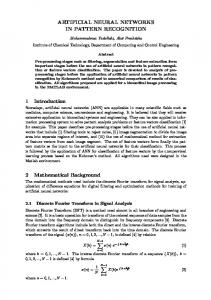
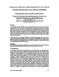
Fig. 1. The second set of patterns used in the PR experiments. These were the 10 × 10 bitmaps of the numerals 0 · · · 9. The initial state used was randomly chosen.

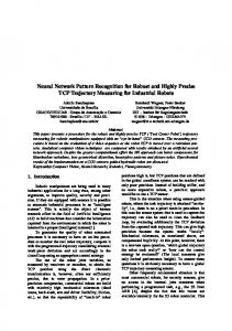
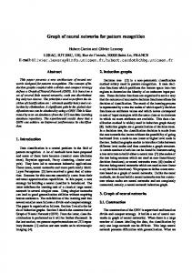
We conducted numerous experiments on a numeral dataset described below. The training set had 10 patterns, given in Fig. 1, and consisted of 10 × 10 bit-maps of the numerals 0 · · · 9. The parameters used were: N = 100 neurons, ε = 0.00015, α = 10, kf = 0.2 and kr = 0.9 for Equations (5)-(7). The numeral data set was tested for cases when noise was included in the bitmaps. After the training, the system was presented with 10×10 binary-valued arrays which contained noisy versions of one of the numerals.The noise in each case was measured by the percentage of pixels which were modified from 0 to 1 and vice versa. Thus, if the noise was 15%, 15 (out of the 100) randomly chosen pixel values (say, xpi ) of X p were modified and were rendered different from those in the original pattern, X p . Numerous tests were done, but in the interest of simplicity, we merely mention the case when the noise was 15%, as presented in Fig. 2. After an initial (rather insignificant) non-periodic transient phase, with a mean length of 9.1 time units, the system resonated sympathetically. In this case, the PR accuracy was 100%. The actual values of the duration of the transitory phases and the respective periods are given in Table 1. In our opinion, the results


15

are remarkable, especially when we observe the extremely poor quality of the testing samples. Table 1. The transitory phase and the periodicity for M-ACNN, when the testing is done with patterns from the training set containing 15% noise. Note that some patterns have limit cycles with multiple periods. Pattern No of steps in transitory process Periodicity 1 2 3 4 5 6 7 8 9 10

24 8 8 8 8 8 8 8 8 7

25 7,7,8 7,7,8 7,7,8 7,7,8 7,7,8 7,7,8 7,7,8 2,5,7,8 22

Fig. 2. The second set of patterns with 15% noise, used in recognition.

7 Conclusion In this paper, we have proposed a new model for PR, namely one that involves Chaotic Neural Networks (CNNs). To achieve this, we enhanced the basic model proposed by Adachi [1], referred to as Adachi’s Chaotic Neural Network (ACNN). Although the original ACNN has been shown to be chaotic,

16

D.Calitoiu et al.

we have shown that it also has the fascinating property that it can be modified so that the degree of “chaos” can be controlled by decreasing the multiplicity of the eigenvalues of the underlying control system. By modifying the original ACNN, we have designed the Modified ACNN (M-ACNN) which “resonates” with a finite periodicity whenever the training samples (or their reasonable resemblances) are presented. Apart from analyzing the M-ACNN for its periodicity, stability and the length of the transient phase of the retrieval process, we have also demonstrated its PR capability by testing it on Adachi’s dataset, and also for a real-life PR problem involving numerals. The accuracy in each case was a perfect 100%.

References 1. Adachi M, Aihara K (1997) Associative Dynamics in a Chaotic Neural Network, Neural Networks 10:83–98 2. Calitoiu D, Oommen BJ, Nussbaum D (2005) Neural Network-based Chaotic Pattern Recognition - Part 1: Lyapunov Stability and Periodicity Issues, Submitted for PRIP’2005 (Eight International Conference on Pattern Recognition and Information Processing), Minsk, Belarus 3. Calitoiu D, Oommen BJ, Nussbaum D, Periodicity and Stability Issues of a Novel Chaotic Pattern Recognition Neural Network, Submitted for Publication, Unabridged version of the Paper 4. Theodoridis S, Koutroumbas K (1999) Pattern recognition. Academic Press 5. Bishop C M, Bishop C(2000) Neural Networks for Pattern Recognition. Oxford University Press 6. Ripley B (1996) Pattern Recognition and Neural Networks. Cambridge University Press 7. Fukunaga K (1990) Introduction to Statistical Pattern Recognition. Academic Press 8. Friedman M, Kandel A (1999) Introduction to Pattern Recognition, statistical, structural, neural and fuzzy logic approaches. World Scientific 9. Schurmann J (1996) Pattern classification, a unified view of statistical and neural approaches. John Wiley and Sons, New York 10. Kohonen T (1997) Self-Organizing Maps. Springer, Berlin 11. Fausett L (1994) Fundamentals of Neural Networks. Prentice Hall 12. Minorsky N (1962) Nonlinear Oscillations. D.Van Nostrand Company 13. Skarda CA, Freeman WJ (1987) How brains make chaos to make sense of the world, Behavioral and Brain Science 10:161–165 14. Freeman WJ (1992) Tutorial in neurobiology: From single neuron to brain chaos, International Journal of Bifurcation and Chaos 2:451–482 15. Shuai JW, Chen ZX, Liu RT, Wu BX (1997) Maximum hyperchaos in chaotic nonmonotonic neuronal networks, Physical Review E 56:890–893 16. Rosenstein MT, Collins JJ, De Luca CJ (1993) A practical method for calculating largest Lyapunov exponents from small data sets ,Physica D 65:117–134 17. Geist K, Parlitz U, Lauterborn W (1990) Comparison of Different Methods for Computing Lyapunov Exponents, Progress of Theoretical Physics 83:875–893