Hindawi Publishing Corporation Advances in Artificial Neural Systems Volume 2013, Article ID 486363, 8 pages http://dx.doi.org/10.1155/2013/486363
Research Article Visualizing Clusters in Artificial Neural Networks Using Morse Theory Paul T. Pearson Department of Mathematics, Hope College, P.O. Box 9000, Holland, MI 49422-9000, USA Correspondence should be addressed to Paul T. Pearson;
[email protected] Received 27 March 2013; Revised 31 May 2013; Accepted 5 June 2013 Academic Editor: Songcan Chen Copyright © 2013 Paul T. Pearson. This is an open access article distributed under the Creative Commons Attribution License, which permits unrestricted use, distribution, and reproduction in any medium, provided the original work is properly cited. This paper develops a process whereby a high-dimensional clustering problem is solved using a neural network and a lowdimensional cluster diagram of the results is produced using the Mapper method from topological data analysis. The lowdimensional cluster diagram makes the neural network’s solution to the high-dimensional clustering problem easy to visualize, interpret, and understand. As a case study, a clustering problem from a diabetes study is solved using a neural network. The clusters in this neural network are visualized using the Mapper method during several stages of the iterative process used to construct the neural network. The neural network and Mapper clustering diagram results for the diabetes study are validated by comparison to principal component analysis.
1. Introduction Topological data analysis (TDA) is an emerging field of mathematics that focuses on constructing topological models for data and calculating algebraic invariants of such models [1–3]. The fundamental idea is to use methods from topology to determine shapes or patterns in high-dimensional data sets [4]. One method from TDA called Mapper constructs a lowdimensional topological model for a data set 𝑋 ⊂ R𝑚 from the clusters in the level sets of a function ℎ : 𝑋 → R𝑛 on the data set [5]. This topological model for 𝑋 is a cluster diagram that shows the clusters in the level sets of ℎ (i.e., clusters in the layers of a stratification of 𝑋) and how clusters in adjacent, overlapping level sets are connected (i.e., how the neighboring layers are glued together). The topological model built in this way is analogous to how Morse theory is used to construct a cell decomposition of a manifold using sublevel sets of a Morse function on the manifold [5–7]. The resolution of the cluster diagram produced by Mapper can be adjusted by changing the level sets by varying the number, size, and shape of the regions used to cover the image of the function ℎ. Further, the Mapper method allows for different clustering algorithms to be used. The most important step for obtaining a useful topological model from Mapper is finding a function
ℎ : 𝑋 → R𝑛 that solves a particular clustering problem of interest for a data set 𝑋. This study examines the case when the function ℎ is a neural network. A feedforward, multilayer perceptron artificial neural network (hereafter called a neural network) is a function 𝑓 : R𝑚 → R𝑛 constructed by an iterative process in order to approximate a training function 𝑔 : 𝑃 → 𝑇 between two finite sets of points 𝑃 and 𝑇 called the inputs and target outputs, where 𝑃 ⊆ 𝑋 ⊂ R𝑚 and 𝑇 ⊂ R𝑛 . In a context where a target output value represents the classification of an input point, the neural network 𝑓 is a solution to a classification or clustering problem because 𝑓 has been trained to learn the rule of association of inputs with target outputs given by 𝑔. In this manner, many clustering problems for high dimensional data sets 𝑋 ⊂ R𝑚 have been solved by finding collections of points in the domain of 𝑓 that have similar output values, which is to say that the level sets of a neural network are solutions to a clustering problem [8–12]. Although neural networks are adept at solving clustering problems, it is hard to visualize these clusters when the neural network’s domain has dimension 𝑚 > 3. To address this limitation, Mapper will be used to construct a low-dimensional, visualizable topological model that shows the clusters in the level sets of 𝑓 as well as how clusters in neighboring level sets are connected. More
2 generally, using Mapper to make a cluster diagram of the level sets of a neural network will provide a low-dimensional picture of the solution to a clustering problem that makes interpreting the neural network results much easier. The research presented in this paper uses the MillerReaven diabetes study data [13, 14] as a case study for the method of using a neural network to solve a clustering problem and Mapper to visualize and interpret the results. A neural network is constructed that classifies patients of a diabetes study as overt diabetic, chemical diabetic, or not diabetic based on the results of five medical tests. The neural network is trained using the five medical tests as inputs and the diagnosis of diabetes type as the target output. At several intermediate stages of the weight update process during the construction of this neural network, the Mapper method is used to create a topological model of the level sets of the neural network at that stage of its formation. The results are compared to principal component analysis (PCA) as a means to validate the method. The general method presented in this paper for solving and visualizing clustering problems combines the efficacy of neural networks, which are nonlinear functions that have a proven track record for solving a wide variety of clustering problems whenever a training function is available [15], with the clarity and simplicity of the cluster diagrams produced by the Mapper method to make the neural network’s solution to the clustering problem readily comprehensible. The Mapper method has been used previously in the context of unsupervised learning by using functions such as density and eccentricity estimates to study diabetes data, breast cancer data, and RNA hairpin folding [4, 5, 16, 17]. Since neural networks employ supervised learning, using neural networks together with Mapper may provide more accurate and precise results than what could be attained by unsupervised learning on the same data. Other techniques for visualization of high-dimensional data sets such as projection pursuit, Isomap, locally linear embedding, and multidimensional scaling are discussed in relation to Mapper in [5]. Methods for visualizing the clusters in a neural network have been constructed by a variety of other dimension reduction techniques. Such techniques include linear and nonlinear projection methods [18], principal component analysis [19], Sammon’s mapping [20], multidimensional scaling and nonlinear mapping networks [21], and fuzzy clustering [22]. These dimension reduction techniques produce useful twoand three-dimensional models of the data set and have varying degrees of success in solving specific real-world problems. Some of these constructions can be quite sensitive to the distance metric chosen, outliers in the data, or other factors. This paper is organized as follows. In Section 2, background information on neural networks is given, followed by a description of the Mapper method from topological data analysis. Section 3 describes the Miller-Reaven diabetes study, principal component analysis, and the configuration of the neural network and Mapper algorithm used to analyze the diabetes data. Section 4 demonstrates the results of applying PCA and a neural network to the diabetes data and compares the PCA results to the cluster diagram for the neural network
Advances in Artificial Neural Systems produced using the Mapper method. Section 5 summarizes the main results of the case study, the general method of using neural networks to solve clustering problems, and the Mapper method to visualize the resulting clustering diagrams.
2. Background This section provides a brief overview of neural networks and the Mapper method from topological data analysis. 2.1. Brief Description of Neural Networks. A neural network is function 𝑓 : R𝑚 → R𝑛 constructed via an iterative process in order to approximate a training function 𝑔 : 𝑃 → 𝑇 between two finite sets of points 𝑃 ⊆ 𝑋 ⊂ R𝑚 and 𝑇 ⊂ R𝑛 called the inputs 𝑃 (which is a subset of a data set 𝑋) and target outputs 𝑇. Neural networks are universal approximators in the sense that for every training function 𝑔, there exists a globally defined neural network 𝑓 that approximates 𝑔 to any desired degree of accuracy [23, 24]. Even though it is possible to find a neural network 𝑓 that approximates 𝑔 to any predetermined degree of accuracy, in practice such a neural network 𝑓 could have a very large network architecture and be impractical. Thus, it is often desirable to find a moderately sized network architecture for 𝑓 that approximates 𝑔 to an acceptable degree of accuracy. This study will examine a neural network with one hidden layer of ℎ1 nodes. Such a neural network 𝑓 : R𝑚 → R𝑛 has the form 𝑓 (𝑥) = 𝑓2 (𝑊2 (𝑓1 (𝑊1 𝑥 + 𝑏1 )) + 𝑏2 ) ,
(1)
where 𝑥 ∈ R𝑚 , 𝑊1 is a ℎ1 × 𝑚 weight matrix, 𝑊2 is a 𝑛 × ℎ1 weight matrix, 𝑏1 is a ℎ1 × 1 bias vector, 𝑏2 is a 𝑛 × 1 bias vector, and 𝑓𝑖 : R → R denotes an activation function. For classification problems with multiple classes of data, it is common to choose 𝑓1 (𝑥) = tanh(𝑥) = (𝑒𝑥 − 𝑒−𝑥 )/(𝑒𝑥 + 𝑒−𝑥 ) and 𝑓2 (𝑥) = 𝑥 as activation functions. An activation function is evaluated on a vector by applying the function to each entry of the vector. The iterative process for constructing a neural network 𝑓 : R𝑚 → R𝑛 from a training function 𝑔 : 𝑃 → 𝑇 begins by initializing the weights 𝑊𝑖 and biases 𝑏𝑖 with random values. Points 𝑝 ∈ 𝑃 are sequentially presented to the neural network, and the weights 𝑊𝑖 and the biases 𝑏𝑖 are adjusted to minimize the error between 𝑓(𝑝) and 𝑔(𝑝). When a generalizable neural network is desired, only a subset of the points in 𝑃 are used for adjusting its weights and biases, while the remaining points in 𝑃 are used for crossvalidation and/or testing to ensure that the neural network does not overlearn its training data. The weights and biases are adjusted by this iterative process until a tolerable level of error is reached for all points in 𝑃, or all points in the crossvalidation set, or until a predetermined number of iterations is reached. The weights and biases can be adjusted by a variety of methods, including backpropagation via gradient descent, the conjugate gradient method, or the LevenbergMarquardt method. When the conjugate gradient method or the Levenberg-Marquardt method is used, they generally construct a neural network 𝑓 in very few iterations, but each iteration is more mathematically intensive and therefore
Advances in Artificial Neural Systems more time intensive. In contrast, the backpropagation via gradient descent method generally requires many more iterations, but each iteration is very fast. Details of how the weight update process is used to construct a neural network from a training function can be found in the neural networks literature [10–12]. After a neural network has been constructed and has reached a tolerable level of error, its level sets can be used to solve a clustering or classification problem. In particular, for any connected region 𝑍 ⊂ R𝑛 , the level set 𝑓−1 (𝑍) can be thought of as a set of points in the domain of 𝑓 that all map to points in the same region 𝑍. This means that these points in the domain have a classification values close to each other because they all lie in 𝑍. Thus, a level set 𝑓−1 (𝑍) can be viewed as a cluster (or clusters) of points that solve a classification problem. 2.2. Mapper. Given a function ℎ : 𝑋 → R𝑛 on a finite data set 𝑋 ⊂ R𝑚 , the Mapper method from topological data analysis uses the level sets of ℎ to construct a topological model that shows the clusters in the level sets 𝑋 and how the clusters in adjacent, overlapping level sets intersect. The topological model is a simplicial complex, which is a topological space formed by gluing together vertices, edges, filled triangular faces, solid tetrahedra, and higher dimensional analogues of these convex polytopes according to a few rules about how the gluing is allowed to be done [25]. The Mapper method abstracts ideas from Morse theory, in which a smooth realvalued function ℎ : 𝑀 → R on a manifold 𝑀 is used to construct a cell decomposition of the manifold. The Mapper method for a finite data set 𝑋 ⊂ R𝑚 and a real-valued function on that data set produces a onedimensional topological model (i.e., a graph) for 𝑋 as follows. (1) Choose a real-valued function ℎ : 𝑋 → R on the data set, a clustering algorithm (e.g., single-linkage clustering), and a positive integer ℓ for the number of level sets. (2) Find the image (or range) of the function ℎ. Let 𝑚 = min{ℎ(𝑥) | 𝑥 ∈ 𝑋} and 𝑀 = max{ℎ(𝑥) | 𝑥 ∈ 𝑋}. The image of ℎ is then a finite subset of the interval [𝑚, 𝑀]. (3) Cover the image of ℎ by ℓ overlapping intervals [𝑎1 , 𝑏1 ], [𝑎2 , 𝑏2 ], . . . , [𝑎ℓ , 𝑏ℓ ], where 𝑎1 = 𝑚, 𝑏ℓ = 𝑀, and 𝑎𝑖+1 < 𝑏𝑖 for all 1 ≤ 𝑖 < ℓ.
(4) Form the level sets 𝑋𝑖 = ℎ−1 ([𝑎𝑖 , 𝑏𝑖 ]) for 1 ≤ 𝑖 ≤ ℓ. (5) Apply the clustering algorithm to each level set. Let 𝑋𝑖,𝑗 be the 𝑗th cluster in the 𝑖th level set 𝑋𝑖 . (6) Construct a graph with one vertex V𝑖,𝑗 for each cluster 𝑋𝑖,𝑗 . (7) Construct an edge connecting vertices in V𝑖,𝑗 and V𝑖+1,𝑘 , for all 1 ≤ 𝑖 < ℓ and all 𝑗 and all 𝑘, whenever 𝑋𝑖,𝑗 ∩ 𝑋𝑖+1,𝑘 ≠ 0. That is, an edge is constructed whenever a pair of clusters 𝑋𝑖,𝑗 and 𝑋𝑖+1,𝑘 from adjacent level sets 𝑋𝑖 and 𝑋𝑖+1 have nonempty intersection.
The resolution of the model changes from coarse to fine as the number of level sets ℓ increases. The amount of overlap
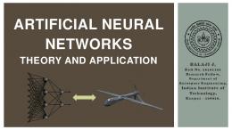
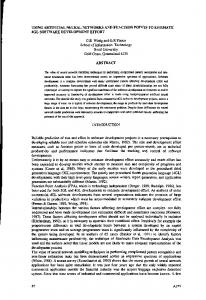
3 between intervals [𝑎𝑖 , 𝑏𝑖 ] and [𝑎𝑖+1 , 𝑏𝑖+1 ] determines whether the level sets 𝑋𝑖 and 𝑋𝑖+1 will have nonempty intersection, which in turn determines the number of edges in the graph. When the intervals [𝑎𝑖 , 𝑏𝑖 ] all have the same length 𝑅 and the intersection of every pair of adjacent intervals also has the same length 𝑟, the percent overlap is said to be (𝑟/𝑅)%. More generally, for a function ℎ : 𝑋 → R𝑛 , the Mapper method constructs a topological space called a simplicial complex, of which a graph is a one-dimensional example. In its full generality, the Mapper method applied to a function ℎ : 𝑋 → R𝑛 results in a simplicial complex with one vertex (or 0-simplex) for every cluster, one edge (or 1simplex) connecting a pair of vertices whenever 2 clusters from neighboring level sets have nonempty intersection, one triangular face (or 2-simplex) filling the region enclosed by three edges whenever 3 clusters from neighboring level sets have nonempty intersection, one solid tetrahedron (or 3simplex) filling the region enclosed by four triangles whenever 4 clusters from neighboring level sets have nonempty intersection, and so on. The level sets, and thus the simplicial complex, are determined by the size and shape of the regions used to cover the image of ℎ. There are several common ways to cover bounded regions in R𝑛 , such as using rectangles, hexagons, or circular disks in R2 or boxes or spherical balls in R3 , and different coverings of the image of ℎ will result in different level sets and thus a different simplicial complex. More details on using the Mapper method to produce a simplicial complex from a function ℎ : 𝑋 → R𝑛 with 𝑛 > 1 can be found in the paper by Singh et al. [5]. An example of the Mapper method is given in Figure 1. In this example, the data set 𝑋 ⊂ R2 is a finite set of points randomly selected on an annulus and the function ℎ : 𝑋 → R is the height projection ℎ(𝑥, 𝑦) = 𝑦. Singlelinkage clustering was used on each of the ℓ = 3 level sets 𝑋1 = ℎ−1 ([−2, 0]), 𝑋2 = ℎ−1 ([−1, 1]), and 𝑋3 = ℎ−1 ([0, 2]) which arise from intervals [−2, 0], [−1, 1], and [0, 2] with 50% overlap between neighboring intervals. The level set 𝑋2 is a disjoint union of two sets 𝑋2,1 and 𝑋2,2 which have points with negative and positive 𝑥-coordinates, respectively. Using single-linkage clustering, each of the sets 𝑋1 , 𝑋2,1 , 𝑋2,2 , and 𝑋3 produces one cluster and thus one vertex in the Mapper model, while each of the nonempty intersections 𝑋1 ∩ 𝑋2,1 , 𝑋1 ∩ 𝑋2,2 , 𝑋2,1 ∩ 𝑋3 , and 𝑋2,2 ∩ 𝑋3 produces one edge in the Mapper model.
3. Methods This section provides a description of the Miller-Reaven diabetes study data, how the data will be analyzed using PCA, the configuration of the neural network, and how the Mapper method will be used to visualize the results. 3.1. Case Study: The Miller-Reaven Diabetes Data. In [13, 14, 26], Reaven and Miller describe the results obtained by applying the projection pursuit method to data obtained from a diabetes study conducted at the Stanford Clinical Research Center. The diabetes study data consisted of the (1) relative weight, (2) fasting plasma glucose, (3) area under the
4
Advances in Artificial Neural Systems
2
X
2
X1
2
X2
2
X3
2
X1 ∩ X2
2
1
1
1
1
1
1
0
0
0
0
0
0
−1
−1
−1
−1
−1
−2 −2 −1 0
−2 −2 −1 0
−2
−2
−2 −2 −1 0
(a)
1
2
1
2
−2 −1 0
1
(b)
2
−2 −1 0
1
2
X2 ∩ X3
−1
1
−2 −2 −1 0 2
1
2
(c)
Figure 1: Illustration of the Mapper method applied points on an annulus with ℎ(𝑥, 𝑦) = 𝑦, single-linkage clustering, and ℓ = 3 level sets. Top row: (a) the annular data set, (b) its level sets, and (c) intersections of adjacent, overlapping level sets. Bottom row: (a) the topological model produced by Mapper, (b) its vertices showing clusters in level sets, and (c) its edges showing adjacent level sets that intersect nontrivially.
plasma glucose curve for the three-hour glucose tolerance test (OGTT), (4) area under the plasma insulin curve for the OGTT, (5) and steady state plasma glucose response (SSPG) for 145 volunteers for a study of the etiology of diabetes [27]. The goal of the study was to determine the connection between this set of 5 variables and whether patients were classified as overt diabetic, chemical diabetic, or not diabetic. In the study, 33 patients were diagnosed as overt diabetic, 36 as chemical diabetic, and 76 as not diabetic on the basis of their oral glucose tolerance [13]. 3.2. Principal Component Analysis. To establish a basis for comparison, the Miller-Reaven diabetes study data will be analyzed using principal component analysis (PCA) to project the data from R5 to R3 . PCA is a variance maximizing projection of the data onto a set of orthonormal basis vectors [28–30]. As PCA is a linear projection, some of the lower variance content of the data will be lost when the dimensionality of the data is reduced. Also, since PCA identifies vectors along which the variance (or spread) of the data is greatest, it is sensitive to outliers. 3.3. Neural Networks and Mapper. The general method for analyzing the Miller-Reaven diabetes study data with a neural network and Mapper is as follows. (1) Preprocess the data set and divide it into stratified training and testing sets. If necessary, preprocess the data to reduce noise. (2) Use the training data to construct a neural network ℎ : R𝑚 → R, meanwhile evaluating the error of the neural network on the testing set to prevent overlearning and overfitting. (3) Apply the Mapper method (see Section 2.2) to the neural network function ℎ to produce a diagram of the clusters formed by the neural network. First, the Miller-Reaven diabetes study data were preprocessed by normalizing each of the five data inputs by
finding 𝑧-scores. Since this normalization is an invertible affine transformation, it has no effect on the neural network’s ability to solve the classification problem. The target output values for the neural network were set to −1 for overt diabetic, 0 for chemical diabetic, and 1 for not diabetic. A generalizable neural network was constructed by using 67% of the data for training and holding out 33% for testing, and these sets were stratified so that each class (overt, chemical, and not diabetic) appeared in the same proportion as in the entire data set. No extra measures were deemed necessary to denoise the MillerReaven data set before constructing a neural network. Second, a feedforward, multilayer perceptron neural network was constructed with 5 input nodes, 4 hidden nodes, and 1 output node, and the method of backpropagation via gradient descent was used for weight updates. Many different numbers of hidden nodes were considered, and four hidden nodes were chosen by using mean square error on the training and testing sets as a criterion for determining whether a neural network underfits or overfits the data. The activation functions chosen were 𝑓1 (𝑥) = tanh(𝑥) = (𝑒𝑥 − 𝑒−𝑥 )/(𝑒𝑥 + 𝑒−𝑥 ) and 𝑓2 (𝑥) = 𝑥. The weights and biases in the neural network were initialized by random values between −0.5 and 0.5. This study emphasizes visualizing how the clusters in a neural network evolve during the weight update process. Thus, a learning rate of 0.1 was chosen to be small so that as the weights and biases were updated, changes in the topological model produced by Mapper could be observed. Neural network performance was evaluated after every cycle through the training data (i.e., epoch). The training data were the same (i.e., not reselected) from epoch to epoch, and they were presented to the neural network in random order to expedite learning [31]. The implementation of the neural network was written by the author in Matlab/Octave and used the standard backpropagation algorithm by stochastic gradient descent [10, Chapter 11]. Finally, the Mapper method (see Section 2.2) was applied to the neural network to produce a cluster diagram of the level sets in the neural network after several different stages of the weight update process during the formation of the neural
Advances in Artificial Neural Systems
5
Table 1: Principal values and their percentages of the total variance in the Miller-Reaven data. Variance in the five PCA directions Variance 2886.6 868.2 330.6 Percent of total variance: 90.54 8.19 1.19 𝜎𝑖2 :
84.4 0.07
0.0 0.00
network. Using Mapper to visualize the clusters in the neural network as the neural network develops shows how the clusters in the neural network change as the training data is learned. Mapper was implemented in Matlab/Octave [32] and utilized GraphViz [33] to produce the graphs. The clustering algorithm used for Mapper was single-linkage clustering. The clusters in the level sets were viewed at different resolutions by varying the number of level sets and the amount of overlap between them. Decreasing the number of level sets can be used to reduce sensitivity to noise. The diagram of clusters in the neural network will be validated by visual comparison to the PCA results.
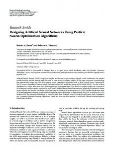
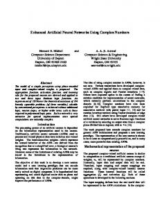
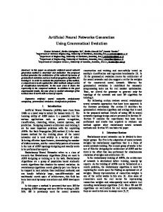
4. Results and Discussion This section describes the results of analyzing the diabetes data using PCA and a neural network. Also, the PCA results are compared to the Mapper cluster diagrams for the neural network. 4.1. Results for Principal Component Analysis. The results of principal component analysis on the Miller-Reaven diabetes study data for dimension reduction from R5 to R3 are shown in Table 1 and Figure 2. The PCA results in R3 show that the data consists of a large central cluster of nondiabetic patients (red +), and that clusters of patients diagnosed as overt diabetic (blue ∘) or chemical diabetic (green ×) emanate away from the large central cluster in two different directions. The PCA results show that the classification problem is not entirely linearly separable in R2 by two lines, but it suggests that it may be possible to construct two planes in R3 (and thus also in R5 ) that separate the data into three categories with a small number of misclassified patients. The PCA results suggest that a neural network which uses a moderate number of separating hyperplanes (i.e., a neural network with one hidden layer and a moderate number of hidden nodes) might be able to solve this classification problem completely. The projections of the PCA results to R2 shown in Figure 2 show that from left to right there is a progression of diagnoses from not diabetic (red +) to chemical diabetic (green ×) to overt diabetic (blue ∘). The principal values in Table 1 show that almost all of the total variance in the data is captured by the first two principal components, which suggests that the original data set in R5 could be projected to R2 , as in Figure 2, thereby effectively compressing the data in the three directions in which it has very little variance. 4.2. Results for a Neural Network with Mapper. The performance of the neural network during the weight update process is given in Figure 3. The number of patients misclassified
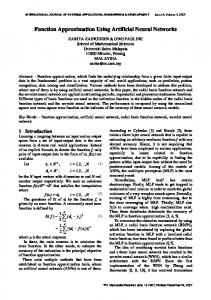
is determined by rounding the output of the neural network to the nearest integer and then counting the number of times the rounded outputs differ from the target outputs. These performance results show that the classification problem can be solved by a neural network for the entire data set. Figure 3 shows that the mean square error (MSE) on the testing set is almost always less than on the training set and that MSE on the testing set rarely increased while the MSE on the training set decreased, which indicates that the neural network did not overlearn the training set. The spikes in Figure 3 likely occur because different classes of input points are very close to each other, and thus small changes in decision boundaries (i.e., separating hyperplanes) for the neural network could lead to sudden changes in the amount of error. The positive performance results in Figure 3 after epochs 12, 32, 57, and 107 indicate four interesting neural networks which misclassified 7, 2, 2, and 0 patients. The neural network after epoch 12 would be a good choice for a compromise between performance and training time since it had a small number of misclassifications and it trained in only a few epochs. The neural network at epoch 12 had an observed success rate of 138/145 = 95.17%, and thus with 95% confidence the true success rate is between 90.37% and 97.64%. It should be noted that the data set is relatively small, so the true success rate of the resulting neural network has a somewhat large confidence interval. The results for using ℓ = 3 and ℓ = 10 intervals (i.e., level sets) in Mapper are shown in Figures 4 and 5, respectively. These results show how the cluster diagrams in the neural network evolve as the number of weight updates increases. The color of each node (i.e., vertex) indicates the average neural network output value of all of the points in that node. Output values of the neural network are encoded using a color gradient in which dark blue indicates values near −1 (overt diabetic), light blue/green indicates values near 0 (chemical diabetic), and dark red indicates values near 1 (not diabetic). The size of each node is proportional to the number of patients in that cluster, and the number in each node is the number of patients in that cluster. Note that the results in Figures 4 and 5 are free-form cluster diagrams in the sense that the absolute position of each node is not important, but the adjacency of nodes connected by edges is important. Further, chains of nodes connected by edges reveal a partial ordering given by the neural network to patients in different nodes, who are assigned different output values by the neural network. 4.3. Discussion. The Mapper results in Figures 4 and 5 show that the graph is connected until the error becomes very low, at which point it may split into several connected components. With only three level sets and 25% overlap of intervals in Figure 4, there are only a few clusters in the neural network and they each have a large number of patients. In contrast, using ten intervals and 50% overlap in Figure 5 produces a higher resolution picture that displays chains of vertices linked by edges for much of the evolution of the neural network. The chains of vertices in Figures 4 and 5 progress from red (not diabetic) to green (chemical diabetic) to blue (overt diabetic), just as the PCA results in R2 do in Figure 2. The large clusters in Figure 5 are useful because they identify homogeneous groups of patients who
6
Advances in Artificial Neural Systems Principal component analysis on Miller-Reaven data
Principal component analysis on Miller-Reaven data (top view) 200
0 200 100 0 −100
Principal component analysis on Miller-Reaven data (side view)
100
−200
0
0
500
0 −200 −400
1000
−400
−100
0
500
1000
0
500
1000
Neural network performance
0.2 0.15 0.1 0.05
Misclassified patients
Mean square error
Figure 2: Principal component analysis of the Miller-Reaven diabetes data. The diagnosis is color coded with a red + for not diabetic, a green × for chemical diabetic, and a blue ∘ for overt diabetic.
0
0
20
40
60
80
100
0
20
40
60 Epoch
80
100
25 20 15 10 5 0
Training Testing
Figure 3: Neural network performance measurements.
have similar test results and similar diabetes classification by the neural network. When several clusters are joined together in a linear chain, the ordering of the vertices in the chain tells about the distribution of patients in a linear ordering. Larger clusters in a chain, as in Figure 5, indicate large groups of patients whose diabetes type is readily classified, whereas smaller clusters in a chain indicate patients who are closer to transitioning from one diabetes type to another. Singleton clusters in Figure 5 that are attached to a larger cluster on a chain indicate individual patients that are on the periphery of a larger cluster. The prominent Y shape in the neural network at epoch 57 in Figure 5 has two distinct blue chains at the top of the Y that result from the sparse blue points in the top view and side view of the PCA analysis in Figure 2. The red barbell shaped singleton cluster in Figure 5 occurred because the value assigned to that one outlier patient by the neural network happened to lie at the intersection of two level sets. In the neural network at epoch 107, the clustering problem has been solved with zero misclassified patients, which means that the level sets ℎ−1 ([−1.5, −0.5]), ℎ−1 ([−0.5, 0.5]), and
ℎ−1 ([0.5, 1.5]) are disjoint and have 33, 36, and 76 patients, respectively. The reason why the neural network at epoch 107 in Figure 4 is connected, rather than disjoint, is that the range of the neural network is [−1.24, 1.15], and thus with 25% interval overlap, the figure shows the level sets ℎ−1 ([−1.24, −0.28]), ℎ−1 ([−0.52, 0.43]), and ℎ−1 ([0.20, 1.15]), which have nonempty intersections and contain 38, 35, and 82 patients, respectively. Using projection pursuit instead of PCA in [13, 14], Miller and Reaven showed that in R3 this diabetes data looks like a central cluster of nondiabetic patients with two different “flares” of clusters of overt and chemical diabetic patients emanating from this central cluster, which is very similar to the PCA results in Figure 2. This is not surprising since PCA can be viewed as an example of projection pursuit [29]. Further, analysis of the Miller-Reaven data using Mapper with a kernel density estimator in [5], instead of a neural network, also produced a topological model for the data with a central cluster and two “flares” analogous to the projection pursuit results. Examination of the PCA results suggests that while a kernel density estimator might work well for overall shape, it might not be very accurate in differentiating between red (non-diabetic) and green (chemical diabetic) in Figure 2 because they are interspersed to some extent. Viewing the projection pursuit and PCA results in R3 shown in Figure 2 as a central cluster with flares, it would appear that the green (chemical diabetic) is connected to red (not diabetic) which is connected to blue (overt diabetic). However, viewing the PCA results in R2 shown in Figure 2 suggests that the clusters should be connected to each other in the order red to green to blue, as the neural network has done in many of the cluster diagrams in Figures 4 and 5. According to Halkidi et al. [34], visualization of a data set is crucial for verifying clustering results. The PCA results in Table 1 indicate that the inputs in R5 can be projected to R2 without much variance being lost, so the data is very close to being two-dimensional. Further, the results of projecting the data to R2 shown in Figure 2 make this data set ideal for the purpose of validating a clustering method by visual comparison. The neural network performance results in Figure 3 show that the neural network was able to solve the MillerReaven diabetes classification problem. Visual comparison of
Advances in Artificial Neural Systems
36
44
84
7
31
43
(a)
86
36
38
(b)
35
83
82
38
(c)
(d)
Figure 4: Mapper visualization of clusters in the neural network for the Miller-Reaven diabetes study data using 3 intervals with 25% overlap. From left to right: clusters in the neural network after 12, 32, 57, and 107 epochs. The neural network classification is color coded with dark blue for overt diabetic (class −1), light blue/green for chemical diabetic (class 0), and dark red for not diabetic (class 1).
1
31
30
6
6
9 1 16
1
1 13
30 1
2
1 (a)
2
15 25
1
1 1
10
12 14
18
68 72
68
(b)
1
7
12
15 1
1
10
17
13 1
33
1 23
23
14 65
2
15
18
5
2
12
1
17
25
2
2
10 13
1
1
1 (c)
(d)
Figure 5: Mapper visualization of clusters in the neural network for the Miller-Reaven diabetes study data using 10 intervals with 50% overlap. From left to right: clusters in the neural network after 12, 32, 57, and 107 epochs. The neural network classification is color coded with dark blue for overt diabetic (class −1), light blue/green for chemical diabetic (class 0), and dark red for not diabetic (class 1).
the neural network and Mapper results in Figures 4 and 5 with the PCA results in Figure 2 reveal that the cluster diagram and PCA results convey the same information in compressed (i.e., clustered) and noncompressed ways, respectively. Thus, these results serve to validate the cluster diagrams generated by a neural network and Mapper.
5. Conclusions Neural networks and the Mapper method have a symbiotic relationship for solving clustering problems and modeling the solution. The level sets of a neural network can be used to solve a clustering problem for high-dimensional data sets, and the Mapper method can produce a low-dimensional cluster diagram from these level sets that shows how they are glued together to form a skeletal picture of the data set. Using neural networks and the Mapper method together simultaneously solves the problem that visualizing the level sets of a neural network is difficult for high-dimensional data and the problem that the Mapper method only produces useful results when applied to a function that solves a clustering problem effectively. Together, they combine the efficacy of neural networks at solving clustering problems
with the clarity and simplicity of cluster diagrams produced by the Mapper method, thereby making the neural network’s solution to the clustering problem much easier to interpret and understand. Further, the Mapper method allows the neural network’s solution to a clustering problem to be viewed at different resolutions, which can help with developing a model that shows important features at the right scale. The results of the case study provide evidence in support of the conclusion that using a neural network to solve a clustering problem and the Mapper method to produce a clustering diagram is a valid means of producing an accurate low-dimensional topological model for a data set. In particular, the most important pattern observed in the scatterplot of the PCA results, which was progression classifications from non-diabetic (red +) to chemical diabetic (green ×) to overt diabetic (blue ∘) in Figure 2, was also observed at a finer resolution in the cluster diagram for the neural network in Figure 5. Further, the linear chains of nodes connected by edges in the clustering diagrams in Figures 4 and 5 provided a partial ordering on the neural network results that made the results easier to interpret. In order to firmly establish the validity of using a neural network with Mapper for a wide variety of applications, it is evident that in the future this
8 method should be compared to data analysis methods other than PCA and that further case studies should be done for different types of data sets.
Acknowledgments The author would like to thank Dr. David Housman (Goshen College) and Dr. Nancy Neudauer (Pacific University) for organizing the Research in Applied Mathematics session at the Mathematical Association of America’s MathFest 2012, where preliminary results of this research were presented.
References [1] G. Carlsson, “Topology and data,” Bulletin of the American Mathematical Society, vol. 46, no. 2, pp. 255–308, 2009. [2] H. Edelsbrunner and J. Harer, Computational Topology: An Introduction, American Mathematical Society, Providence, RI, USA, 2010. [3] A. Zomorodian, Topology for Computing, Cambridge University Press, New York, NY, USA, 2005. [4] P. Y. Lum, G. Singh, A. Lehman et al., “Extracting insights from the shape of complex data using topology,” Scientific Reports, vol. 3, article 1236, 2013. [5] G. Singh, F. M´emoli, and G. Carlsson, “Topological methods for the analysis of high dimensional data sets and 3D object recognition,” in Eurographics Symposium on Point-Based Graphics (Prague ’07), pp. 91–100. [6] H. Adams, A. Atanasov, and G. Carlsson, “Morse theory in topological dataanalysis,” http://arxiv.org/abs/1112.1993. [7] C. Marzban and U. Yurtsever, “Baby morse theory in data analysis,” in Proceedings of the Workshop on Knowledge Discovery, Modeling and Simulation (KDMS ’11), pp. 15–21, August 2011. [8] K.-L. Du, “Clustering: a neural network approach,” Neural Networks, vol. 23, no. 1, pp. 89–107, 2010. [9] J. Herrero, A. Valencia, and J. Dopazo, “A hierarchical unsupervised growing neural network for clustering gene expression patterns,” Bioinformatics, vol. 17, no. 2, pp. 126–136, 2001. [10] M. Hagan, H. Demuth, and M. Beale, Neural Network Design, PWS Publishing, Boston, Mass, USA, 1995. [11] R. Marks and R. Reed, Neural Smithing: Supervised Learning in Feedforward Artificial Neural Networks, Denver, Bradford, UK, 1999. [12] R. Rojas, Neural Networks: A Systematic Introduction, Springer, New York, NY, USA, 1996. [13] G. M. Reaven and R. G. Miller, “An attempt to define the nature of chemical diabetes using a multidimensional analysis,” Diabetologia, vol. 16, no. 1, pp. 17–24, 1979. [14] R. Miller, “Discussion—projection pursuit,” Annals of Statistics, vol. 13, no. 2, pp. 510–513, 1985. [15] S. Walczak, “Methodological triangulation using neural networks for business research,” Advances in Artificial Neural Systems, vol. 2012, Article ID 517234, 12 pages, 2012. [16] M. Nicolau, A. J. Levine, and G. Carlsson, “Topology based data analysis identifies a subgroup of breast cancers with a unique mutational profile and excellent survival,” Proceedings of the National Academy of Sciences of the United States of America, vol. 108, no. 17, pp. 7265–7270, 2011. [17] G. R. Bowman, X. Huang, Y. Yao et al., “Structural insight into RNA hairpin folding intermediates,” Journal of the American Chemical Society, vol. 130, no. 30, pp. 9676–9678, 2008.
Advances in Artificial Neural Systems [18] J. Mao and A. K. Jain, “Artificial neural networks for feature extraction and multivariate data projection,” IEEE Transactions on Neural Networks, vol. 6, no. 2, pp. 296–317, 1995. [19] M. A. Kramer, “Nonlinear principal component analysis using autoassociative neural networks,” AIChE Journal, vol. 37, no. 2, pp. 233–243, 1991. [20] D. De Ridder and R. P. W. Duin, “Sammon’s mapping using neural networks: a comparison,” Pattern Recognition Letters, vol. 18, no. 11-13, pp. 1307–1316, 1997. [21] D. K. Agrafiotis and V. S. Lobanov, “Nonlinear mapping networks,” Journal of Chemical Information and Computer Sciences, vol. 40, no. 6, pp. 1356–1362, 2000. [22] W. Pedrycz, “Conditional fuzzy clustering in the design of radial basis function neural networks,” IEEE Transactions on Neural Networks, vol. 9, no. 4, pp. 601–612, 1998. [23] G. Cybenko, “Approximation by superpositions of a sigmoidal function,” Mathematics of Control, Signals, and Systems, vol. 2, no. 4, pp. 303–314, 1989. [24] K. Hornik, M. Stinchcombe, and H. White, “Multilayer feedforward networks are universal approximators,” Neural Networks, vol. 2, no. 5, pp. 359–366, 1989. [25] P. G. Goerss and J. F. Jardine, Simplicial Homotopy Theory, Birkh¨auser, Basel, Switzerland, 2009. [26] P. J. Huber, “Projection pursuit,” The Annals of Statistics, vol. 13, no. 2, pp. 435–475, 1985. [27] D. F. Andrews and A. M. Herzberg, Data: A Collection of Problems from Many Fields for the Student and Research Worker, Springer, New York, NY, USA, 1985. [28] C. R. Rao, “The use and interpretation of principal component analysis in applied research,” Sankhya Series A, vol. 26, pp. 329– 358, 1964. [29] R. J. Bolton and W. J. Krzanowski, “A characterization of principal components for projection pursuit,” The American Statistician, vol. 53, no. 2, pp. 108–109, 1999. [30] C. Croux, P. Filzmoser, and M. R. Oliveira, “Algorithms for Projection-Pursuit robust principal component analysis,” Chemometrics and Intelligent Laboratory Systems, vol. 87, no. 2, pp. 218–225, 2007. [31] Y. LeCun, L. Bottou, G. Orr, and K. M¨uller, “Efficient backprop,” in Neural Networks: Tricks of the Trade, Springer, New York, NY, USA, 1998. [32] D. M¨ullner and G. Singh, “Mapper 1d for matlab,” 2013, http://comptop.stanford.edu/programs/. [33] “Graphviz—graph visualization software,” 2013, http://www .graphviz.org/. [34] M. Halkidi, Y. Batistakis, and M. Vazirgiannis, “On clustering validation techniques,” Journal of Intelligent Information Systems, vol. 17, no. 2-3, pp. 107–145, 2001.
Journal of
Advances in
Industrial Engineering
Multimedia
Hindawi Publishing Corporation http://www.hindawi.com
The Scientific World Journal Volume 2014
Hindawi Publishing Corporation http://www.hindawi.com
Volume 2014
Applied Computational Intelligence and Soft Computing
International Journal of
Distributed Sensor Networks Hindawi Publishing Corporation http://www.hindawi.com
Volume 2014
Hindawi Publishing Corporation http://www.hindawi.com
Volume 2014
Hindawi Publishing Corporation http://www.hindawi.com
Volume 2014
Advances in
Fuzzy Systems Modelling & Simulation in Engineering Hindawi Publishing Corporation http://www.hindawi.com
Hindawi Publishing Corporation http://www.hindawi.com
Volume 2014
Volume 2014
Submit your manuscripts at http://www.hindawi.com
Journal of
Computer Networks and Communications
Advances in
Artificial Intelligence Hindawi Publishing Corporation http://www.hindawi.com
Hindawi Publishing Corporation http://www.hindawi.com
Volume 2014
International Journal of
Biomedical Imaging
Volume 2014
Advances in
Artificial Neural Systems
International Journal of
Computer Engineering
Computer Games Technology
Hindawi Publishing Corporation http://www.hindawi.com
Hindawi Publishing Corporation http://www.hindawi.com
Advances in
Volume 2014
Advances in
Software Engineering Volume 2014
Hindawi Publishing Corporation http://www.hindawi.com
Volume 2014
Hindawi Publishing Corporation http://www.hindawi.com
Volume 2014
Hindawi Publishing Corporation http://www.hindawi.com
Volume 2014
International Journal of
Reconfigurable Computing
Robotics Hindawi Publishing Corporation http://www.hindawi.com
Computational Intelligence and Neuroscience
Advances in
Human-Computer Interaction
Journal of
Volume 2014
Hindawi Publishing Corporation http://www.hindawi.com
Volume 2014
Hindawi Publishing Corporation http://www.hindawi.com
Journal of
Electrical and Computer Engineering Volume 2014
Hindawi Publishing Corporation http://www.hindawi.com
Volume 2014
Hindawi Publishing Corporation http://www.hindawi.com
Volume 2014