âofficeâ, or âJoe's houseâ. The data was .... [6] Jain, R., Lelescu, D., & Balakrishnan, M. Model T: an empirical model for ... [13] R.W. Reeder, P. Pirolli, & S. Card.
Dartmouth – Computer Science – Technical Report – TR2006-580
Visualizing Paths in Context Fabio Pellacini Dartmouth College
Lori Lorigo Cornell University
ABSTRACT Data about movement through a space is increasingly becoming available for capture and analysis. In many applications, this data is captured or modeled as transitions between a small number of areas of interests, or a finite set of states, and these transitions constitute paths in the space. Similarities and differences between paths are of great importance to such analyses, but can be difficult to assess. In this work we present a visualization approach for representing paths in context, where individual paths can be compared to other paths or to a group of paths. Our approach summarizes path behavior using a simple circular layout, including information about state and transition likelihood using Markov random models, together with information about specific path and state behavior. The layout avoids line crossovers entirely, making it easy to observe patterns while reducing visual clutter. In our tool, paths can either be compared in their natural sequence or by aligning multiple paths using Multiple Sequence Alignment, which can better highlight path similarities. We applied our technique to eye tracking data and cell phone tower data used to capture human movement. CR Categories and Subject Descriptors: H.5.3 [Information Interfaces and Presentation]: User Interfaces Additional Keywords: Information Visualization, Social Visualization, Time Series Data, Data Stream Visualization 1
Geri Gay
INTRODUCTION
In a growing number of applications, data is captured or modeled as transitions between a small number of areas of interest, considered as a finite set of states. These transitions constitute paths in some space. Examples of such data range from cell phone tower usage to GPS tracking of humans or animals to wireless network activity to eye movements across a screen. The paths also may consist of semantic rather than physical locationbased state sequences. In much of this data, the state space is small and the paths are generally relatively short. It is the transitions of the paths themselves that are important, since they can help scientists discover movement or usage patterns, or even make predictions about next steps at a given point in a path. Markov random models in the form of transition probability matrices have been used to describe the path transitions [6]. However, without the help of visualization and means for path comparison, the paths are often not well understood. While the number of possible states may be small in this class of data, it remains difficult to visualize even a single path, let alone multiple paths, because visits to each state may be frequent, and hence visualization of collections of these paths remains a challenge. Furthermore, a possible solution of finding a representative path for a given cluster can be either misleading or an oversimplification for the data (resulting in data loss or nonrealistic paths), particularly when there is variability. In this work, we introduce a simple circular layout for visualizing these paths with three major benefits. (1) Line crossings are avoided entirely to reduce visual clutter or confusion that can be otherwise introduced even when viewing a single path, which may have many repeat visits and jumps. (2) Two paths can
Cornell University
be compared either in their natural sequences or in an optimally aligned pairing. The latter relies on multiple sequence alignment and can give a more accurate account of paths’ similarities, helping to understand how paths are related. (3) A path can be compared to a group of paths, revealing that path’s similarities or dissimilarities with respect to an entire collection. Markov random models assist in showing a collection’s overall behavior together with an individual path. Our layout design decisions, along with our results from two path datasets are described next, following related work. Both of these datasets are from domains where the analysis of paths and their transitions is important. The first includes a series of eye gaze paths on a web page, gathered using an eye tracker, and the second describes human movement captured from cell phone towers. We then conclude with a summary of our contributions, including limitations of our layout as well as natural extensions. 2
RELATED WORK
Over time, visualization techniques have demonstrated their success at revealing patterns and portraying aggregate information efficiently, such as with large data sets. Flow maps [12], have been used for over a century, and can be very effective when displaying data with a from-to relationship, such as migration, traffic and trade data. Physical locations are typically associated with flow data, and aggregate behavior is desired. In the class of data we are targeting, however, the states may have only abstract locations, and the paths often includes repeat visits and cycles. In particular, the order of the transitions are important in our data, and aggregating paths in the same manner as flow would lose this valuable information. Animation is another visualization method that conveys information about sequential data. Animation has been used to visualize paths, software and algorithms [8]. While animation displays sequential movements intuitively, it becomes increasingly difficult for viewers to place their attention on multiple paths, or on additional valuable contextual information, such as we desire. Hence, for our task we use a still image visualization, while making the path progression clear from start to finish. Since our target data can be represented as transitions between a finite set of states, we also note work on visualizing state transition systems by van Ham et. al. [14]. Their work, however, was designed for large state spaces where the state machine itself is of primary interest, such as program code. Instead, our work visualizes collections of paths and makes it easy to find similar paths, or path to group similarities and differences. Lastly, our circular layout framework described below is somewhat similar in design to popular radial layouts [5]. Those layouts have been used for tree-like hierarchical networks, placing a root node at the circle’s center, branching outward to the node’s children in concentric circles [15]. Since our target data consists of paths, rather than hierarchical data, it naturally follows that our use of the concentric circles differs; in our design, the concentric circles represent points in the path rather than hierarchies in the network. Furthermore, transitions and path prediction is important to our data domains, so circles are also used to indicate transition and state likelihoods.
Dartmouth – Computer Science – Technical Report – TR2006-580
Figure 1. Linear (left) and circular (right) layout.
3
LAYOUT DESIGN
As stated, our goal in this work is to display paths in context. Displaying paths involves displaying an ordered sequence of states, with transitions between them. At each state, additional information may be desirable, such as time spent, depending on the dataset of interest. Displaying paths in context involves displaying a path with respect to some surrounding data or information. In this work, we provide for the displaying of a path as compared to (1) another path, and (2) a group of paths. We discuss our approach towards each of these tasks in detail below. Each of paths in the examples in this section was taken from the eye tracking dataset. 3.1 Displaying Paths When designing a display for paths, we were interested in making the path behavior clearly visible, including direction and state specific information, and allowing for integration of the path display with additional contextual information, discussed later. We also leveraged traits of the kind of data we are proposing to illustrate, particularly, paths with a small number of areas of interest, that are generally relatively short in length. Even for our target data class, straightforward graph layout algorithms in which nodes are the states and edges are the state transitions, result in unclear path behavior, due in part to line crossings, but also because paths frequently revisit locations, contain cycles, or fluctuate between pairs of states. The confusion only intensifies if more than one path is placed on the graph. Possible solutions of using color or edge markings to help the viewer see the paths are inadequate in these cases. We considered two alternative displays, a linear layout and a circular layout, shown in Figure 1 using the same path. In these examples, there are 10 states, labeled A through L. The linear layout is simply a 2 dimensional grid, placing the states, or areas of interest, on the vertical axis and plotting the path along the x axis, so that the path is viewed left to right. This layout is suggestive of a timeline, even though the sequences may or may not be modeled according to time. The circular layout arranges the states in a circle and utilizes a series of concentric circles emanating outward from the circle of states. These concentric circles serve as the “timeline” for the path, with the first state in the path starting closest to the center (state C). In both layouts, the
ordering and placement of the states affects the look of the path; this ordering can either be arbitrary, determined by the data, or chosen to minimize long distance transitions. While we hoped that the simpler linear grid would suffice, we found that the circular layout was superior. In that layout, it was easier to follow the state labels, and see patterns such as state fluctuations, or paths that span many states. Also, information about the group of paths, described later in 3.2.3 (shown by the differently sized circles near the state labels), is easy to follow while still keeping gaze on the single path for comparison. Lastly, the circular layout is less sensitive to long jumps, as seen in the center of the linear layout, requiring at most ½ the circumference to connect any two states. 3.1.1 Activity vs. Time-Centered Display In many domains, activity-centered displays of the paths are more interesting than time-centered displays. We distinguish activity-centered paths as those which highlight the state sequence alone, without respect to what state the path was in at a given time along the path. To illustrate this, we place steps along the path, which we call satellites, in the same concentric circle, rather than moving outward in the circle, if the state did not change. This also makes the path more manageable, particularly when it is long, and highlights repeated presence in a state. Figure 2, taken from the path above, shows a case where the path repeatedly visited state F in the sequence, marked by several satellites in a row.
Figure 2. Activity-centered repeat satellites.
Dartmouth – Computer Science – Technical Report – TR2006-580 Satellite darkness is used to show additional information about a visit to a state, such as time spent in the state in these examples. In the sample above, the subject rarely spent a relatively long time in any step on the path, noted by a dark black satellite. Edge darkness can be used to convey the length of a subsequence in a given path, connoting spanning behavior. In this example, if the number of states is at least 3 (the sequence doesn’t bounce back), the edge is dark. If it is desirable to show even additional information about each step in the path one can use selection (mouse click on a satellite) and display relevant values in the very center of the circle, or in an additional viewing area. 3.2 Paths in Context Our simple path layout was intentionally designed to allow for integration with additional visual components in order to describe the path’s context. Context is important for analysis of a path with respect to other path behavior or path group behavior. While paths can readily be compared according to numeric properties such as their lengths, number of states visited, or their average time spent in states, it remains challenging to compare are the transitions which shape the path as a whole. It is these transitions that allow us to make predictions, or to find common subpaths in the data. How can we visualize a path’s shape as compared with another path or a collection of paths? 3.2.1 Path to Path Comparison In our layout, we allow both the direct comparison of two paths, for which plot the paths as “mirror images”, and the ability to view a single path in the context of a second path, keeping the first path in the forefront, while highlighting the path to path similarities. Plotting multiple paths in the same space quickly causes clutter and confusion, so we adopted these alternatives. In each case, we can display the paths either in their original form, or by first aligning them, using pairwise sequence alignment [11], or in the case of groups of paths, multiple sequence alignment [1]. The aligned form helps to better reflect similarities, while the natural form remains important for time-dependent data. To align paths, we minimize the number of state insertions, deletions, or substitutions needed to transform one path into the other. That number is also known as the Levenshtein distance [4, 7] and has been used in quantitative analysis of eye tracking scanpaths [5]. For instance, path ABCDEF is paired with path BCDEFA as in its original and aligned form. ABCDEF ABCDEF – BCDEFA –BCDEFA These paths are in fact similar, and have a Levenshtein distance of two. However, in their natural form, no states line up. Figure 3 and 4 illustrate a path in the context of a second path, using the natural and aligned pairings. Here, dark satellites and edges represent state and transition agreement. In our layout, we also detect where insertions would have occurred according to the alignment and place a connecting line. Notice, the alignment finds more similarity, recognizing paths similar in shape, given a small number of insertions or deletions. In order to view the entire second path, rather than only its similarities, Figure 5 shows the paths in the mirror format. Symmetry is easily recognizable, and even a quick glance shows the paths’ overall similarity. 3.2.2 Graphical User Interface Operation Our graphical user interface for selecting the paths was also designed to make it very easy to find similar paths, since once a path is selected, the paths are ordered according to their distance from that path, so the user can very quickly browse through the paths in order of their similarity. The user can select alignment or no alignment, and can select between activity or time centered displays. Selection for groups of paths is also available.
Figure 3. Unaligned path to path similarities.
Figure 4. Aligned path to path similarites.
Figure 5. Aligned path to path mirror image comparison.
Dartmouth – Computer Science – Technical Report – TR2006-580 3.2.3 Path to Group Comparison The central area of the layout, shown in Figure 6 contains the states and labels, and provides information about overall group behavior that can be used as a guide while viewing a path. First, the size of each state is proportional to the number of visits to that state over the entire collection of paths. Next, inside each state, we place circles whose size represents the likelihood of transitions to the respective states given the current state. For instance, because of the placement of two predominant circles inside state C, we see that it is highly likely one will next jump to either B or D. We capture these transition likelihoods with a first order Markov model describing the collection of paths. Hence, when viewing a step in a path, one can glance to see how popular that state was, and what the most likely next step would have been. Or, since the center will not change for a given data set, one can approximate average behavior from these transition likelihoods.
7 shows the path as compared with the collection. Dark edges indicate that the likelihood of the transition is greater than random in the model, and satellites are darkened to compare the number of satellites in a state with the group average. This allows a user to quickly see which paths either agree or disagree with respect to some group. To select the group, a user can select any number of closest aligned paths, the entire collection, or can use groups defined by the data. For instance, the data may be classified according to gender, age, or other relevant class. 4
RESULTS AND DISCUSSION
Below we discuss our results when applying two different data sets to our tool. 4.1 Eye Tracking Scanpaths The first data set we consider comes from eye tracking capture of subjects’ eye fixations paths while interacting with the Google results page upon performing a Google search query [10]. Eye tracking is an important tool for many usability analysts, psychologists, and other scientists, and eye gaze paths, or scanpaths are of great interest but difficult to analyze [4, 7, 13]. Eye tracking heatmaps [3], for example, show an aggregate of where people looked but cannot show sequential behavior which is important for predicting paths or comparing paths against a control group, for example. In this domain, scanpaths are typically represented as sequences of areas of interests, or states (also called “lookzones”). The ability to map pixel gaze coordinates to areas of interest comes standard with all major eye tracking software. In this dataset, there were 10 areas of interest, one for each of the 10 results returned from a Google query. Hence, the scanpaths revealed the order in which the query result abstracts were viewed. We discarded paths smaller than length 3, leaving 412 paths as input to our tool. 4.1.1
Single Paths
Figure 6. Markov random models and state labeling.
Figure 8. Jumping pattern seen between states B and C.
Figure 7. Path in the context of the collection of paths.
Second, we can highlight when a path agrees with the group behavior, as we did with path to path comparison. We determine this using either the first order Markov model, or alternatively a second order Markov model, as appropriate for the dataset. Figure
Viewing single paths in the Google data set, showed clearly the behavior of the paths, and also surprisingly highlighted a couple of immediate patterns. The first is a jumping pattern, shown in Figure 8 by the repeated edges between states B and C. This clearly visible was quickly discovered to be prevalent in many of the paths. The subject was likely making a decision between the search result abstracts for two different web pages before making a selection, or clicking on one of them. Visualizing the same paths in the linear layout made this discovery less immediate. Second,
Dartmouth – Computer Science – Technical Report – TR2006-580 the act of reading, or repeatedly fixating within a given state was clearly visible, shown by the presence of many satellites clustered together, as along state F in Figure 2. This pattern was noticeable in many of the paths. Such predominant kinds of scanpath behavior were quickly seen while browsing the paths. 4.1.2 Paths in Context Figures 3, 4, and 5 above showed the comparison of a path to another and Figure 7 above showed the same path compared with the transition behavior of the entire data set. While certain paths had high similarity to others, we quickly observed that the path sequences varied considerably across the entire set. In this case, the ability find closest paths and to define or distinguish subgroups was valuable. Also, it shows that it may not make sense to find an “average path” to represent the entire collection, but instead there may be multiple clusters of related paths, for which an average path is more suitable. For this dataset, the ability to view and compare patterns from paths and groups of paths provided an understanding that alternative non-visual approaches could not.
4.2 MIT Reality Mining Data Set Our second data set consists of cell phone tower usage used to approximate human movement, made available by the MIT Reality Mining project [2]. Data about human or even animal movement is more easily captured today, and is important in many areas of research such as sensors, wireless networks, and HCI. This subset we use contains proximity data taken for one subject over 3 months. The mobile phone towers in that data were associated with personally relevant places such as “home”, “office”, or “Joe’s house”. The data was first compressed into half hour intervals using a sliding window, and a representative state for each half hour was chosen. The 10 most visited places served as our areas of interest, or state space in this example. We then extracted a single path for each day, from which we selected those paths whose states all belonged to our state space. These paths constituted roughly 1/3 of the original data. Using our layout, one can quickly view the subject’s movement on a given day, compare that day against another or multiple days, and see the overall behavior for the entire 3 months.
Figure 9. Time-centered path to path comparisons, single (left) and mirror (right) image.
Figure 10. Activity-centered path to path comparisons, single (left) and mirror (right) image.
Dartmouth – Computer Science – Technical Report – TR2006-580 4.2.1 Activity and Time Centered Path Comparison In this data set, it is interesting to consider both activity and time-centered layouts. The activity-centered paths allow a user to compare the general activities that the subject did in a given day as inferred from the semantic locations such as home, office, restaurant, or a person’s house. The time-centered paths instead allow one to compare where a subject was at a given time during the day. Alignment provides a natural way to compare the activity-centered paths, however, it is less appropriate for time centered paths (since resulting insertions and deletions will alter the paths’ timelines). Figures 9 shows the time-centered comparisons of two paths using the circular and mirror displays. In these paths, we see that the subject spent the majority of his time between states A and C, which not surprisingly correspond to home and work, or night and day. Figures 10 shows activitycentered comparisons for another pair of paths. The presence of dark edges and satellites in Figure 10 reveals that there is considerable agreement of path 1 to path 2. Looking at the mirror image shows that agreement while additionally noting the differences. For example, the path on the right spends repeated time in state D while that on the left does so in state C. Our last example, in Figure 11 below, shows the path with respect to the entire collection. The prevalence of transition similarities, again depicted as dark edges, suggests that the day sequence was typical of that of the entire 3 months.
which was shown to be less apparent in the simpler linear layout. In the MIT reality mining data, frequently, paths were well aligned, and anomalous days were easily observed as such in the context of the entire path set. Our GUI made it easy to find similar paths, and recurring patterns. So far, visual cues such as color and size were used conservatively, making the addition of other information possible if it becomes desirable depending on the user or data domain. Note, depending upon preference, color could have easily been used instead of dark edges, or two colors could have highlighted agreement and disagreement in the same manner. Now that we have a layout and tool available, a thoughtful user study would be valuable. We have noted that our design is limited to data with a small number of states, and relatively short paths. The states in our target data also typically have a semantic meaning, and so the state transition behavior is very important in understanding the overall data. We have shown examples of such data, and discussed several ways in which our layout illustrates the important aspects of the state paths and their context. ACKNOWLEDGEMENTS This section removed for blind review. REFERENCES [1] [2] [3] [4] [5]
[6]
[7]
[8]
[9] [10] Figure 11. Path in the context of the entire collection.
5
CONCLUSION
In summary, we have described a simple layout for displaying data that is captured or modelled as paths through a small number of states, or areas of interests, and for which individual paths, and their comparison to others are important. Our layout provides the benefits of clearly visualizing paths, without line crossovers, the flexibility of selecting paths and groups for comparison, and conveys important contextual information using the Markov random models for the paths and Multiple Sequence Alignment. In our sample data sets, paths are clearly visible, as are their similarities with respect to other selected data. The interface itself also assists browsing for similarities by ordering paths according to their distance to a selected path. In our test sets, patterns have already quickly emerged. For example, in the eye tracking collection both jumping and reading behaviors were apparent, and transition likelihoods were clearly shown. Our circular layout assisted in understanding the combined path and group behavior,
[11]
[12]
[13]
[14]
[15]
Bacon, D. J. & Anderson, W. F. (1986) J. Mol. Biol. 191, 153-161. Eagle. N., MIT Reality Mining Project. http://reality.media.mit.edu/ EyeTools, Inc. http://www.eyetools.com/ Hembrooke, H., Fuesner, M., & Gay. Averaging scan patterns and what they might tell us. ETRA, Late Breaking Results, 2006. Herman, I., Melançon, G., and Marshall, M. S., “Graph Visualisation and Navigation in Information Visualisation,” Proc. of Eurographics ’99, Aire-la-Ville, 1999. Jain, R., Lelescu, D., & Balakrishnan, M. Model T: an empirical model for user registration patterns in a campus wireless LAN. Proc. of Mobile Computing and Networking (MobiCom), pages 170-184, Cologne, Germany, August 2005 Josephson & Holmes. M.E. 2002. Visual Attention to Repeated Internet Images: Testing the Scanpath Theory on the World Wide Web, ETRA, 43-49. Kerren, A. & Stasko, J. (2002). "Algorithm Animation Introduction", Software Visualization State of the Art Survey, Springer LNCS 2269, Editor: Stephan Diehl, Chapter 1, pp. 1-15. Levenshtein, see http://en.wikipedia.org/wiki/Edit_distance Lorigo, L., Pan, B., Hembrooke, H., Joachims, T., Granka, L., & Gay, G. The Influence of Task and Gender on Search and Evaluation Behavior Using Google. Information Processing and Management (IPM), 2005. S. Needleman and C. Wunsch. A general method applicable to the search for similarities in the amino acid sequences of two proteins. Journal of Molecular Biology, 48:443--453, 1970. Phan, D., Xiao, L., Yeh, R., Hanrahan, P., & Winograd, T. (2005). Flow Map Layout. In Proc. of the 2005 IEEE Symposium on information Visualization INFOVIS. R.W. Reeder, P. Pirolli, & S. Card. Webeyemapper and weblogger: Tools for analyzing eye tracking data collected in web-use studies. In Proc. of CHI 2001. van Ham, F., van de Wetering, H., & van Wijk, J.J. "Interactive Visualization of State Transition Systems", IEEE Transactions on Visualization and Computer Graphics Vol. 8 No. 4, 2002. Yee, K.-P., Fisher, D., Dhamija, R., Hearst, M. Animated exploration of dynamic graphs with radial layout. Proc. of IEEE Symposium on Information Visualization 2001, IEEE Press, 43 – 50.