Visually Aided Feature Extraction from 3D Range Data - CEC

Visually Aided Feature Extraction from 3D Range Data Chhay Sok, Martin D. Adams School of Electrical & Electronic Engineering, Nanyang Technological University, Singapore {sok,eadams}@ntu.edu.sg

Abstract— Robust feature extraction within 3D environments is a crucial requirement for many autonomous robotic and tracking applications. 3D Laser range finders and cameras provide extremely rich data about an environment. However, the algorithms which attempt to compress the vast data sets produced by these sensors into features, tend to be fragile in the presence of sensor noise, or computationally expensive. This paper presents a 3D feature extraction technique which greatly compresses 3D range data based on principal component analysis (PCA). PCA can provide a greatly compressed vector set, representing the dominant directions of data points, thus grouping them into planes or lines. It is shown however, that the naive application of PCA to full, 3D, point cloud data sets, results in a poor representation of the dominant data directions. Therefore, a combination of a panoramic camera and 3D laser range finder is used to extract robust planes from 3D range data. The panoramic camera image is first filtered with the Mean Shift algorithm to smooth segments within it, whilst preserving the integrity of the segment edges. These segments are then used to guide the PCA, through an approximate image to range space calibration, to act on the corresponding individual segments of range data. The application of PCA to segmented subsets of 3D point cloud data sets, will be shown to be robust for the detection of planes in both indoor and urban, outdoor environments.

I

I NTRODUCTION

3D laser range representations of the environment are now popular, since rich descriptions of an autonomous vehicle’s surroundings can be made available for robust navigation [2]. However, since such 3D scans are composed of dense point clouds, the processing necessary for successful feature extraction can be overwhelming. Horn et al. [5] extracted vertical planes from 3D data, with the aim of aiding autonomous docking procedures, based on planar data association with predicted plane positions. Weingarten et. al. used a segmentation method to decompose the robot navigational space into cells [6]. 3D, laser based, raw data points were associated with their corresponding cells and a recursive region growing algorithm was applied to “grow” the data points into possible planes. Another approach for 3D planar extraction is discussed in [4]. The approach employs the expectation maximization algorithm to fit a planar model to 3D range data. In the presence of Gaussian noise, the goal of the algorithm is to determine the set of planes that maximizes the likelihood of the data. This research is funded in part by the Singapore National Research Foundation through the Singapore - MIT Alliance for Research & Technology Centre for Environmental Sensing & Modelling (CENSAM).

3D planar extraction from a single still image has been examined in [13], in which superpixel segmentation is used to find the 3D position and orientation of the 3D surface it represents. Such information can also be obtained from stereo cameras. In [3], a Digiclops tri-stereo camera is used to provide 3D range information. Grid-based range data segmentation and plane extraction techniques are implemented with the range data. However, it is pointed out that the success of stereo vision is highly dependent on lighting, distance and surface texture conditions. Laser range finders and cameras have been integrated to form fused sensing systems for applications varying from 3D SLAM to vehicle recognition [7]. In this article, both the visual and laser range information are fused under a grid based scheme. Although grid based methods can, over time, reduce the effect of sensor errors in autonomous navigation frameworks, they are accompanied by large computational issues, since at each time step, each grid cell’s occupancy probability value must be recalculated. This paper describes an integrated system which combines a 3D LADAR and panoramic camera. Visual information is obtained from stitched images produced by the panoramic camera and 3D point cloud data is produced by the continuously scanning, 3D laser range finder. It is demonstrated that dominant data directions, based on principal component analysis (PCA), can be used to efficiently compress and represent 3D point cloud subsets of complete 3D laser range scans. The subsets are generated by first smoothing the panoramic camera image, whilst preserving, as far as possible, the image edges. Smoothed regions of approximately constant colour are then segmented to form clusters. Through an approximately calibrated transformation between the 3D laser range point and image pixel locations, the image clusters can be used to extract the corresponding 3D laser point cloud subsets. Applying PCA to these subsets yields robust, planar segments requiring minimal computational storage, which can be used as features within an autonomous navigation framework. The paper is structured as follows. Section II explains the camera and laser range finder system and section III demonstrates the problems of naively applying PCA to complete 3D range scans. Section IV presents the 3D point cloud data, augmented with colour information. This provides a calibration between the image and 3D laser range space. The Mean Shift algorithm segments the images in section V so that regions of approximate constant colour can be extracted,

without blurring the region edges. Section VI shows the final results in which planar regions are successfully extracted from both outdoor and indoor environments. II

T HE PANORAMIC V ISION AND 3D L ADAR S YSTEM

The sensor system, comprises an in-house built 3D LADAR, based upon a Riegl laser range finder and a Point Grey Research, Ladybug 2 camera. The Ladybug is mounted on top of the 3D LADAR as shown in Figure 1, with their vertical axes coinciding. The camera is able to produce a

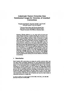
Fig. 3: 3D point cloud data from NTU’s School of Communications.

360 degree scan is performed. The environment is then represented by batches of horizontal planes at each elevation angle. Figure 3 shows a point cloud, again of NTU’s School of Communication. The scan resolution in this case was 720 points per 360o sweep, at 60 elevation angles between ±15o of the horizontal scanning plane. The scans took 15 seconds to record, at this resolution with this scanning system. III

Fig. 1: The panoramic vision and 3D laser range finder. stitched image to give a 360o field of view of the environment. To use information from both sensors, correspondents need to be found, so an approximate calibration between the two sensors is necessary.

3D P RINCIPAL C OMPONENT A NALYSIS (PCA)

PCA is a powerful tool which can determine dominant data directions within entire data sets, and use these to represent the data in a compressed form with little loss of information [9]. A brief overview of the algorithm is now presented, along with the problems it yields when naively applied to 3D laser range data. Assuming a 3D set of data X = {xi , yi , zi } with i = 1, 2, ..., n, the means xm , ym and zm of the data set of each coordinate value, are given by: n

II-A

Ladybug 2 Panoramic Camera

The Ladybug-2, panoramic camera is a spherical digital video camera system. It consists of 5 cameras at the side of the cylinder covering 360 degrees, and another camera on the top. 6 images are produced simultaneously. An image stitching algorithm has been developed to merge the 6 images together and generate a stitched image with a 360o panoramic view. The stitching process determined the intrinsic and extrinsic parameters of the camera system, so that the overlapping regions of each individual camera could be determined and aligned to stitch the six images together. Figure 2 shows an image of NTU’s School of Communication after the stitching process.

Fig. 2: A “stitched”, panoramic image of NTU’s School of Communications. II-B

3D Laser Range Finder

An illustration of a scan using the 3D LADAR is shown in Figure 3. At each elevation angle, a full horizontal

xm =

n

n

1X 1X 1X xi , y m = yi , zm = zi n i=1 n i=1 n i=1

(1)

where n is the number of points per 3D scan. By subtracting the relevant mean from each data point the data variance terms can be calculated as: n 1 X 2 σxx = (xi − xm )2 , (2) n − 1 i=1 n

2 σxy

=

1 X (xi − xm )(yi − ym ), etc. n − 1 i=1

2 2 is the cross where σxx is the variance of x and σxy covariance between x and y variables. This yields a 3-by-3 square matrix with elements  2  2 2 σxx σxy σxz 2 2 2  σyy σyz C =  σyx (3) 2 2 2 σzx σzy σzz

Figure 4 shows the results of applying PCA to the real data set of figure 3. The axes shown in red, represent the ellipsoid of the covariance matrix from equation 3. The lengths of these correspond to the eigenvalues of the matrix, and their directions lie in the corresponding directions of their eigenvectors. The axes lengths in the figure are of comparable magnitudes, and hence do not detect any dominant data directions within the point cloud, indicating a “random”

Fig. 6: Range-colour calibration. Each 3D point has a range, bearing, elevation and red, green, blue intensity value.

Fig. 4: PCA covariance matrix principal directions superimposed on the point cloud data of figure 3.

nature to the data. If however, an appropriate portion of the point cloud is removed from the figure, this results in figure 5, where the eigenvalue axis lengths are 2.0, 7.01 and 17.01 respectively. One of the axis lengths is significantly smaller

Fig. 5: A subset of the point cloud of figure 3, with its covariance matrix principal directions superimposed. than the other two, which indicates 2 dominant directions in the point cloud data. This implies that the 3D point cloud subset can be approximately represented as a 2D plane, as is visually evident as most of the data comes from the flat ground. This indicates that some form of segmentation of the full, 3D, point cloud data sets is necessary before PCA can be successfully applied. Therefore, colour information from the Ladybug-2 panoramic camera is to be used to first segment the 3D laser range data into suitable regions in which PCA can be applied with greater success. This first requires an approximate calibration between the laser range points, and their corresponding colour intensity values in the camera image. IV

3D LADAR - C AMERA C ALIBRATION

The aim of the calibration of the panoramic camera system and laser range finder is to produce 3D colour

registered laser range data, as shown in figure 6. The laser range finder yields point cloud data of the form P (ρ, α, β) where ρ is the range to the point, α is its bearing angle with respect to a datum on the sensor and β is its elevation angle. The calibration method described in [8], in which known correspondents in the real world between their laser range points P (ρ, α, β) and image pixel coordinates I(xi , yi ) with red, green, blue intensity values [ri , gi , bi ]T is used. This results in a transformation linking each laser range point with an image point (if it lies within the field of view of the panoramic camera), so that each laser range point can be augmented with colour information P (ρ, α, β, r, g, b), giving a coloured point cloud (the output in figure 6). By fusing the colour values of each pixel with the 3D point cloud, coloured 3D scans are obtained as shown in Figures 7 and 8. Since the calibration is not perfect, some

Fig. 7: Coloured 3D point cloud from NTU’s School of Communications.

Fig. 8: Coloured 3D point cloud within an indoor laboratory. points are indexed with the incorrect colour, this is due to errors in the transformation matrix. However, in terms of overall performance, the fusion gives a better visualization of the environment. Trees, walls, posters, objects and buildings possess textures and colours as their appearance in the real

world. The main point however is that, due to the colour information which is an addition attribute of the objects, feature identification can be easily achieved. V

I MAGE F ILTERING AND S EGMENTATION

As shown in section III, segmentation is of paramount importance before PCA can be successfully applied to range data. Accurate segmentation relies on smoothing sections of the image, whilst maintaining the localisation of the edges between these sections. Then, smoothed regions with approximately constant colour (HSV) values1 will be extracted to form segments. Numerous filtering methods exists which simultaneously attempt to preserve image edges. Anisotropic diffusion is an image smoothing method which prevents smoothing across edges by performing averaging in the orthogonal direction to the gradient of the luminance, which has also been directly applied to laser range data [1]. Its convergence properties are not however guaranteed under all image possibilities [12]. Bilateral filtering [10] is a non iterative scheme for edge preserving smoothing which combines colour space and spatial domain filtering. The Bilateral filter has been shown to produce excellent smoothing, but can degrade the localisation of the edges between different colour regions. The Mean shift algorithm [11] and [12], which is a non-parametric estimator of the density gradient in the spatial-colour range domain, is a useful tool for edge preserving, filtering and segmentation. The Mean shift algorithm is a clustering technique which does not require prior knowledge of the number of clusters and is therefore applied in this work. V-A

2) Initialize a new variable yk = xj , for each image pixel xj , where xj is a vector containing the spatial and range (colour) information P of pixel j. 3) Compute yk+1 = n1k xi ∈S1 (yk ) xi , where S1 (yk ) is a window with a predefined radius, centered on yk , and there are nk points are in the window. 4) Increment k, and repeat step 4 until convergence by checking k yk+1 − yk k< exp−3m where m is the greater value between hs and hr (defined below). r 5) Assign zi = (xsi , yconv ). This implies that image pixel at xj has the range (colour) components of the point r of convergence yconv . In this work, the spatial and range (colour intensity as an integer between 0 to 255) thresholds hs and hr were set to 8 and 7 respectively, and M (the minimum cluster size) was set to 100 pixels. These settings produced good results with moderate computational time. In order to examine how lighting affects the filtering process, indoor and outdoor environments were examined separately. The first batch of results are from the outdoor scene. The system was setup in front of the NTU communication school. It was recorded at noon and under a clear sky (figure 10). The other scene was inside the NTU Autonomous Robotics Research Laboratory (figure 11). The room was subjected to artificial lighting. Careful

Image Filtering: The Mean Shift Algorithm

The Mean Shift algorithm [11] and [12] makes use of a Kernel density estimation technique known as the Parzen window technique, which is the most popular density estimation method, to determine the convergent centroid of the window. The idea is to find the local maxima of a probability density on both the colour and spatial information within the image. Figure 9 illustrates the procedure of the algorithm, in which the points shown represent the spatial distribution of points within an image. Since an image is a combination

Fig. 10: Original (upper) and mean shift filtered (lower) images of NTU’s School of Communications.

Fig. 9: The Mean Shift algorithm – principle of operation. of spatial and colour spaces, the Mean Shift algorithm smoothes, but at the same time preserves the edges. To apply the Mean Shift algorithm to an image, for each j = 1...n, where n is the number of the image pixels we: 1) Initialize k = 1 1 Note

that Hue, Saturation, Value (HSV) colour coding is used, as it is less sensitive to ambient lighting than Red, Green, Blue (RGB) coding.

Fig. 11: Original (upper) and mean shift filtered (lower) images of NTU’s Autonomous Robotics Research Lab. examination of both scenes shows that successful smoothing and image edge preservation is possible in both outdoor and indoor environments.

V-B

Segmentation

After image filtering, a clustering process takes place. The aim is to segment the image into small regions according to the closeness of spatial and colour range information after the filtering process. This is so that the corresponding laser point cloud data can be extracted for PCA to be applied. An algorithm is applied to find the connectivity between neighbouring pixels. Two pixels are considered as connecting to each other if their difference in spatial and range (colour) value is less than the given threshold (hs and hr ). A label index is assigned to the cluster to differentiate one from another. Then, based on this cluster index, the range data is segmented and PCA is applied to determine if the data forms a line or a plane. The process can be illustrated as the flow chart shown in Figure 12. First, a

Fig. 14: The final connectivity matrix and labeled clusters.

by another parameter M . Clusters whose number of pixels fall below the value of M are eliminated. In this case, the value of M is set to 100 pixels. Label value 0 is assigned to pixels which do not belong to any cluster. Figure 15

Fig. 12: Flow diagram: Visually aided range segmentation. connectivity matrix is initialized as shown in Figure 13. It is a binary matrix. If m and n are the width and height of the given image, the connectivity matrix is initialized with the size of (2m+1)×(2n+1). Binary 1 is assigned to locations {2i, 2j} for all i = 1, 2, ..., m and j = 1, 2, ..., n. Binary 0 is assigned to the remaining cells of the matrix. This ensures that every “1” is surrounded by “O”s. The left, right, top and bottom cells of each binary 1 will contain the information between the image pixel with its left, right, top and bottom neighbours respectively. Binary 1 is assigned to the cell if the difference for both spatial and range value between the two cells is below the given threshold (hs = 8 and hr = 7), and binary 0 otherwise. Figure 14 is an example of the final output of the connectivity matrix. After all binary 1s and 0s are filled in the matrix, based on the comparison made between each pair of adjacent pixel values, the connectivity test takes place to group all the pixels which connect to each other. In Figure 14, three clusters are formed. In order to facilitate range data segmentation later, the colour value of each pixel is replaced by the cluster label. In the Mean Shift algorithm, the clustering is constrained

Fig. 13: Initialization of the connectivity matrix.

Fig. 15: Mean Shift filtering and segmentation. shows the result of Mean Shift filtering and segmentation. It highlights one section of the image undergoing filtering and segmentation. Different clusters are visualized by using different colours as shown in Figure 16.

Fig. 16: Segmented image of the School of Communications. It can be observed that some regions (shown in the original image colour) didn’t belong to any clusters. This is because these regions were assigned a number of pixels less than the value of M . In Figure 15, it is clear that there are two clusters and a stripe (horizontally in the middle of the highlighted boxes in Figure 15) which doesn’t belong to any of the two clusters. Figure 17 shows the cluster map corresponding to the cut region of the image. Three values appear in the map. Numerical figures 38 and 40 represent two clusters respectively, where 0 represents those pixels not belonging to any clusters in the map. cluster labels from the image space are then attached to each range data point to assign that particular range point to the cluster. The central images in figures 18 and 19 show the coloured point cloud data from figures 7 and 8 respectively, and their respective colour segmentation. The different colours represent different clusters or objects in the environment.

Fig. 17: Segmentation labeling and clustering. VI PCA WITH S EGMENTED R ANGE DATA After range segmentation, PCA is applied to the segmented data as represented in Figure 12. Figures 18 and 19 show the results of applying PCA to the segmented range data from the outdoor and indoor environments respectively. The range data is segmented according to the number of the clusters in the image. The cluster index number tag is attached to each range data point to identify which cluster that particular range data belongs to. Moreover, the range data can now be sorted based on the cluster index number. For each cluster, the range data undergoes PCA to determine whether the data belongs to a plane, a line or is randomly distributed over the, now reduced, segmented space. For each point cloud cluster, their mean and covariance are calculated. Then, the eigenvalues of the covariance matrix (equation 3) are obtained. In figures 18 and 19, the bold red lines in each segmented range image represent the axes of the ellipsoid of the covariance matrix. In this particular case, a ratio test is carried out for each set of eigenvalues. For i = 1, 2, 3, assuming λi , to be the eigenvalues of the data set, their ratios are defined as λi (4) Ti = λ1 + λ2 + λ3 These ratios determine the categories of the data. If one, two or none of the Ti is/are smaller than the given threshold T , it indicates that the data set is estimated to be approximately on a 2D plane, co-linear or randomly scattered (meaning no extracted features) over the given space respectively. For the outdoor scene, 12 sets of segmented range data corresponding to 12 clusters of the image are found (figure 18), and 9 segments are found in the indoor scene (figure 19). PCA was then applied to each set of segmented point cloud data, resulting in the successful detection of planer sections within the 3D environments. The threshold T was set to 1%, for the accepted detection of lines or planes. For example, for cluster 12 in figure 18, the eigenvalues λ1 , λ2 and λ3 of the covariance matrix are 8.205, 80.40 and 176.198 respectively, giving ratios (equation 4) T1 = 3.09%, T2 = 30.29% and T3 = 68.72%, all of which are greater than T = 1%. Therefore, this data segment is assumed random, although 2 of the directions dominate. This makes sense, since that section of the image shows a section of a building wall (planar) which is corrupted with trees and their shadows on the floor. This is clearer in figure 20. 2 The index is shown on the corner of each segmented point cloud set in figures 18 and 19.

Fig. 18: PCA applied to the segmented outdoor scene.

In cluster 10 the eigenvalue ratios are 0.09%, 24.01% and 75.9% respectively, and the data is assumed to be approximately co-planar. The normal of the plane can be determined from the eigenvector corresponding to the smallest eigenvalue: u = −0.0146i−0.0043j+0.9999k which makes sense (figure 21) since that portion of scan corresponds to the floor and has a normal in the z-axis direction. In cluster 5 of figure 19 the eigenvalue ratios are 0.21%, 47.47% and 52.32%. T1 is once again smaller than the threshold, and the eigenvector corresponding to λ1 is u = 0.1552i + 0.9879j + 0.0024k. This plane is perpendicular to the y-axis and is a section of the vertical wall (figure 22). VII

C ONCLUSIONS

PCA is a simple, yet powerful technique capable of representing large 3D data sets in terms of their dominant directions. It was demonstrated that if the data can first be segmented, then PCA could yield useful and efficient features from the segmented subset of the data. To carry out the segmentation process of 3D point cloud data, an integrated 3D laser range finder and panoramic camera system was built and described. After an approximate calibration, the system was able to provide 3D point cloud data with augmented HSV colour information. The Mean Shift image smoothing algorithm allowed the image to be segmented into clusters, which were then used to segment the corresponding 3D point cloud data into smaller groups. Finally, PCA was applied to each of these groups to categorize the data as planar, linear or random in form. The results showed a high performance in terms of plane

Fig. 21: Segment 10 from figure 18 - a horizontal plane.

Fig. 19: PCA applied to the segmented indoor scene. Fig. 22: Segment 5 from figure 19 - a vertical plane.

could then be trimmed in a methodical manner, dependent on the relationship between 3D range points and image points, to remove possible out-lier data, which could then be used to automatically adjust the calibration parameters. This is a focus of our ongoing research. R EFERENCES

Fig. 20: Segment 1 from fig. 18 and its dominant directions.

extraction, in both indoor and outdoor environments, and yielded their planar surface normals. It should be noted however that misclassification between laser range and image data can occur due to several factors: 1) Calibration errors can cause colour values to be assigned to the wrong range data points; 2) Different objects having the same colour can be clustered into the same group; 3) Single objects having several colours can be split into groups of clusters; 4) Different lighting conditions can cause different segmentation results. Since only dominant directions are determined within subsets of 3D point clouds, the presented feature extraction method is robust to small amounts of the above errors. As an extension to this work, an error feedback system could be possible to minimize the calibration error. A cluster from an image is linked to a certain subset of the range data, through the calibration. If the corresponding range point subset then fails to yield PCA based dominant directions, the calibration could be erroneous. The range data subset

[1] M. Adams, F. Tang and W. S. Wijesoma. Convergent Smoothing and Segmentation of Noisy Range Data in Multiscale Space. IEEE Trans. on Robotics, pp. 746-753, June 2008. [2] D.F. Huber, and M. Hebert, A New Approach to 3-D Terrain Mapping, International Conference on Intelligent Robots and Systems (IROS), Kyongju, Korea, October 1999. [3] D. Viejo and M. Cazorla. Plane Extraction and Error Modeling of 3D data. Intl Symposium on Robotics and Automation, August 2006. [4] R. Triebel, W. Burgard and F. Dellaert, Using Hierarchical EM to Extract Planes from 3D Range Scans. In Proc. of the IEEE International Conference on Robotics and Automation (ICRA), 2005 [5] J. Horn, G. Schmidt, Continuous localization of a mobile robot based on 3D-laser-range-data, predicted sensor images, and dead-reckoning, Robotics and Autonomous Systems, 1995, v. 14, pp. 99-118 [6] J. Weingarten, G. Gruener, R. Siegwart, A Fast and Robust 3D Feature Extraction Algorithm for Structured Environment Reconstruction, Proceedings of ICAR, 2003, Coimbra. [7] P. Chakravarty, R. Jarvis, Panoramic Vision and Laser Range Finder Fusion for Multiple Person Tracking, in Proc. IEEE Int. Conf. Intelligent Robots and Systems, pp.2949-2954, 2006. [8] Y. Tsai, A versatile camera Calibration Technique for High-Accuracy 3D Machine Vision Metrology Using Off-the-Shelf TV Cameras and Lenses, IEEE Journal of Robotics and Automation, pp. 323-344, 1987. [9] Linsey Smith. A tutorial on Principal Component Analysis, 2002 [10] C. Tomasi and R. Manduchi, ”Bilateral Filtering for Gray and Color Images”, proc. of Intl Conf. Computer Vision, IEEE (1998) 839-846. [11] Y. Cheng. Mean shift, mode seeking, and clustering. IEEE Trans. Pattern Anal. Machine Intell., vol. 17, 790-799, 1995. [12] D. Comaniciu, P. Meer, Mean Shift Analysis and Applications, IEEE Int. Conf. Computer Vision, Kerkyra, Greece, 1197-1203, 1999. [13] A. Saxena, M. Sun, A. Ng, Make3D: Learning 3D Scene Structure from a Single Still Image, IEEE Trans. PAMI. 2008.