VLSI cell placement techniques - BS Computer Engineering

VLSI Cell Placement K. SHAHOOKAR Department University

AND P. MAZUMDER

of Electrical of Michigan,

Techniques

Engineering Ann

Arbor,

and

Computer

Michigan

Sc~ence,

48109

VLSI cell placement problem is known to be NP complete. A wide repertoire of heuristic algorithms exists in the literature for efficiently arranging the logic cells on a VLSI chip. The objective of this paper is to present a comprehensive survey of the various cell placement techniques, with emphasis on standard ce11and macro placement. Five major algorithms for placement are discussed: simulated annealing, force-directed placement, rein-cut placement, placement by numerical optimization, and evolution-based placement. The first two classes of algorithms owe their origin to physical laws, the third and fourth are analytical techniques, and the fifth class of algorithms is derived from biological phenomena. In each category, the basic algorithm is explained with appropriate examples. Also discussed are the different implementations done by researchers. Categories and Subject Descriptors: B.7.2 [Integrated Aids—placement and routing

Circuits]:

Design

General Terms: Design, Performance Additional Key Words and Phrases: VLSI, placement, layout, physical design, floor planning, simulated annealing, integrated circuits, genetic algorithm, force-directed placement, rein-cut, gate array, standard cell

INTRODUCTION

Computer-aided design tools are now making it possible to automate the entire layout process that follows the circuit design phase in VLSI design. This has mainly been made possible by the use of gate array and standard cell design styles, coupled with efficient software packages for automatic placement and routing. Figure la shows a chip using the standard cell layout style, which inc]udes some macro blocks. Standard cells (Figure lb) are logic modules with a predesigned internal layout. They have a

fixed height but different widths, depending on the functionality of the modules. They are laid out in rows, with routing channels or spaces between rows reserved for laying out the interconnects between the chip components. Standard cells are usually designed so the power and ground interconnects run horizontally through the top and bottom of the cells. When the cells are placed adjacent to each other, these interconnects form a continuous track in each row. The logic inputs and outputs of the module are available at pins or terminals along the top or bottom edge (or both). They are

This research was partially supported by the NSF Research Initiation Awards under the grant number MIP-8808978, the University Research Initiative program of the U.S. Army under the grant number DAAL 03-87-K-OO07,and the Digital Equipment Corporation Faculty Development Award. K, Shahookar is supported by the Science and Technology Scholarship Program of the Government of Pakistan. Permission to copy without fee all or part of this material is granted provided that the copies are not made or distributed for direct commercial advantage, the ACM copyright notice and the title of the publication and its date appear, and notice is given that copying is by permission of the Association for Computing Machinery. To copy otherwise, or to republish, requires a fee and/or specific permission. @ 1991 ACM 0360-0300/91/0600-0143 $01.50

ACM Computing Surveys, Vol. 23, No. 2, June 1991

144

“

K. Shahoohar

and P. Mazumder

CONTENTS

[INTRODUCTION Classification of Placement Algorithms Wire length Estimates 1 SIMULATED ANNEALING 11 Algorithm 12 Operation of Simulated Annealing 13 TlmberWolf 32 1.4 Recent Improvements m Simulated Anneahng z FORCE.DIRECTED pLAfJEMENT 2 1 Force-DwectedPlacement Techniques 2.2 Algorithm 2,3 Example 24 Goto’sPlacement Algorithm 25 Analysls 3 PLACEMENT BY PARTITIONING 3 1 Breuer’s Algorithms 32 Dunlop’s Algorithm and Termmal Propagation 33 Quadrlsectlon 34 Other Techmques 35 Analysls 4, NUMERICAL OPTIMIZATION TECHNIQUES 41 Eigenvalue Method 42 Resu%lveNetwork Optlmlzatlon 43 PROUD: Placement by Block Gauss-Seldel Optlmlzatlon 44 ATLAS: Techmque for Layout Using Analytlc Shapes 45 Algorithm for Block Placement by Size Optlmlzatlon 46 Other Work in This Field 5 PLACEMENT BY THE GENETIC ALGORITHM 5.1 Geme: Genetic Placement Algorlthm 5.2 ESP: Evolution-Based Placement Algorlthm 53 GASP Genetic Algorlthm for Standard Cell Placement 6 CONCLUSION ACKNOWLEDGMENTS References

connected by running interconnects or wires through the routing channels. Connections from one row to another are done either through vertical wiring channels at the edges of the chip or by using feed-through cells, which are standard height cells with a few interconnects running through them vertically. Macro blocks are logic modules not in the standard cell format, usually larger than standard cells, and placed at any convenient location on the chip. Figure 2 shows a chip using the gate array design style. Here, the circuit consists only of primitive logic gates, such as NAND gates, not only predesigned but ACM Computing Surveys, Vol 23, No 2, June 1991

prefabricated as a rectangular array, with horizontal and vertical routing channels between gates reserved for interconnects. The design of a chip is then reduced to designing the layout for the interconnects according to the circuit diagram. Likewise, fabrication of a custom chip requires only the masking steps for interconnect layout. Figure 3 shows a third chip layout style, which uses only macro blocks. These blocks may be of irregular shapes and sizes and do not fit together in regular rows and columns. Once again, space is left around the modules for wiring. For a detailed description of the layout styles, see Muroga [1982] and Ueda et al. [1986]. The placement problem can be defined as follows. Given an electrical circuit consisting of modules with predefined input and output terminals and interconnected in a predefined way, construct a layout indicating the positions of the modules so the estimated wire length and layout area are minimized. The inputs to the problem are the module description, consisting of the shapes, sizes, and terminal locations, and the netlist, describing the interconnections between the termi nals of the modules. The output is a list of x- and y-coordinates for all modules. Figure 4 provides an example of placement, where the circuit schematic of Figure 4a is placed in the standard cell layout style in Figure 4b. Figure 4C illustrates the Checkerboard model of the placement in which all cells are assumed to be square and of equal size and all terminals are assumed to be at the center of the cells. Thus, the length of the interconnect from one cell to the next is one unit. The main objectives of a placement algorithm are to minimize the total chip area and the total estimated wire length for all the nets. We need to optimize chip area usage in order to fit more functionality into a given chip area. We need to minimize wire length in order to reduce the capacitive delays associated with longer nets and speed up the operation of the chip. These goals are closely related to each other for standard cell and gate array design styles, since the total chip

Iz E&l

lnlnEam

❑

on

❑ 0[1

❑

❑ ❑ ❑

❑ ❑ ❑ ❑ ❑

ACM Computing

Surveys, Vol, 23, No 2, June 1991

146

.

K. Shahookar

and P. Mazumder

EIUUEIEIEI

❑ ❑

ATE~aaDtlaaaDa

In PAD

HORIZONTAL

CHANNEL ~

❑ ❑ •1

❑ ull Elncl Elcln 0000 ❑ 00 1317CICICIEIDCI ❑ 00 ❑ un ❑ oon ❑ non ❑ un ❑ un ❑ 00 Elan ❑ un ❑ on ❑ clrl ❑ nnncloncln

clclcl Elncincl nncl clclnnn unnclclcl ❑ izlclntl nclnclclnclaclcl tlclclclnlzclclclclnnnn ❑ lclnnnclclnnclclclcincl ❑ lnnclciclncltlnnclclncl ❑ lnnnnclclclnclnnclclcl .tlnnnnnnclclnclnan

❑ lclnclnnnciclclnnnn ❑ nnnclcl13clnnnDlJnn ❑ clcinElnElclnElclrJnclcl ❑ lnnnclclnclclnncluclcl clnnclcllJnnclnclclucln ❑ nclnclclnclnElclclclclcl ❑ lnclclnclnclnnclclclclcl ❑ lclclclclclnclclnclnucicl ❑ lclclclclclncl

Elclcicl Elunn

❑

EIEIEI

cl •1

❑ •1 •1 ❑

on

vERTIciLCHANNEL Figure 2.

Gate array layout style

area is approximately equal to the area of the modules plus the area occupiedby the interconnect. Hence, minimizing the wire length is approximately equivalent to minimizing the chip area. Inthe macro design style, the irregularly sized macros donotalwaysfit together, and some space is wasted. This plays a major role in determining the total chip area, andwe have atrade-off between minimizing area andminimizingthe wire length. In some cases, secondary performance measures, such as the preferential minimization of wire length of a few critical nets, may alsobe needed, at the cost ofan increase in total wire length.

ACM Computmg

Surveys, Vol. 23, No. 2, June 1991

Another criterion for an acceptable placement is that it should be physically possible; that is, (1) the modules should not overlap, (2) they should lie within the boundaries of the chip, (3) standard cells shouldbe confined to rows inpredetermined positions, and (4) gates in a gate array should be confined to grid points. It is common practiceto define a function, cost function or an objective which consists of the sum of the total estimated wire length andvariouspenalties for module overlap, total chip area, and so on. The goal of the placement algorithm is to determine a placement with the minimum possible cost.

VLSI

❑

Cell Placement

on

Techniques

n

147

nan

C—3 L___.d

●

WASI’EI) .$PACE

El

HOR mu-= CHANNEL

❑

[1

[n n

-1

❑ pnclncl

❑ •1 ❑ ❑ ❑ •1

!

VERTICAL CHANNEL Figure 3.

Macro block layout style

Some of the placement algorithms described in this paper are ‘suitable for standard cells and gate arrays, some are more suitable for macro blocks, and some m-e suitable for both. In this paper, the words module, cell, and element are used to describe either a standard cell or a gate (or a macro block, if the algorithm can also be used for macros). The words macro and block are used synonymously in place of macro block. Their usage also depends on the usage in the original papers. Similarly, net, wire, interconnect, and signal line are used synonymously. The terms configuration, placement, and solution (to the placement problem) are

used synonymously to represent an assignment of modules to ‘physical locations on the chip. The terms pin and terminal refer to terminals on the modules. The terminals of the chip are referred to as pads. Module placement is an NP-complete problem and, therefore, cannot be solved exactly in polynomial time [Donath 1980; Leighton 1983; Sahni 1980]. Trying to get an exact solution by evaluating every possible placement to determine the best one would take time proportional to the factorial of the number of modules. This method is, therefore, impossible to use for circuits with alny reasonable number

ACM Computing Surveys, Vol. 23, No 2, June 1991

148

K. Shahookar

●

and P. Mazumder

A B~

D
C~~ Xn,, y~,) and the center gravity where

of the

net

Sk

be

Gk ( ~h,

The squared wire length of the (Figure 24a) is defined as

If m, is the total number objective function is defined

net

of nets, as

~h),

Sk

the

m’.

E-wk

w=

=

,:1,:1 {(~t - %)2+ (Yz- z)’}.

In macro placement, block orientation is important besides block position because of two reasons. In order to fit the irregularly shaped blocks together while minimizing the wasted space, all possible

VLSI

Module

Cell Placement

.

Techniques

189

pln

/

/,

A —

Net center

of gravity

(a)

(X’p, y~)

& (Xp, ,----

yp)

-%;-----

:

I t u I !

‘---

‘.

‘.

‘.

.

-------------------:

I

I I

I

‘.

1

h

‘“J3 ‘.

(x,,

Y il

------

;-----------~----:’

------

(X12, ------.

Y17) ---+

\

h,

(X f,yj)

?

‘:----+-

1’

(b) Figure 24. Squared euclidean after rotation in Atlas.

wire

length

function,

orientations should be allowed. Besides, rotation and mirroring have a significant effect on the wire length. If the pins on one side (left, say) of a large block are connected to other blocks placed on the other side (right), then the nets are forced to go around the block. Flipping the block over reduces the wire length. Block through

Rotation. an angle

If a block is rotated 6’, the pin coordinates

‘w’ Wk = AG2 + BG2 + CC,2 + DG2;

( ~~, y:) relative given by

to the

(b) pin

block

position

center

are

x; = XPCOS6 –yPsin6, y~=yPcos

O+xPsin

O,

where x and yP are the original coordi nates re f“atlve to the block center (Figure 24b). Let the block axis be defined by the pair of coordinates ( X,l, y,l) and ( $,Z, Y,z) and the block

ACM Computing

center

Surveys, Vol

be denoted

23, No 2, June 1991

190 by

“

K. Shahookar

and P. Mazumder

(+, Y,). Let

AY,

=IY,l–

d, = al=—,

Let the block width be w, and the block height be h,, with 1, = w, – h,, and Ax,, A y,, and d, be as defined above. The constraint that prevents block overlap is given by

Y,217

~Xp

gl(i,~)

= r,+

r~ – d(i,

~) = 0;

d, ()+—.

Yp d,

Then, we get after rotation:

the

absolute

x jJL = XL + alAx,

pin

position

– azliy,,

r,, rJ are the block radii (half the block height), and d( i, j) is the distance between the axes of the blocks i and j. For the derivation, see Sha and Dutton [19851. Only two block orientations, vertical and horizontal, are allowed. To ensure this, the orientation constraint is used:

gz(i) The new parameters introduced in objective function are constants and yp. Since no new variables introduced, there is little increase computation time.

the XP are in

Mirroring. The mirroring operation is realized by introducing an extra vari able, u,, such that u, = 1 means normal orientation and u, = – 1 means mirrored orientation. The pin position is now given by x pL = x,

+

alAxZ

–

Uzcy2fiyL,

gs(i)

4.4.3

ACM Computing

Surveys, Vol. 23, No. 2, June 1991

. . ..m.

= Z,–

d, =0.

Let the desired chip aspect ratio be q, with the vertical and horizontal dimensions y~ and x~ = qyn, respectively. Then, the boundary constraints are

4.4.2

In addition to the above objective function, some constraints are imposed during the solution process in order to ensure a legal placement. These constraints are only summarized here. For a detailed discussion, see Sha and Dutton [1985].

i=l,2,

It is obvious that if the block is not vertical or horizontal, both Ax, and A y, will be nonzero, and the constraint will not be satisfied. The constraint for the desired block size is given by

forl=l,2;

Conditions

Ay, /lt=O

for

These pin coordinates are used along with the block coordinates in order to calculate the wire length more accurately. During optimization, u, is treated as a continuous variable that can vary within the bounds I UZ I = 1. A constraint (u, – l)(uZ + 1) = O is imposed during the optimization process. This constraint makes u converge to either + 1 or – 1. Constraint

= Ax,

g41z(i)

= r, – Xtz~O,

g42z(i)

= r, – YLz~O,

g43~(i)

= x,z + r, – .r~=o,

g..l(i)

= Y,, + T-c- ym~o,

Penalty

The penalty the following (1)

Select typically

i=l,2,

. . ..m.

Function

Method

function method procedure: an

co = 1;

increasing

consists

series

Ck+l = lock.

of

Ck,

VLSI

Cell Placement

Techniques

“

191

(a)

(c)

(b) Figure 25.

(a)

PFM optimization

process: Intermediate

Construct a new unconstrained objective function P( x, c~) such that P( x, y, Ch) = objective + Ck~

function constraints.

(3) Use an unconstrained optimization technique such as Newton’s method to minimize P( x, y, c~) for k = 0,1,2,. ... until the coordinates of the modules satisfy the constraints within the required accuracy. Thus, in PFM during the first iteration, the constraints are reemphasized

results

n D

as Cfi is increased.

and a solution is obtained. Fimre 25a shows the result of the first iteration, with c~ = 1. Then, in each iteration the weight of the constraints is increased and the objective function minimized. This causes the constraints to be satisfied more and more accurately, at the expense of an increase in the value of the objective function. An intermediate result is shown in Figure 25b. As c~ is increased, the modules attain the proper orientation and overlap is reduced. The process is terminated when the ccmstraints are satisfied within the desired accuracy. Figure 25c shows the final result, with all modules

ACM Computing Surveys, Vol. 23, No. 2, June 1991

192

●

K. Shahookar

and P. Mazumder

in either vertical or horizontal tion and no overlap.

4.4.4

Comparison

with Simulated

orienta-

Annealing

PFM uses numerical techniques, whereas simulated annealing uses a statistical approach. Although the techniques of nonlinear programming and simulated annealing are very different, some simi larities exist. The parameter c~ in PFM behaves like the reciprocal of temperature (1/ 7’) in simulated annealing. In simulated annealing, moves are randomly generated, whereas in PFM moves are deterministic and are in the direction that minimizes the penalty function P( x, y, c~). The important feature of PFM is that all blocks move simultaneously, not one at a time as in simulated annealing. PFM has been tested on two chips with 23 and 33 macro cells, and the results have been compared to those of TimberWolf and industrial placement. A 50% improvement over industrial placement and 23% improvement over TimberWolf were reported. The CPU time reported is of the order of 2 h on a VAX station II for a 33-block circuit. 4.5

Algorithm

for

Block Placement

by Size

Optimization One example of linearization is provided by Mogaki et al. [19871. They presented an algorithm for the placement of macro blocks to minimize chip area under constraints on block size, relative block position, and the width of the available interlock routing space. This algorithm iteratively determines the optimum block size and relative block placement in order to reduce the wasted space and minimize the total chip area. Channel widths are also considered during the optimization process. This is a quadratic integer programming problem, which has been reformulated as a linear programming problem and solved by the Simplex method. This algorithm is the extension of the work of Kozawa et al. [1984], and uses their Combined and Top Down

ACM Computing

Surveys, Vol. 23, No 2, June 1991

Placement (CTOP) algorithm for the actual block placement. This is coupled with block resizing by linear programming. This algorithm is suitable only where block sizes are not yet fixed and macro blocks can be generated with a range of possible aspect ratios. Hence, choosing the block aspect ratios to fit together nicely in the placement, then generating the macro blocks results in a compact layout. The first step is to generate an initial placement by the CTOP algorithm. This algorithm works by repeatedly combining two blocks to form a hyper-block until the entire chip consists of one hyper-block. At each step, blocks are paired so as to minimize the wasted space and maximize their connectivity to each other. Repeated combining of blocks generates a combine tree with the entire chip as the root node and the individual blocks as leaves. This tree is then traversed top down, such that for each hy per-block, a good placement is determined for its component blocks. This gives the relative placement of the blocks. The relative placement is converted to a Block Neighboring Graph (BNG), as shown in Figure 26. Each block is represented as a node in the BNG, and each segment of a routing channel between two blocks is represented by an edge connecting the nodes. Formally, BNG

= G(V,

E)

such that V=

{u} U{ L, R, B, T};

EC

VXVX{X,

Y}

X{6},

where u represents a block, L, R, B, T are the simulated blocks corresponding to left, right, top, and bottom edges of the chip, X or Y represent whether the channel is vertical or horizontal, and 8 > 0 represents the minimum channel width. The next step is the linear programming formulation for block size optimization. This consists of the objective function and the constraints.

VLSI

Cell Placement

Techniques

.

193

u F1 7

-k

Y.

El

En t–– x“

‘“

--+j~uvy xv

Example macro-block layout and its block neighboring graph. ❑ , Block; o, simulated block; + , vertical edge; ---> , horizontal edge.

Figure 26.

4.5.1

Objective

Function

The primary objective is to minimize the chip area. Wire length is considered indi rectly through its effect on the chip area. There is a user-specified limit on the chip

aspect ratio. Let the minimum mum desirable values of the ratio be ~. and r+: r–~

and maxichip aspect

Y — 0, the chip area function can be replaced by rx + y, which is a linear function, because r is a constant. Thus, in order to minimize chip area xy, the linear programming problem is formulated to minimize rx + y. The effect of this linearization is shown in Figure 27. The shaded region represents the allowed values of chip width and height. This region is bounded by the maximum and minimum chip area constraints and the maximum and minimum aspect ratio constraints. Within a small aspect ratio range, the linearized area is a good approximation to the actual area. ACM Computing Surveys, Vol. 23, No. 2, June 1991

objective

function,

Constraints

Block size constraint. Each block has a given range of candidate sizes where i = given by (wU(i), h“(i)), 1,2,. ... Nu. Nu is the number of posu. The object of sible sizes for block the linear programming approach is to choose the aspect ratio that results in the minimum wastage of chip area. Let AU(i) be the selection weight for the ith candidate block size such that

~ Au(i) 1=1

= 1,

Ox,~uu)=~, as shown in Figure 26. Similarly, if block u is below block U, we get the corresponding constraint Y“–

(Yu + Wu) =6.”

These constraints determine an size when the specified.

E.

make it possible to appropriate block channel widths are

Thus, the objective of the linear programming formulation is to determine XU, yU, WU, hU for all blocks u so that the linearized area r-x + y is minimized, subject to the above constraints. 4.5.3

Procedure

The algorithm follows:

can

be

summarized

as

(1) Determine

the relative block placement by the CTCDP algorithm [Kozawa et al. 1984].

(2) Determine ment by procedure:

the the

absolute following

block placerepetitive

(2.1)

Determine the channel global routing.

(2.2)

Optimize following rithm: (2.2.1)

(2.2.2)

(2.2.3)

Techniques

Solve the LP problem the Simplex method.

(2.2 .4) Select closest tion. (2.3)

*

the block to the LP

195 by size scdu-

(]0 to 2.1

The algorithm has been tested on two chips with up to 40 macro blocks. Experimental results indicate that 690 saving of area can result over manual designs and 5-10% over other algorithms. This saving is achieved, however, at the cost of 10-12 times the computation time compared to other algorithms. 4.6 Other \(Vork in This Field

for each edge (u, u, Y,8Uu]e

Cell Placement

width

by

block size using the optimization algo Generate the BNG the relative block tions.

from posi-

Eliminate redundant constraints and convert the rest into an LP condition matrix.

Blanks [1985a, 1985b] has exploited the mathematical properties of the quadratic (sum of squares) distance metric to develop an extremely fast wire length eval uation scheme. He uses the eigenvalue method to determine the lower bound on the wire I ength in order to evaluate his iterative improvement procedures. He has also given a theoretical model to explain the observed deviation from optimality. Markov et al. [1984] have used Bender’s [1962] procedure for optimization. Blanks [1984] and Jarmon [1987] have used the least-squares technique. Akers [1981] has used linear assignment. He has given two versions-constructive placement and iterative improvement. Further work on the eigenvalue method has been done by Hanan and Kurtzberg [1972bl. Hillner et al. [19861 has proposed a dynamic programming approach for gate array p Iacement (see also Karger and Malek [19841). Herrigel and Fichtner 11989] have used the Penalty Function Method for macro placement. Kappen and de Bent [1990] have presented an improvement over Tsay et al.’s algorithm discussed in Section 4.3. 5. PLACEMENT ALGORITHM

BY THE GENETIC

The genetic algorithm is a very powerful optimization algorithm, which works by emulating the natural process of evolution as a means of progressing toward ACM Computing

Surveys, Vol. 23, No. 2, June 1991

196

*

K. Shahookar

and P. Mazumder

the optimum. Historically, it preceded simulated annealing [Holland 1975], but it has only recently been widely applied for solving problems in diverse fields, including VLSI placement [Grefenstette 1985, 1987]. The algorithm starts with an initial set of random configurations, called the population. Each individual in the population is a string of symbols, usually a binary bit string representing a solution to the optimization problem. During each iteration, called a generation, the individuals in the current population are eualuated using some measure of fitness. Based on this fitness value, individuals are selected from the population two at a time as parents. The fitter individuals have a higher probability of being selected. A number of genetic operators is applied to the parents to generate new individuals, called offspring, by combining the features of both parents. The three genetic operators commonly used are crossover, mutation, and inversion, which are derived by analogy from the biological process of evolution. These operators are described in detail below. The offspring are next evaluated, and a new generation is formed by selecting some of the parents and offspring, once again on the basis of their fitness, so as to keep the population size constant. This section explains why genetic algorithms are so successful in complex optimization problems in terms of schemata and the effect of genetic operators on them. Informally, the symbols used in the solution strings are known as genes. They are the basic building blocks of a solution and represent the properties that make one solution different from the other. For example, in the cell placement problem, the ordered triples consisting of the cells and their assigned coordinates can be considered genes. A solution string, which is made up of genes, is A schema is a set called a chromosome. of genes that make up a partial solution. An example would be a subplacement, consisting of any number of such triples, with ‘don’t cares’ for the rest of the cells. A schema with m defining elements and

ACM Computing

Surveys, Vol. 23, No 2, June 1991

‘don’t cares’ in the rest of the n – m positions (such as an m-cell subplace ment in an n-cell placement problem) can be considered as an (n – m)dimensional hyperplane in the solution space. All points on that hyperplane (i. e., all configurations that contain the given subplacement) are instances of the schema. Note here that the subplace ment does not have to be physically contiguous, such as a rectangular patch of the chip area. For example, a good subplacement can consist of two densely connected cells in neighboring locations. Similarly, a good subplacement can also consist of a cell at the input end of the network and a cell at the output end that are currently placed at opposite ends of the chip. Both of these subplacements will contribute to the high performance of the individual that inherits them. Thus, a schema is a logical rather than physi cal grouping of cell-coordinate triples that have a particular relative placement. As mentioned above, the genetic operators create a new generation of configurations by combining the schemata (or subplacements) of parents selected from the current generation. Due to the stochastic selection process, the fitter parents, which are expected to contain some good subplacements, are likely to produce more offspring, and the bad parents, which contain some bad subplacements, are likely to produce less offspring. Thus, in the next generation, the number of good subplacements (or highfitness schemata) tends to increase, and the number of bad subplacements (lowfitness schemata) tends to decrease. Thus, the fitness of the entire population improves. This is the basic mechanism of optimization by the genetic algorithm. Each individual in the population is an instance of 2‘ schemata, where n is the length of each individual string. (This is equivalent to saying that an n-cell placement contains 2” subplacements of any size. ) Thus, there is a very large number of schemata represented in a relatively small population. By trying out one new offspring, we get a rough estimate of the fitness of all of its schemata or subplace -

VLSI

FB:!:~J

Cell Placement

1, 1, ,1 ,,

Chromosomal

Rep.

Techniques

“

197

Cug

Physical

Layout

Figure 28. Traditional method of crossover. A segment of cells is taken from each parent. The coordinate array is taken from the first parent. With this method, cells B and F are repeated, and cells H and I are left out.

ments. Thus, with each new configuration examined, the number of each of its 2 n schemata present in the population is adjusted according to its fitness. This effect is termed the intrinsic parallelism of the genetic algorithm. As more configurations are tried out, the relative proportions of the various schemata in the population reflect their fitness more and more accurately. When a fitter schema is introduced in the population through one offspring, it is inherited by others in the succeeding generation; therefore its proportion in the population increases. It starts driving out the less fit schemata, and the average fitness of the population keeps improving. The genetic operators and their significance can now be explained. Crossover. Crossover is the main genetic operator. It operates on two individuals at a time and generates an offspring by combining schemata from both parents. A simple way to achieve crossover would be to choose a random cut point and generate the offspring by combining the segment of one parent to the left of the cut point with the segment of the other parent to the right of the cut point. This method works well with the bit string representation. Figure 28 gives

an example of crossover. In some applications, where the symbols in the solution string cannot be repeated, this method is not applicable without modification. Placement is a typical problem domain where such conflicts can occur. For example, as shown in Figure 28, cells B and F are repeated, and cells H and I are left out. Thus, we need either a new crossover operator that works well for these problem domains or a method to resolve such conflicts without causing significant degradation in the efficiency of the search process. The performance of the genetic algorithm depends to a great extent on the performance of the crossover used. Various operator crossover operators that overcome these problems are described in the following sections. When the algorithm has been running for some time, the individuals in the population are expected to be moderately good. Thus, when the schemata from two such individuals come together, the re suiting offspring can be even better, in which case they are accepted into the population. Besides, the fitter parents have a hligher probability of generating offspring. This process allows the algorithm to examine more configurations in a region of greater average fitness so the

ACM Computmg

Surveys, Vol. 23, No. 2, June 1991

198

●

K. Shahookar

CELL

4 ABC

and P. Mazumder

DE

Pm

+ FGHIJ

ABCDE

x 020507590030507095 Y 00 00 05050505050 SERIAL NO O , 23456709

F

GHIJ

J1 CELL AFCDEBGI+I,J x 020507590030557095 Y 0 0 0 0 0 50 505050W 1 umhan.ti SERIAL NO0 1 2 3456789 J

Chromosomal

Rep. Figure 29.

optimum may be determined and, at the same time, examine a few configurations in other regions of the configuration space so other areas of high average performance may be discovered. The amount of crossover is controlled by the crossover rate, which is defined as the ratio of the number of offspring produced in each generation to the population size. The crossover rate determines the ratio of the number of searches in regions of high average fitness to the number of searches in other regions. A higher crossover rate allows exploration of more of the solution space and reduces the chances of settling for a false optimum; but if this rate is too high, it results in a wastage of computation time in exploring unpromising regions of the solution space. Mutation. Mutation is a background operator, which is not directly responsi ble for producing new offspring. It produces incremental random changes in the offspring generated by crossover. The mechanism most commonly used is pairwise interchange as shown in Figure 29. This is not a mechanism for randomly examining new configurations as in other iterative improvement algorithms. In genetic algorithms, mutation serves the crucial role of replacing the genes lost from the population during the selection process so that they can be tried in a new context or of providing the genes that were not present in the initial popula-

ACM Computmg

Surveys, Vol

23, No 2, June 1991

Physical

Layout

Mutation.

tion. In terms of the placement problem, a gene consisting of an ordered triple of a cell and its associated ideal coordinates may not be present in any of the individuals in the population. (That is, that particular cell may be associated with nonideal coordinates in all the individuals.) In that case, crossover alone will not help because it is only an inheritance mechanism for existing genes. The mutation operator generates new cell-coordinate triples. If the new triples perform well, the configurations containing them are retained, and these triples spread throughout the population. The mutation rate is defined as the percentage of the total number of genes in the population, which are mutated in each generation. Thus, for an n-cell placement problem, with a population size NP, the total number of genes is nNP, and nNP R ~ /2 pairwise interchanges are performed for a mutation rate R ~. The mutation rate controls the rate at which new genes are introduced into the population for trial. If it is too low, many genes that would have been useful are never tried out. If it is too high, there will be too much random perturbation, the offspring will start losing their resemblance to the parents, and the algorithm will lose the ability to learn from the history of the search. Inversion. The inversion operator takes a random segment in a solution string and inverts it end for end

VLSI

Cell Placement

n A B C%-

CELL

020507590030557095

‘i

0000050

SERIAL NO

0

1

FGt+l

c)

,

ABC

x

0205030

‘t

GFEDHIJ

IIIll 0

9075557095

000550005050S0

SERIAL NO,

J

Each mll c..rd!na!e wle unchanged >

/ .,,,

199

Em

Y35050EQ 23456789

u

“

ABCDE

H I J

x

Techniques

0126543789

Chromosomal Rep.

Figure 30.

(Figure 30). This operation is performed in such a way that it does not modify the solution represented by the string; instead, it only modifies the representation of the solution. Thus, the symbols composing the string must have an interpretation independent of their position. This can be achieved by associating a serial number with each symbol in the string and interpreting the string with respect to these serial numbers instead of the array index. When a symbol is moved in the array, its serial number is moved with it, so the interpretation of the symbol remains unchanged. In the cell placement problem, the x- and y-coordinates stored with each cell perform this function. Thus, no matter where the cellcoordinate triple is located in the population array, it will have the same interpretation in terms of the physical layout. The advantage of’ the inversion operator is the following. There are some groups of properties, or genes, that would be advantageous for the offpsring to inherit together from one parent. Such groups of genes, which interact to increase the fitness of the offspring that inherit them, are said to be coadapted. For example, if cells A and B are densely connected to each other and parent 1 has the genes (A, xl, Yl) and (B, X2, Y2), where (xl, yl) and (X2, Y2) are neighboring locations, it would be advantageous for the offspring to inherit both these genes from one parent so that after crossover cells A and B remain in

‘ E!i%d >ABCDE

FGHIJ

Physical

Layout

[nversion. neighboring locations. If two genes are close to each other in the solution string, they have a lesser probability of being split up when the crossover operator divides the string into two segments. Thus, by shuffling the cells around in the solution string, inversion allows triples of cells that are already well placed relative to each other to be located close to each other in the string. This increases the probability that when the crossover operator splits parent configurations into segments to pass to the offspring, the subplacements consisting of such groups will be passed intact from one parent (or another). This process allows for the formation and survival of highly optimized subplacements long before the optimization of any complete placement is finished. The inuersion rate is the probability of performing inversion on each individual during each generation. It controls the amount of group formation. Too much inversion will result in the perturbation of the groups already formed.

Selection. After generating offspring, we need a selection procedure in order to choose the next generation from the combined set of parenk and offspring. There is a lot of diversity in the selection functions used by various researchers. This section briefly lists some of them. The following sections give the specific functions used in particular algorithms. The three most com]monly used selection

ACM Computing Surveys, Vol. 23, No. 2, June 1991

200

“

K. Shahookar

and P. Mazumder

methods are competitive, random, and stochastic. In competitive selection, all the parents and offspring compete with each other, and the P fittest individuals are selected, where P is the population size. In random selection, as the name implies, P individuals are selected at random, with uniform probability. Sometimes this is advantageous because that way the population maintains its diversity much longer and the search does not converge to a local optimum. With purely competitive selection, the whole populato individuals tion can quickly converge that are only slightly different from each other, after which the algorithm will lose its ability to optimize further. (This condition is called premature convergence. Once this occurs, the population will take a very long time to recover its diversity through the slow process of mutation.) A variation of this method is the retention of the best configuration and selection of the rest of the population randomly, This ensures that the fitness will always increase monotonically and we will lose the best configuration never found, simply because it was not selected by the random process. Stochastic selection is similar to the m-ocess described above for the selection if parents for crossover. The probability of selection of each individual is proportional to its fitness. This method includes both competition and randomness. Comparison with Simulated Annealing. Both simulated annealing and the genetic algorithm are computation intensive. The genetic algorithm, however, has some built-in features, which, if exploited properly, can result in significant savings. One difference is that simulated annealing operates on only one configuration at a time, whereas the genetic algorithm maintains a large population of configurations that are optimized simultaneously. Thus, the genetic algorithm takes advantage of the experience gained in past exploration of the solution a more extensive space and can direct cost. search to areas of lower average

ACM Computing

Surveys, Vol. 23, No. 2, June 1991

Since simulated annealing operates on only one configuration at a time, it has little history to use to learn from past trials. Both simulated annealing and the genetic algorithm have mechanisms for avoiding entrapment at local optima. In simulated annealing, this is done by occasionally discarding a superior con@-uration and accepting an inferior one. The genetic algorithm also relies on inferior configurations as a means of avoiding false optima, but since it has a whole population of configurations, the genetic algorithm can keep and process inferior configurations without losing the best ones. Besides, in the genetic algorithm each new configuration is constructed from two previous configurations, which means that in a few iterations, all the configurations in the population have a chance of contributing their good features to form one superconfiguration. In simulated annealing, each new configuration is formed from only one old configuration, which means that the good features of more than one radically different configurations never mix. A configuration is either accepted or thrown away as a whole, depending on its total cost . On the negative side, the genetic algorithm requires more memory space compared to simulated annealing. For example, a 1000 cell placement problem would require up to 400Kb to store a population of 50 configurations. For moderate sized layout problems, this memory requirement may not pose a significant problem because commercial workstations have 4Mb or more of primary memory. For circuits of the order of 10,000 cells, the genetic algorithm is expected to have a small amount of extra paging overhead compared to simulated annealing, but it is still expected to speed up the optimization due to the efficiency of the search process. The genetic algorithm is a new and powerful technique. This method depends for its success on the proper choice of the various parameters and functions that control processes like mutation,

VLSI selection, and crossover. If the functions are selected properly, a good placement will be obtained. The major problem in devising a genetic algorithm for module placement is choosing the functions most suitable for this problem, A great deal of research is currently being conducted on it. In this section, three algorithms due to Cohoon and Paris [19861, Kling [19871, and Shahookar and hkzumder [1990] are discussed. More work has been done in this field by Chan and Mazumder [19891. 5.1 Genie: Genetic

Placement

Cell Placement

Techniques

-

201

chosen, and the process is repeated. Experimental observations of Cohoon and Paris show that the initial population constructed by clustering is fitter, but it rapidly converges to a local optimum. Hence, in the final algorithm, they have used a mixed population, a part of which is constructed by each method. (z)

The scoring funcScoring function. tion determines the fitness of a place-

—

Algorithm

The Genie algorithm was developed by Cohoon and Paris [1986]. The pseudocode is given below: PROCEDURE Genie: Initialize; NP F population size; No+- & pi; /* where P+ is the desired ratio of the number of offspring Construct_ population(NP); FOR i -1 TO NP score(population[i]); ENDFOR; FOR i + 1 TO Number_ of_ Generations FORj-l TONo (Z, y) e Choose _Parents; offspring[ j] - generate _Offspring( x, y); Score(offspring[ j]); ENDFOR; population e Select(population, offspring, NP); FORj-l TONP With probability PWNlutate(population[j] ); ENDFOR: ENDFOR; ‘ Return highest scoring configuration in population; END. The following of the functions [19861 and their (1)

is a description used in Cohoon

of some and Paris

results.

Initial population construction. Cohoon and Paris [1986] proposed two methods for generating the initial population. The first one is to construct the population randomly. The second is to use a greedy clustering technique to place the cells. A net is chosen at random, and the modules connected to it are placed in netlist order. Then, another net connected to the most recently placed module is

to the population

size “/

ment. The scoring function u used in Genie uses the conventional wire length function based on the bounding rectangle. [t does not account for cell overlap or row lengths, owing to the gate array layout style. It does, however, acccmnt for nonuniform This is done as channel usage. follows: Let L, be the perimeter

of net

and c be this number columns, respectively, r

ACM Computing

Surveys, Vol

i,

of rows

and

23, No. 2, June 1991

202

“

K. Shahookar

and P. Mazumder chosen randomly, there is little improvement after several generations and hence no convergence to a good placement. The stochastic functions (3) and (4) produced the best results.

h, be the number of nets intersecting the horizontal channel i, U, be the number of nets intersecting the vertical channel i, .s~ be the standard

deviation

of h,,

SUbe the standard

deviation

of v,,

~ and U be the respectively,

_ .

mean

h,–~–s~

{

if

0

of

h,

and

(4) U,

~+s~ ‘#f Y, ‘,!,

2400032COOIXI -

-200000

. ,

12QOQI12uow

-240000

-160000

“1

:

\_

SOCa

0

Optimization

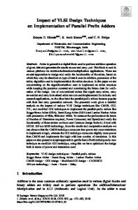
1000 2000 CPUSW(GASP) characteristics

an ideal location for them from force considerations and the other consisting of inter random/exhaustive pairwise change, with acceptance of the good moves and rejection of the bad moves, once again on the basis of force considerations. An overview of the various techniques used has been given, along with a sample algorithm and a network example to illustrate the operation of the algorithm. Goto’s GFDR algorithm has also been discussed. Placement is an optimization problem, and methods such as Simplex, Quadratic Programming, and the Penalty Function Method have traditionally been used for various linear and nonlinear optimization problems. Further, the placement problem can also be formulated in terms of the quadratic assignment problem, which can be solved by the eigenvalue method. Accordingly, several papers that use these techmques have been discussed under the category of numerical optimization techniques. The common feature of all these techniques is that they do not constrain the modules to grid points or rows, hence they are more applicable to macroblocks than to standard cells or gate arrays, although the solution generated by numerical techniques can be further processed to map the modules to the nearest grid points.

ACM Computing

Surveys, Vol. 23, No 2, June 1991

120000

80000 3000

of GASP compared to TimberWolf.

The final class of algorithms discussed here are genetic algorithms, which, although invented in the 1960s, were not used for placement until 1986. The genetic algorithm is an extremely efficient search and optimization technique for problems with a large and varied search space, as well as problems where more than one physical feature needs to be optimized simultaneously. The genetic algorithm processes a set of alternative placements together and creates a new placement for trial by combining subplacements from two parent placements. This causes the inheritance and accumulation of good subplacements from one generation to the next. It also causes the mixing of the good features of several different placements that are being optimized simultaneously for mutual benefit. Thus, the search through the solution space is inherently parallel. The placement problem is represented in the form of a genetic code, and the genetic operators operate on this code, not directly on the physical layout. This is a major deviation from the conventional placement algorithms that directly apply transformations to the physical layout. This intrinsic parallelism of the genetic algorithm can, however, be a potential problem, and unless a clever representation scheme is devised to represent the

VLSI Table 5.

Comparison of Placement

Algorithm

Implementation

algorithm

Huang et al. TimberWolf 3.2 Huang TimberWolf 3.2

Simulated Annealing

Dunlop and llernighan

Min-cut

Quadrisection TimberWolf 3.2 Quadrisection TimberWolf 3.2 Proud-2

Min-cut

Proud-4 TimberWolf TimberWolf Proud-2 Proud-4 TimberWolf TimberWolf Proud-2 Proud-4 ESP

Seidel

TimberWolf GASP TimberWolf GASP TimberWolf

Ver,f slow Very slow Slow medium Slow. medium Medium

Poor

Fast

Comparison of the Run Times of Placement

469 469 800 800

1.42 3 10.42

412

1

VAX

11/780

3.2 4.2

3,2 4.2

Evolution 3.2 Genetic 3.2 3.2

215

Speed

Near optimal Near optimal Medium. good Medium. . . good Good

No. of CPU Computer cells hours hardware

“

Algorithms

Algorithms

Performance

Reference

Wire lengths within k 4~o

[Huang

et al. 19861

10.7 VAX 11/780 Comparable manual

Gauss-

Techniques

Result quality

Simulated annealing Genetic algorithm Force directed Numerical optimization Min-cut Clustering and other constructive placement

Table 6.

Cell Placement

[Dunlop and Kernighan 19851

to layout

173 173 796 796 1438

0.01 VAX 8600 0.53 0.135 17.8 0.014 VAX 8650

Chip Chip Chip Chip Wire

area = area = area = area = length

1.11 1.0 0.91 1.0 = 0.93

1438 1438 1438 3816 3816 3816 3816 26277 26277 183

0.027 2 0.9 0.09 0.18 – 6.69 0.85 1,56 0.43

Wire Wire Wire Wire Wire Wire Wire Wire Wire Wire

length length length length length length length length length length

= = = = = = = = = =

183

2,7

469 469 800 800

11.0 11.3 12.5 13.7

Sun 3/75

Apollo-

DN4000

physical placement as a genetic code, the algorithm may prove ineffective. In this paper, three implementations of the genetic algorithm that overcome these different ways were problems in described. Table 5 is an approximate comparison of the performance of the algorithms dis cussed here. Table 6 gives the run time and performance of some of the algorithms. The wire length or chip area in the performance column has been nor-

= 1.0

Wire Wire Wire Wire

= = = =

1.0 1.02 1.0 0.87

19871

[Tsay et al. 19881

0.9 1.0 0.84 0.90 0.91 1.0 0.83 1.0 0.962 1.0 [Kling

Wire length length length length length

[Suaris and Kedem

19871

[Shahookar and Mazumder 19901

malized. This data can only give partial since different papers have comparisons, reported results on different circuits and have used different computer hardware. An attempt has been made to group the data according to the computer hardware used. Despite the bewildering variety of algorithms available, efficient module placement has so far remained an elusive goal. Most of the heuristics that have been tried take excessive amounts of CPU

ACM Computing

Surveys, Vol. 23, No 2, June 1991

216

0

K. Shahookar

and P. Mazumder

time and produce suboptimal results. Until recently excessive computation times had prohibited the processing of circuits with more than a few thousand modules. As fast simulated annealing and rein-cut algorithms discussed above are cast into fully developed place and route packages, however, this situation is expected to change. Preliminary re suits show that these algorithms have the capability to produce near-optimal placements in reasonable computation time. The following is a list of other surveys and tutorials on cell placement in order: Hanan and chronological Kurtzberg [1972 al, Press [19791, Soukup [19811, Chew [19841, Hu and Kuh [19851, Hildebrandt [1985], Goto and Matsuda [19861, Press and Karger [19861, Sangiovanni-Vincentelli [19871, Wong et al. [19881, and Press and Lorenzetti [19881. Robson [19841 and VLSI [1987, 19881 list exhaustive surveys on commercially available automatic layout software. These surveys indicate that forcedirected placement was the algorithm of choice in systems available in 1984 [Robson 1984]. In 1987 and 1988, we see an even mix of force-directed algorithms, rein-cut, and simulated annealing [VLSI 1987, 1988]. According to the 1988 survey, a few of these systems can be used to place and route sea-of-gates arrays with more than 100,000 gates, in triple metal, using up to 8090 of the available gates [VLSI 19881. Another trend immediately obvious from these surveys is that almost all the systems can be run on desktop workstations—Sun, Apollo, or MicroVAX. Thus automated layout systems are very widely available. They have made it possible to transfer the task of designing and laying out custom ICk from the IC manufacturer to the client.

ACKNOWLEDGMENTS This research was partially supported by the NSF Research Initiation Awards under the grant number MIP-8808978, the University Research Initiative program of the U.S. Army under the grant number DAAL 03-87-K-0007, and the Digital

ACM Computing

Surveys, Vol. 23, No. 2, June 1991

Equipment Corporation Faculty Development Award. K. Shahookar is supported by the Science and Technology Scholarship Program of the Government of Pakistan.

REFERENCES AARTS, E. H. L , DEBONT, F. M. J., AND HABERS, Statistical cooling: A general E. H. A. 1985. approach to combinatorial optimization prob lems. PhilLps J. Res. 40, 4, 193-226. AARTS, E. H. L., DEBONT, F. M. J., AND HABERS, implementations of E. H. A. 1986. Parallel Integration, the statistical cooling algorithm. VLSI

J. 4, 3 (Sept.)

209-238.

AKERS, S. B. 1981. On the use of the linear signment algorithm in module placement. Proceedings Conference.

of

the

18th

Des~gn

asIn

Automation

pp. 137-144.

ANTREICH, K. J., JOHANNES, F. M., AND KIRSCH, F H. 1982. A new approach for solving the placement problem using force models. In Proceedings of the IEEE International Symposmm on C%-cuits and Systems. pp. 481-486.

BANNERJEE, P., AND JONES, M. 1986. A parallel simulated annealing algorithm for standard cell placement on a hypercube computer. In Proceedings of the IEEE ence on Computer Design.

International p. 34.

Confer-

BENDERS, J. F. 1962. Partitioning procedures for Numer, solving mixed variable problems. Math.

4, 238-252.

BLANKS, J. P. 1984. Initial placement of gate arrays using least squares methods. In Proceedings of the 21st pp. 670-671.

Design

A utomatzon

Conference.

BLANKS, J, P. 1985a. Near-optimal placement using a quadratic objective function. In Pro. ceedmgs of the 22nd ference. pp. 609-615,

Deszgn

Automation

Con-

BLANKS, J. P. 19S5b. Use of a quadratic objective function for the placement problem in VLSI design. Ph.D. dissertation, Univ. of Texas at Austin. BREUER, M. A. 1977a.

Min-cut

sign Automation and ing 1, 4 (Oct.) 343-382.

BREUER,M. A. 1977b. ment Design

algorithms. Automation

Fault-

placement, Tolerant

A class of mm-cut

J. DeComput-

place-

In

Proceedings of the 14th Conference. pp. 284-290

CASSOTO, A.,

ROMEO, F., AND SANGIOVANNIVINCENTELLI, A. 1987. A parallel simulated annealing algorithm for the placement of stanDesign dard cells. IEEE Trans. Comput.-Aided CAD-6, 5 (May), 838.

CHAN, H. M., AND MAZUMDER, P. 1989. A genetic algorithm for macro cell placement. Tech. Rep. Computing Research Laboratory, Dept. of Electrical Engineering and Computer Science, University of Michigan, Ann Arbor, Mich.

VLSI CHANG, S. 1972. The generation of minimal trees with a steiner topology. J. ACM 19, 4 (Oct.), 699-711.

CHEN, N. P. 1983. New algorithms for steiner tree of the International on graphs. In Proceedings Symposium

on

Circuits

and

Systems.

pp.

1217-1219. CHENG, C. 1984. Placement algorithms and applications to VLSI design. Ph.D. dissertation Dept. of Electrical Engineering, Univ. of California, Berkeley. CHENG, C., AND KUH, E. 1984. Module placement IEEE based on resistive network optimization. Trans. Comput.-Aided Design CAD-3, 7 (July), 218-225. CHUNG, M. J., AND RAO, K. K. 1986. Parallel simulated annealing for partitioning and routof the IEEE International ing. In Proceedings Conference on Computer Design. pp. 238-242. CHYAN, D., AND 13REUER,M. A. 1983. A placement algorithm for array processors. In Proceedings of the 20th Design Automation Conference. pp. 182-188. COHOON, J. P., AND SAHNI, S. 1983. Heuristics for the board permutation problem. In Proceedings of the 20th

Design

Automation

Conference.

COHOON, J. P., AND PARIS, W. D. 1986. of the IEEE placement. In Proceedings tional Conference pp. 422-425.

on

placement capability of the In Proceedings Automation Conference. pp.

Design

A

DAVIS, L. 1985. Applying adaptive algorithms to of the Interepistatic domains. In Proceedings Joint

Conference

on Artificial

Intelli-

DONATH, W. E. 1980. Complexity theory and deof the 17th sign automation. In Proceedings Design Automation Conference. pp. 412-419. DUNLOP, A. E., AND KERNIGHAN, B. W. 1985. A procedure for placement of standard cell VLSI IEEE Trans. Comput. -Aided Design circuits. CAD-4, 1 (Jan.), 92-98. FIDUCCIA, C. M., AND MATTHEYSES, R. M. 1982. A linear-time heuristic for improving network of the 19th Design partitions. In Proceedings Automation Conference. pp. 175-181. FISK, C. J., CASKEY, D. L., m~ WEST, L. E. 1967. Accel: Automated circuit card etching layout. Proc. IEEE 55, 11 (Nov.) 1971-1982. FUKUNAGA, K., YAMADA, S., STONE, H., AND KASAI, T. 1983. Placement of circuit modules using a of the graph space approach. In Proceedings 20th

Design

Automation

Conference.

465-473.

GIDAS, B. 1985. Non-stationary Markov chains and convergence of the annealing algorithm. J. Stat.

21’7

●

algorithms for the o~uadratic assignment lem. J. SIAM 10, 2 (June), 305-313.

prob.

GOLDBERG, D. E., AND LINGLE, R. 1985. Alleles, loci and the traveling salesman problem. In Proceedings of the International Conference Genetic Algorithms and them Appl~catlons.

on

GOTO, S. 1981. An efficient algorithm for the two-dimensional placement problem in electriSyst., cal circuit layout. IEEE Trans. Circuits CAS-28 (Jan.), 12-18. GOTO, S., AND KUH, E. S. 1976. An approach to the two-dimensional placement problem in cirTrans. Circuits Syst. CAScuit layout. IEEE 25, 4, 208-214.

GOTO, S., CEDERBAUM, I., AND TING, B.S. 1977. Suboptimal solution of the backboard ordering IEEE Trans. with channel capacity constraint. Circuits

Syst.

(Nov.

1977),

645-652.

GOTO, S., AND MATSUDA, T. 1986. Partitioning, Design assignment and placement. In Layout And Verification, ‘T. Ohtsuki, Ed. Elsevier North-Holland, New York, Chap. 2, pp. 55-97. GREENE, J. W., AND SUPOWIT, K. J. 1984. Simulated annealing without rejected moves. In Proceedings of the IEEE ence on Computer Design.

International

Confer-

pp. 658-663. GREFENSTETTE, J. J., Ed. 1985. In Proceedings an International Conference on rithms and their Applications.

of

AlgoPittsburgh,

Genetic

GREFENSTETTE, J. J., Ed. 1987. the 2nd gorithms

International and their

In Proceedings

Conference Applications.

of Al-

on Genetic

Cambridge,

Mass.

406-413.

national gence.

Techniques

Penn.

CORRIGAN, L. I. 1979. based on partitioning. 16th

Computer-Aided

Genetic InternaDesign.

Cell Placement

Phys.

39, 73-131.

GILMORE, P. C. 1962.

Optimum

and suboptimum

GROVER, L. K. 1987. Standard cell placement usof the ing simulated sinte ring, In Proceedings 24th Design Automation Conference. pp. 56-59. HAJEK, B. 1988. Cooling schedules for optimal Oper. Res. 13, 2 (May), 311-329. annealing. HALL, K. M. 1970. An placement algorithm. (Nov.), 219-229.

r-dimensional Manage.

quadratic Sci.

17,

3

HANAN, M., AND KURTZ~ERG, J. M. 1972a. Placeof Digment techniques. In Design Automation ital Systems, 1, M A. Breuer, Ed. Prentice Hall, Englewood Cliffs, N. J., Chap. 5, pp. 213-282. HANAN, M., AND KURTZBERG, J. M. 1972b. A review of placement and quadratic assignment problems. SIAM Reu. 14, 2 (Apr.), 324-342. HANAN, M., AND WOLFF, P. K., AND AGULE, B. J. 1976a. Some experimental results on placeof the 13th ment techniques. In Proceedings Design Automation Conference. pp. 214-224. HANAN, M., AND WOLFF, P. K., AND AGULE, B. J. J. 1976b. A study of placement techniques. Design puting

Automation 1, 1 (Oct.),

and

Fault-Tolerant

Com-

28-61.

HANAN, M., WOLFF, P. IK., AND AGULE, B. J. 1978. Some experimental results on placement

ACM Computing

Surveys, Vol. 23, No. 2, June 1991

218

K. Shahookar

“

and P. Mazumder

techniques.

J. Deszgn Automation and Computing 2 (May), 145-168.

Tolerant

KERNIGHAN,B. W., AND LIN, S. 1970.

Fault-

HERRIGEL, A., AND FICHTNER, W. 1989. An analytic optimization technique for placement of of the 26th Design macrocells. In Proceedings Automation Conference. pp. 376-381. HILDEBRANDT, T. 1985. ACM bibliography. (Dec.), 12-21.

An annotated SIGDA

placement

Newsletter

15,

4

HILLNER, H., WEIS, B. X., AND MLYNSKI, D. A. 1986. The discrete placement problem: A dynamic programming approach. In Proceedings of the Internat~onal

Symposuim

HOLLAND, J. H. 1975. Artificial

Systems.

Press, Ann Arbor, Hu,

on Circuits

and

m Natural

and

pp. 315-318.

Systems.

Adaptation

University Mich.

of

T. C., AND KUH, E. S. 1985. Layout. IEEE Press, New York.

Michigan

VLSI

Cwcuit

HUANG, M. D., ROMEO, F., AND SANGIOVANNIVINCENTELLI, A. 1986. An efficient general cooling schedule for simulated annealing. In Proceedings of the IEEE ence on Computer-Aided

International ConferDesign. pp. 381–384.

“On Steiner Minimal HWANG, F. K 1976. SIAM J. with Rectilinear Distance,” Math. Vol. 30, PP.104-114, 1976

Trees Appl.

for HWANG, F. K. 1979. An O(n log n) algorithm IEEE suboptimal rectilinear steiner trees. Trans.

Cwcuits

Syst.

CAS-26,

1, 75-77.

JARMON, D. 1987. An automatic placer for arbitrary sized rectangular blocks based on a of the IEEE cellular model. In Proceedings International plicat~ons.

Conference

on Computers

and Ap-

pp. 842-845.

JOHANNES, F. M., JUST, K. M., AND ANTREICH, K. J. 1983. On the force placement of logic arrays. of the 6th European Conference In Proceedings on Cmcuit Theory and Design. pp. 203-206. JOHNSON, D. B., AND MIZOGUCHI, T. 1978. Selecting the kth element in X + Y and Xl + X2 J. Comput. 7, 2 (May), + . . . + Xm. SIAM 141-143

KAMBE, T., CHIBA, T., KIMURA, S., INUFUSHI, T , OKUDA, N., AND NISHIOKA, I. 1982. A placement algorithm for polycell LSI and its evaluaof the 19th De.wgn Aution. In Proceedings tomation Conference. PP 655-662 KANG, S. 1983. placement. Automation

Linear ordering and application to of the 20th Deszgn In Proceedings Conference. pp. 457-464.

KAPPEN, H. J., AND DE BONT, F. M. J. 1990. An efficient placement method for large standardof cell and sea-of-gates designs. In Proceedings the IEEE Conference.

European

Design

Automation

pp. 312-316.

KARGER, P. G., AND MALEK, M. 1984. Formulation of component placement as a constrained of the optimization problem. In Proceedings International Conference on Computer Design. pp. 814-819.

ACM Computing

Surveys, Vol. 23, No 2, June 1991

heuristic

procedure

Bell

Tech.

Syst.

for

partitioning

An efficient graphs.

J. 49, 2, 291-308.

KIRKPATRICK, S., GELATT, C D , AND VECCHI, M P. 1983. Optimization by simulated annealing. Sczence 220.4598 (May), 671-680. KLING, R. M, 1987. Placement by simulated evolution. Master’s thesis, Coordinated Science Lab, College of Engr., Univ. of Illinois at Urbana-Champaign. KLING, R., AND BANNERJEE, P. 1987. ESP: A new standard cell placement package using simuof the 24th Delated evolution. In Proceedings sign Automation Conference. pp. 60-66. KOZAWA, T., MIURA, T., AND TERAI, H. 1984. Combine and top down block placement algorithm for hierarchical logic VLSI layout. In Proceedings of the 21st pp. 535-542.

Design

Automation

Conference.

KOZAWA, T , TERAI, H., ISHII, T., HAYASE, M., MIURA, C., OGAWA, Y , KISHIDA, K., YAMADA, N., AND OHNO, Y. 1983. Automatic placement algorithms for high packing density VLSI. In Proceedings Conference.

of

the

20th

Design

Automation

pp. 175-181

KRUSKAL, J. 1956. On the shortest spanning subtree of a graph and the traveling salesman of the American Mathproblem. In proceedings ematical Soczety, Vol. 7, No. 1, pp. 48-50. VAN LAARHOVEN, P. J. M., AND AARTS, E. H. L. Simulated Annealing: Theory and Ap1987. plications. D. Riedel, Dordrecht-Holland. LAM, J., AND DELOSME, J. 1986. Logic minimization using simulated annealing. In Proceedings of the IEEE International Conference Computer-Aided Design. p. 378.

on

LAM, J., AND DELOSME, J. 1988. Performance of a of the new annealing schedule. In Proceedings 25th Design Automation Conference. pp. 306-311. LAUTHER, U, 1979. A rein-cut placement algorithm for general cell assemblies based on a of the graph representation. In Proceedings 16th Des~gn Automation Conference. pp. 1-10. Complexity LEIGHTON, F. T. 1983. MIT Press, Cambridge, Mass.

Issues

m VLSI.

LUNDY, M., AND MEES, A. 1984 Convergence of of the the annealing algorithm. In proceedings Szmulated

Annealing

Workshop.

MAGNUSON, W. G. 1977. A comparison IEEE structive placement algorithms. 6 Conf,

of conRegion

Rec. 28-32.

MALLELA, S., AND GROVER, L. K. 1988. Clustering based simulated annealing for standard cell of the 25th Design placement. In Proceedings Automation Conference. pp. 312-317. MARKOV, L. A., Fox, J. R., AND BLANK, J. H. 1984. Optimization technique for two-dimensional of the 21st Design placement. In Proceedings Automation Conference. pp. 652-654.

VLSI MITRA, D., RONIEO, F., AND SANGIOVANN1-VINCENTELLI, A. 1985. Convergence and finite-time behavior of simulated annealing. In Proceedings of Control.

the 24th Conference pp. 761-767.

on

Deciston

and

MOGAKI, M., MWRA, C., AND TERAI, H. 1987. Algorithm for block placement with size optimization technique by the linear programming IEEE International approach. In Proceedings Conference on Computer-Aided Design. pp. 80-83. MUROGA, S. 1982. ley, New York,

VLSI

System

John Wi-

Design.

Chap. 9, pp. 365-395.

NAHAR, S., SAHNI, S., AND SHRAGOWITZ, E. 1985, Experiments with simulated annealing. In Proceedings Conference.

of

the

22th

Destgn

pp. 748-752.

Conference Applications.

on

pp.

224-230. OmEN, R., ANDVAN GINNEKIN,L. 1984. Floorplan design using simulatecl annealing. In Proceedings of the IEEE International Conference Computer-Aided Design. pp. 96-98,

on

F’ALCZEWSKI, 1984. Performance of algorithms for of the 21st initial placement. In Proceedings Design Automation Conference, pp. 399-404. PERSKY, G., DEUTSCH, D. N., AND SCHWEIKERT, D. J., 1976. LTX: A system for the directed automatic design of LSI circuits. In Proceedings of the 13th

Design

Automation

Conference.

pp. 399-407. PREAS, B. T. 1979. Placement and routing algorithms for hierarchical integrated circuit layout Ph.D. dissertation, Dept. of Electrical Engr., Stanford Univ. Also Tech. Rep. 180, Computer Systems Lab, Stanford Univ. PREAS, B. T., AND KARGER, P. G. 1986. Automatic placement: A review of current techniques. In Proceedings Conference.

of

the

23rd

Destgn

Automation

pp. 622-629.

PREAS, B., AND LORENZETTI, M. 1988. Placement, assignment and floorplanning. In 20Physical Design Automation of VLSI Systems. The Benjamin Cummings Publishing Co., Menlo Park, Calif., Chap. 4, pp. 87-156. QUINN, N. R. 1975. The placement problem as viewed from the physics of classical mechanics. of the 12th Design Automation In Proceedings Conference.

pp.

173-178.

QUINN, N. R., AND BREUER, M. A. 1979. A force directed component placement procedure for Trans. Circuzts printed circuit boards. IEEE Syst. CAS-26 (June), 377-388. RANDELMAN, R. E., AND GREST, G. S. 1986. N-city traveling salesman problem: Optimization by Phys. 45, simulated annealing. J. Stat. 885-890.

Techniques

219

“

ROBSON, G. 1984. Automatic placement and routing of gate arrays. VLSI Design 5, 4, 35-43. ROMEO, F., ANDSANGIOVANNI-VINCENTELLI, A. 1985. Convergence and finite time behavior of simuof the 24th lated annealing. In Proceedings Con ference

on

Decmlon

and

pp.

Control.

761-767. ROMEO, F., SANGIOVANNI-VINCENTELLI, A.,

AND SECHEN, C. 1984. Research on simulated anof the IEEE nealing at Berkeley. In Proceedings International pp. 652-657.

Conference

on Computer

SAHNI, S., AND BHATT, A 1980. design automation problems, the

17th

Design

Automation

Des~gn.

The complexity of In Proceedmgsof Conference. pp.

402-411.

Automation

OLIVER, I. M., SMITH, D. J., AND HOLLAND, J. R. C. 1985. A study ofpermutation crossover operators on the traveling salesman problem. In Proceedings of the International Genetic Algorithms and their

Cell Placement

SANGIOVANM-VINCENTELM, A. 1987. Automatic Syslayout of integrated circuits. In Design tems for VLSI Circuzts, G. De Micheli, A. Sangiovanni-Vincenf,elli, and P. Antognetti, Eds. Kluwer Academic Publishers, Hingham, Mass., pp. 113-195. SCHWEIKERT, D. G. 1976 “A 2-dimensional placement algorithm for the layout of electrical cirof the Design Automat~on cuits. In Proceedings Conference. pp. 408-416. SCHWEIKERT, D. G., AND KERNIGHAN, B. W. 1972. of electriA proper model for the partitioning of the 9th Design cal circuits, In Proceedings Automation Workshop. pp. 57-62. SEC~~N, C. 1986. Cell

The and

Placement

T~mberWol/3.2 Global Routing

User’s Guide for Version

Standard Program.

3.2, Release 2,

SECHEN, C. 1988a. Chip-planning, placement, and global routing of macro/custom cell integrated circuits using simulated annealing. In Proceedings of the Desq~n pp. 73-80.

SECHEN, C. 1988b. Routing

A utomatzon

Con ference.

VLSI Placement and Global Simulated Annealing. Kluwer,

Using

B. V., Deventer,

The Netherlands.

SECHEN, C. AND LEE, E .-W. 1987. An improved simulated annealing algorithm for row-based of the IEEE Internaplacement. In proceedings tional

Conference

on

Computer-Aided

Design.

pp. 478-481.

SECHEN, C., AND SANGIOVANNI-VINCENTELLI, A. 1986. TimberWolt3.2: A new standard cell placement and global routing package, In Proceedings of the 23rd ence. pp. 432-439.

Deszgn Au tomatzon

SHA, L. AND BLANK, T. 1987. for layout using analytic

Con fer-

ATLAS: A technique shapes. In Proceed-

ings of the IEEE International Conference Compuler-Aided Des~gn. pp. 84-87.

on

SHA, L , AND DUTTON, R. 1985. An analytical al gorithm for placement of arbitrarily sized recof the 22nd tangular blocks. In Proceedings Design Automation Conference. pp. 602-607. SHAHOOKAR, K., AND MAZUMDER,P. 1990. A genetic approach to standard cell placement

ACM Computing

Surveys, Vol. 23, No. 2, June 1991

220

“ using IEEE

K. Shahookar meta-genetic

Trans.

and

parameter

Comput.-Atded

P. Mazumder

optimization. 9, 5 (May),

Design

VECCHI, M. P., AND KIRKPATRICK, S. 1983. wiring by simulated annealing IEEE

500-511. SHIRAISHI,

Comput.-Atded

H , AND

placement slice LSI Automation

HmOSE, F. 1980 Efficient and routing techniques for masterof the 17th Design In Proceedings Conference. pp. 458-464.

SOUKUP, J, 1981, Circuit 10(Oct,), 1281-1304. STEINBERG, L 1961 lem: A placement (Jan.), 37-50.

layout.

Proc.

IEEE

VLSI

69,

prob3,

1

SUARIS, P , AND KEDEM, G. 1987. Quadrisection: A new approach to standard cell layout In Proceedl ngs of the IEEE International Conference on Computer-Aided Deszgn. pp. 474-477

Fast simulated

annealing.

Conference.

In Pro-

Neural

Net-

pp. 420-425.

TSAY, R., KUH, E. AND Hsu, C. 1988. Module placement for large chips based on sparse linTheory Appl. 16, ear equations. Znt. J Circuit 411-423.

UEDA, K., KASAI, R., AND SUDO, T. 1986 Layout strategy, standardization, and CAD tools. In Layout Destgn And Ver~ficatton, T, Ohtsukl, Ed, Elsevier Science Pub. Co., New York, Chap. 1.

ACM Computmg

215-222.

SYSTEMS DESIGN STAFF. 1988. Survey of automatic IC layout software. VLSZ Syst. Design 9, 4, 40-49

The backboard wiring SZAMReu. algorithm.

ceedings of the AIT works for Computmg,

CAD-2,

SYSTEMS DESIGN STAFF. 1987. Survey of automatic layout software. VLSI Syst. De.mgn 8, 4, 78-89.

VLSI

STEVENS, J. E. 1972. Fast heuristic techniques for placing and wiring printed circuit boards. Ph.D. dissertation, Comp. Sci. Dept., Univ. of Illinois,

Szu, H. 1986.

Design

Global Trans,

Surveys, Vol

23, No 2, June 1991

WALSH, G. R. 1975. Methods of OpttmLzatLon John Wiley and Sons, New York. WHITE, S. R. 1984. Concepts of scale in simulated of the IEEE Znternaannealing In Proceedings honal Conference on Computer Design. pp. 646-651 WIPFLER, G. J., WIESEL, M.j AND MLYNSKI, D. A. 1982 A combined force and cut algorithm for of the hierarchical VLSI layout. In Proceedings 19th De.!ngn Automat~on Conference. pp. 671-677. WONG, D F., LEONG, H. W , AND LIU, C. L 1986. Multiple PLA folding by the method of simuof the Custom lated annealing In proceedings ZC Conference. pp. 351-355. WONG, D. F,, LEONG, H. W., AND LIU, C, L. 1988. Anneahng for VLSI Placement. In Szmulated Design, Kluwer B. V., Deventer, The Netherlands, Chap. 2.

Recewed July 1988,

final rewslon

accepted

April

1990