User Models. James Uther and Judy Kay. School of Information Technologies,. The University of Sydney,. N.S.W 2006, Australia. [jimu|judy]@it.usyd.edu.au.
VlUM, A Web-Based Visualisation of Large User Models James Uther and Judy Kay School of Information Technologies, The University of Sydney, N.S.W 2006, Australia [jimu|judy]@it.usyd.edu.au http://www.it.usyd.edu.au/
Abstract. This paper describes VlUM, a new tool for visualising large user models. It is intended to help users gain both an overview of the system’s model of a user as well as the ability to find interesting parts of the model. In particular, it is intended to enable users to quickly identify outlier or interesting parts of the model. This paper describes VlUM and its empirical evaluation.
1
Introduction
There is a growing appreciation of the need to make user models accessible to the user. This is partly due to the nature of user models as a form of personal information about a user. It also appears to be particularly valuable to make a user model available in teaching systems as advocated by Self [11]. This has been explored by several researchers, for example [2, 3, 9, 14, 15]. As a user model represents larger numbers of elements, it becomes increasingly difficult for the user to get an overview of the model, or to find useful data, and even more difficult to find patterns or surprising data. Previous work on interfaces that give an overview of a user model, such as [5] was limited to modest sized models with no more than 100 knowledge elements represented. Even this aimed to collapse parts of the model so that far less than this number of elements were actually displayed at once. In other work, such as Zapata-Rivera and Greer [13–15], the interface shows just a small part of the detailed elements of a Bayesian Net model. This paper describes a visualisation [1, 4] tool for user models. It was designed expressly to give users an overview of their model. In particular, this paper describes the support for users to determine what the system models as true, what it models as false and how the beliefs are related, if there is a relationship between them. Since many practical user models are likely to be large, the tool helps the user to find this information by allowing the user to: – get an overview of the whole model – get a clearer overview of a subset of related beliefs in the model
2
James Uther, Judy Kay
– adjust the sensitivity of the display so that the user can decide what strength should be treated as true. The model itself is structured as a graph of related concepts. Each concept may contain a title, a ‘score’ value between 0.0 and 1.0, and a ‘certainty’ value of the same range, that indicates how strongly the evidence for the model supports the ‘score’ value. This model is encoded in RDF [7] format. In the next section, we introduce the VlUM visualisation. Then we describe our user study and the last section is a discussion and conclusions about the power of VlUM for gaining a high level view of a user model.
2
The Visualisation
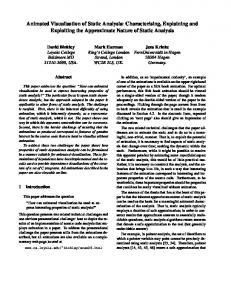
We designed VlUM so that the user model might be explored in conjunction with an associated activity. Accordingly, the VlUM visualisation exists in a vertical segment of the screen about 350×600 pixels in size, leaving room for a web page to be displayed in full to its right. While a user may wish to focus on the attributes of a single component of the user model, they will often wish to still see the ‘context’, including related components. VlUM takes this to an extreme, showing all components at all times, but with emphasis on the current component of interest and its peers, a visualisation technique known as ‘focus+context’ [8, 6, 10]. For example, in Figure 1, which shows a user model from a medical domain, the currently selected component is Effect of infection on pregnancy (role of placenta). This title is in a larger font, and has more space around it. Related titles, which are peers of the current selection in the model graph, are shown in a slightly smaller font and with less space. An example would be Functions of the heart as a pump. This regression in font size and spacing continues through the graph, and so the topics most distant from the current selection are crowded together and small. A slider above the main pane enables the user to set the standard required to assess a component of the model as true. In the spirit of user control, this means users can determine the boundary between the classification of a component as true (displayed as green) or false (red). The saturation of the colour indicates degree. The current selection in Figure 1 is very red, indicating that the user is not doing well in that topic. We considered it important that a the user have the means to adjust this standard for assessing the data in a user model. For instance, in a medical course, a student should have the freedom to define their pass standard at a high standard if they wish. In that case, a component would appear in green only if the system had strong evidence that the user knew that aspect. Equally interestingly, the user could set the standard very low. In that case, the only red components would be those for which the system had strong evidence that the user did not know the aspect. These would indicate areas the student might work on first. Similarly, where the model is displaying predicted user preferences, the
VlUM, Visualising Large User Models
3
Fig. 1. The visualisation in VlUM.
user should be able to set a high standard in order to see just the most highly recommended components. The ‘certainty’ attribute of a component is shown by the x offset of the title from the left of the display. The current selection in Figure 1 is not certain of its value. If a component has no data, it is coloured yellow. If a user is given VlUM in the state shown in Figure 1, and clicks on Effect of virus on host cells which is slightly above Effect of infection on pregnancy (role of placenta), VlUM will change (with animation) to the state shown in the right image of Figure 2. The graph now has Effect of virus on host cells at the root, and Effect of infection on pregnancy (role of placenta) at a lower depth. Since the distance between the topics in the graph has not changed, the sizes of the two components are essentially swapped. However, the relative positions of the components on the display will change to reflect the new spanning tree of the graph. Titles are not fixed to any particular position, but move as the
4
James Uther, Judy Kay
Fig. 2. Two steps in use of the model visualisation. The viewer starts as seen on the left. The focus component is Effect of infection in pregnancy. Topics which most closely related to this have more space around them and so are more visible. For example, slightly above it is Effect of virus on host cells. Clicking on it alters the display to that on the right.
spanning tree causes ‘warping’ of the display surface, but as already mentioned, the components are always displayed in the order they appear in the model file. There are three menus. These enable a range of functions which are irrelevant for this paper. A working demonstration of VlUM may be found at http://www. it.usyd.edu.au/~jimu/vlum/.
3
User Study
We designed the evaluation experiment in terms of a user model for preferences for movies, using data from the Internet Movie Database (IMDB)1 . Essentially, the model represented the system’s model of a user’s preferences for a collection of movies. We chose this because it provided a highly understandable domain. We felt that users should be easily able to interpret requests to do tasks of the form: – find a recommendation for a movie the user is predicted to like; 1
http://www.imdb.org/
VlUM, Visualising Large User Models
5
– find a recommendation for a movie that the user is predicted to dislike. The full experiment explored other aspects but this paper focuses on the utility of the visualisation to assist users in answering these core questions. For full detail, see [12]. The IMDB domain allowed us to select participants from a variety of backgrounds. Participants were included computer science undergraduate and postgraduate students, academic and administrative staff, as well as other members of the public. Ages ranged from 19 to 53. Sessions were completed at different times within a one week period. Participants were provided with the running program. They were asked to work through the directions provided by the system. They were informed that their activity would be logged. Then they were left alone to complete the automated tutorial about VlUM and then work through the experimental session. We did want the participants to feel pressured by our presence. Broadly, the experiment explored how well users would be able to explore a user model to answer questions such as those posed in Section 1. All users in our experiment were asked to do the same set of tasks on the same model, created for a hypothetical user. This improved the comparability of the results and focused on the evaluation of the power of the visualisation for a large user model. We wanted to assess whether VlUM could be used effectively for large user models. So we created a user model with 700 components, and then progressively stripped this model to give four models of 100, 300, 500 and 700 components. These sizes were chosen to give a good range of data sizes, starting at slightly more titles than the previous work [5]. We chose the upper value of 700 as we believed that was an ambitious upper limit and we expected that the visualisation would probably be less effective, with users taking longer to explore models of this size and we anticipated users would make more mistakes at this model size. It was also slightly larger than the number of topics in one of our development domains, a model of medical knowledge for a full medical degree programme. That range was divided to give our four data set sizes, as we expected this to help us see the trend in the performance of the visualisation as the number of components increases. We refer to the task of finding parts of the model based on their score as ‘task rec’, for ‘recommend’. In this, the participant must select a title with a score of a given value (>80%, for example). To accomplish this, the user must first set the slider to the required value. Then the visualisation shows titles in green only if the recommendation score is above this value. The rest of the titles appear in red or yellow. The user’s task is to find a title that is still green (recommended). As the user moves the mouse over a title, it turns white, with its score and certainty shown at the bottom of the display. The user completes the task by clicking on the title chosen. In the tutorial the user was asked to find a movie with a recommendation of < 40%. In the experiment, there were two such questions, one asking for a movie with a recommendation of > 80%, and one of < 30%.
6
James Uther, Judy Kay
With VlUM the task of finding a recommendation can be accomplished once the user had learned the use of the slider. At that point, the user needs to scan the user model overview, looking for the green indicating a recommendation and then using the mouse, first to put over a title to check exact details of an intended selection, and then to select it. All participants worked with the 300 item data set for an initial online tutorial. After the tutorial, users performed experimental tasks with a randomly selected set for the main test. Of the 57 participants, 10 received the 100 item set in the main test, 14 received the 300, 14 the 500 and 18 the 700 item set. Most user actions, including the times that questions were displayed to the user, were logged, and the logs saved to a server for later analysis. 3.1
Analysis and Results
We analysed the time to answer each question, whether the question was answered correctly, and how many steps it took to answer the question. We now report each of these. The table to the right summarises Data set average number of number of the average times taken. Note that Size time tasks users this time is measured from the mo300T 42.4 57 57 ment the question was presented to 100 21.0 20 10 the time the user clicked on their fi300 21.2 28 14 nal answer and moved on to the next 500 31.2 28 14 task. So, it includes time to read and 700 42.7 36 18 comprehend the question. The ‘300T’ row in the table is for the tutorial. Since all participants performed the tutorial, the first row includes all participants. There was one task of this type in the tutorial and two in the main test. This is why the number of test tasks is double the number of users. It can be seen that the average time for the task improved markedly from the tutorial to the two test tasks in all but the 700 element data set. The two smaller data set sizes appear to have similar times while the 500 element dataset appears to take longer and the 700 element set longer again. Figure 3(a) shows the distribution of times taken. The data set size is on the x axis and time in seconds on the y. To make the graphs more meaningful, points that were more than ten times the set average were declared outliers. These are shown as ol values at the top of each set of results. There were no such values for the smaller data sets, one for the 500 element dataset and two for the 700 element set. All correct answers appear as bullets (•)and incorrect answers as delta (∆). The average of the correct points is shown as a dotted line, and one standard deviation from that average as horizontal marks. The vertical lines at each data set size show the range of the first and third quartile of the set of correct answers. The number of correct and incorrect answers for each data set size is indicated towards the top of the graph. There were 16 correct answers plotted for the 100 item data set, 4 incorrect answers, and no outliers.
VlUM, Visualising Large User Models
rec • 16 ∆4 ol 0
150
•
• 24 ∆4 ol 0
200 •
• • 25 ∆2 ol 1
•∆
• 19 ∆15 ol 2
150
∆
100 50 0
•• ••∆ ••• •••∆∆ •
100
300
• ••• •• •• ••••• • ••∆ •∆
•• •• ••∆∆∆ ••• •∆ ∆ ∆ ••∆ ∆∆ ∆
500 Data set size
∆19 ol 3
100
•∆ •
•• • • ••• ••••• ••••∆ •∆∆
rectutorial • 35
Time to answer (sec)
Time to answer (sec)
200
50 0
700
rec • 24
∆4 ol 0
• • •
7
•
• •• ∆ ∆ • •• •• ∆ • •••∆ •• ••∆∆∆∆∆ •••••∆∆∆∆ ••• ∆∆∆ •••••∆∆
•• •
tutorial
main
• • ••• • • ••• •••••• ∆ •• ∆∆ ∆
(b) Comparison for the 300 item set between the tutorial and the experiment.
(a) Distributions of times to complete in the experiment.
Fig. 3. Times to complete the task in tutorial and experiment.
Figure 3(b) shows the comparison with the 300 item data set in both the tutorial and the test itself. This shows the distribution of the average results in the table above, with a larger proportion of users answering correctly and more quickly in the test, compared with the tutorial. We now explore the accuracy of the answers. Figure 4 Size avg % n shows how often participants correctly answered the task. 300T 65 57 The data is summarised in the table on the right. The data is 100 80 20 plotted with data set size on the x axis and percent correct on 300 86 28 the y. The number of points used in this average is indicated 500 93 28 at the bottom of the graph for each data set size. There were 700 53 36 20 answers for the 100 item data set, with 80% answered correctly. The accuracy peaked at 500 items with 93% correct over 28 trials. rec
100
Percent Correct
80 60 40 20 0
• 20
100
• 28
300
• 28
500 Data set size
• 36
700
Fig. 4. Percentage of correct answers for task.
8
James Uther, Judy Kay
We now explore the number of steps users took to do each task. This indicates how much participants needed to work to find the answer. The fewer steps, the more efficiently the participant answered the question. A ‘step’ is a click, a search, or using the slider, where one ‘step’ is counted if the slider is used while answering the question. Size steps n The raw data is shown in Figure 5 and summarised in the table to the right. The data set size appears on the x axis 300T 2.1 57 and number of steps taken on the y. Outliers were removed 100 2.4 20 where a user took more than five times the average and the 300 2.3 28 number of these is shown as ‘ol’. Correct answers are shown 500 3.0 28 as bullets (•), and incorrect as a delta (∆). The average of the 700 4.8 36 correct answers is plotted as a dotted line, and one standard deviation from that average as horizontal marks. The number of correct and incorrect answers in each data set used in the plot is indicated toward the top of the graph. For example, for the 100 item data set, there were 16 correct and 4 incorrect answers and users took an average of 2.4 steps to answer the task correctly, with a small deviation of about 0.2 steps.
• 16
Steps to answer
8 •
6
∆
0
∆4 ol 0
•
•
4 2
rec
•
••∆ ••∆ ••
100
• • •• •••∆• •∆∆
300
•
• 24
∆4 ol 0
10
• • 25
• 16
∆2
ol 1 • •• •• •• ••∆ • •
500 Data set size
∆∆
∆17 ol 3
• • • ∆ • ••∆ •∆ ∆ ••∆ •∆∆ ∆
700
(a) Steps to correctly complete rec.
8 Steps to answer
10
• 37 ∆20 ol 0
rectutorial •
∆
• ∆∆
6 4 2 0
• 24 ∆4 ol 0
rec
•
• • •• • ∆ •• •••••∆∆∆ •• ••••••∆•∆∆∆∆∆∆∆ •••• •∆
•• • •• • •• • •••• ∆ ••• •∆∆
tutorial
main
(b) Comparison between steps taken in tutorial and experiment
Fig. 5. Steps to answer task rec in the tutorial, and in the experiment proper.
Figure 5(b) shows that in the tutorial many steps were taken to do the task, and often incorrectly. By comparison, there was completed with less steps and more accurate answers. We now report the correctness performance in the tutorial compared with the experiment. We analysed this for two reasons. First, we wanted to determine whether the tutorial appeared to provide enough help for most users to know how to do the task. Secondly, we wanted to see if there were interesting cases which would improve our understanding of the above data. For example, users
VlUM, Visualising Large User Models
9
who performed well on the tutorial but poorly in the experiment, might suggest that size of the experimental data set was the problem. The table to the right shows how often questions in both T1 E1 E2 Σ tutorial and experiment were answered correctly or otherwise. • • • 29 The first row indicates that 29 users gave correct answers for • 7 the tutorial and both experiment questions. The next row in• • 6 dicates 7 users had wrong answers in the tutorial but correct • • 6 answers for the first experimental task and wrong answers for 5 the second. One trial was removed from the table because not • 1 all relevant questions were answered. The table indicates that • 1 most users did at least as well on one experimental task as on • • 1 the tutorial and there were several users who failed on the tutorial task but nevertheless were able to do at least one experimental task correctly: 7 of these doing just E1 correctly, 6 doing both experimental task correctly and one doing E2 correctly. Just one user did the tutorial correctly and then failed to do either experimental task correctly. It seemed that the tutorial was a good preparation for the task. Figure 3(b) supports this, with the time to answer the task dropping between the tutorial and the main test.
4
Summary and Conclusion
The task was answered well for smaller data sets. At 100 items it took 21 seconds to answer correctly, which was done about 80% of the time. Although it was still answered correctly more than 90% of the time up to 500 items, it took longer as the size increased. In particular, the number of steps taken by some participants to find a correct answer increased markedly with data set size, as shown in Figure 5(a). It seems that hunting for the correct answer in an increasingly cluttered display took its toll. At 500 items it was taking around 30 seconds to answer correctly. At 700 items the percentage of correct answers dropped to 53%, again suggesting a limit to the amount of data that can be displayed if this task is to be possible for novices. In summary, the task was correctly answered most of the time within 35 seconds for data sets up to 500 items. At 700 items the time to answer rose somewhat, the accuracy dropped, and the steps required to find a correct answer rose more than linearly as 700 items was approached. This suggests that at extremely large model sizes the cluttering of the ‘unfocused’ items does slow users finding items of a given level of recommendation. It should be noted, however, that these sizes are more than seven times larger than the number of items displayed by previous tools. There are strong reasons for offering an overview of a user model. VlUM is a new visualisation, which was developed for the purpose of providing such an overview. It aims to allow a user to find interesting features of a large model. It exploits relationships between the components of a user model to control the parts which are most visible at any point in time. It enables users to identify the true components within a large model, since these can be seen as the green strings
10
James Uther, Judy Kay
in the display. Similarly, it enables users to see the false components, as the red strings in the visualisation. We have described an evaluation which indicates that most users were able to find such components even when 700 components were displayed. Moreover, users were able to do this task quite quickly with up to 500 components.
References 1. J. Bertin. Graphics and Graphic Information Processing, pages 62–81. 1981. 2. S Bull, P Brna, and H Pain. Extending the scope of the student model. User Modeling and User-Adapted Interaction, 5(1):44–65, 1995. 3. Susan Bull and P Brna. What does Susan know that Paul doesn’t? (and viceversa): contributing to each other’s student model. In B de Boulay and R Mizoguchi, editors, International Conference on Artificial Intelligence in Education, pages 568–570. IOS Press, 1997. 4. I. Herman, G. Melan¸con, and M. S. Marshall. Graph visualisation and navigation in information visualisation, 1999. 5. J Kay. A scrutable user modelling shell for user-adapted interaction. PhD thesis, University of Sydney, 1999. 6. J. Lamping and R. Rao. The hyperbolic browser: A focus + context technique for visualizing large heirarchies. Journal of Visual Languages and Computing, 7(1):33– 55, 1996. 7. Ora Lassila and Ralph Swick. Resource description framework (RDF) model and syntax specification, 1999. 8. Y. K. Leung and M. D. Apperley. A review and taxonomy of distortion-orientation presentation techniques. ACM Transactions on Computer-Human Interaction, 1:126–160, 1994. 9. A. Paiva, J. Self, and R. Hartley. Externalising learner models. In J. Greer, editor, Proceedings of the World Conference on Artificial Intelligence in Education, Washington DC, U.S.A., 1995. AACE. 10. R. Rao and Stewart K. Card. The table lens: Merging graphical and symbolic representations in an interactive focus + context visualization for tabular information. In Proceedings CHI’94, pages 318–332, 1994. 11. J Self. Bypassing the intractable problem of student modelling: Invited paper. In Proceedings of the 1st International Conference on Intelligent Tutoring Systems, pages 18–24, Montreal, 1988. 12. James Uther. On the visualisation of large user models in web based systems. PhD thesis, University of Sydney, 2001. 13. J. D. Zapata-Rivera and J. Greer. Inspecting and visualizing distributed bayesian student models. In G Gauthier, C Frasson, and K VanLehn, editors, Intelligent Tutoring Systems ITS 2000, pages 544–553, Montreal, June 2000. 14. J. D. Zapata-Rivera and J. Greer. Externalising learner modelling representations. In Proceedings of the Workshop on External representations in AIED: Multiple forms and multiple roles, held with the 10th International Conference on Artificial Intelligence in Education (AI-ED), 2001. 15. J. D. Zapata-Rivera and J Greer. Exploring various guidance mechanisms to support interaction with inspectable learner models. Intelligent Tutoring Systems, pages 442–452, 2002.