Volatility Filters for Asset Management: An Application to ... - CiteSeerX

Volatility Filters for Asset Management: An Application to Managed Futures By Christian L. Dunis∗ and Jia Miao∗∗ (Liverpool John Moores University and CIBEF∗∗∗) January 2005

Abstract Technical trading rules are known to perform poorly in periods when volatility is high. The objective of this paper is to study whether addition of volatility filters can improve model performance. Different from previous studies on technical trading rules which base their findings from an academic perspective, this paper tries to relate to the real world business: two portfolios, which are highly correlated with a managed futures index and a currency traders’ benchmark index are formed to replicate the performance of the typical managed futures and managed currency funds. The volatility filters proposed are then applied directly to these two portfolios with the hope that proposed techniques will then have both academic and industrial significance. Two volatility filters are proposed, namely a “no-trade” filter where all market positions are closed in volatile periods, and a “reverse” filter where signals from a simple Moving Average Convergence and Divergence (MACD) are reversed if market volatility is higher than a given threshold. To assess the consistency of model performance, the whole period (04/01/1999 to 31/12/2004) is split into 3 sub-periods. Our results show that the addition of the two volatility filters adds value to the models performance in terms of annualised return, maximum drawdown, risk-adjusted Sharpe ratio and Calmar ratio in all the 3 sub-periods. Keywords: managed futures, active asset management, technical rules, confirmation filter, volatility filter.

∗

Christian Dunis is Professor of Banking and Finance at Liverpool John Moores University and Director of CIBEF (E-mail: [email protected]) ∗∗ Jia Miao is an Associate Researcher with CIBEF and currently working on his PhD thesis at Liverpool John Moores University (E-mail: [email protected]) ∗∗∗ CIBEF – Centre for International Banking, Economics and Finance, JMU, John Foster Building, 98 Mount Pleasant, Liverpool L3 5UZ.

1 of 14

1. Introduction. Financial forecasting has always been a main focus of the financial and economic literature. Many articles proposing numerous simple or more sophisticated forecasting techniques have claimed that a trading strategy based on their forecasts can outperform that of a buy-and-hold strategy or some other benchmark forecasting techniques. These trading strategies usually require the underlying assets to be traded actively, while in practice trading on a high-frequency basis in some markets is not feasible simply because of transaction costs. In markets like the stock and bond cash markets, the benefits from switching market positions at high frequency can hardly compensate for the transaction costs incurred. It is well known that transaction costs in most futures markets and foreign exchange (FX) cash markets are much lower compared to other financial markets. The low transaction costs along with the ability to “go short” easily in these markets make it possible to profit from active trading strategies. As a matter of fact, the managed futures and managed currency traders are the most active market players. The motivation for this paper is twofold. Firstly, although the majority of such active fund managers rely their trading strategies on technical trading rules, these rules are known to perform poorly in periods when volatility is high. Therefore this paper studies whether the addition of a confirmation filter, based on the underlying market volatility, can help to improve model performance. Secondly, despite the fact that technical trading rules have been extensively studied, most of these articles build their findings from an academic perspective, while few of them relate their results to the real world of investment. This paper tries to relate our findings to the real business world by forming two portfolios that are highly correlated with a managed futures index and a currency traders’ benchmark index, and which replicate the performance of the typical managed futures and managed currency funds. The proposed techniques are expected to have both the academic and industrial significance. Of the two portfolios formed, the futures portfolio is highly correlated with the CSFB/Tremont Managed Futures index and is built to mimic the performance of typical managed futures funds. Following Lequeux and Acar (1998) who create a dynamic currency futures index (AFX), we also form an FX portfolio using the 9 most heavily traded FX spot rates replicating average currency managers. What is more, the specifications of the Moving Average Convergence and Divergence (MACD) used in the two dynamic portfolios are the ones applied by Lequeux and Acar (1998) for the theoretical reasons that they explained instead of any other number selected arbitrarily. Two volatility filters are proposed, namely a “no-trade” filter where all market positions are closed in volatile periods, and a “reverse” filter where signals from a simple MACD are 2 of 14

reversed if the market volatility is higher than a given threshold. Our results show that the addition of the two volatility filters adds value to the portfolios performance in terms of annualised return, maximum drawdown, risk-adjusted Sharpe ratio and Calmar ratio in all the 3 sub-periods. As for the two filters applied, the “reverse” strategy seems to outperform the “no-trade” strategy for most performance measures most of time. The paper is organized as follows: section 2 presents a brief review of the relevant literature, section 3 explains the methodology and section 3 describes the data used. Section 5 presents our empirical results, focusing on the models performance during different sub-periods, followed by concluding remarks in section 6. 2. Literature Review The results from literature about the profitability of technical trading rules are conflicting. Much of the earlier work1 concludes that it is not possible to outperform the market using technical trading rules. However Brock et al. (1992) provide strong support for technical strategies, with returns from their technical trading strategies outperforming four popular null models: the random walk, the AR(1), the GARCH-M and the EGARCH. Blume et al. (1994) show that the sequence of data for both past prices and trading volume improve the predictability of equity returns within the “noisy rational expectation” framework. Kwon and Kish (2002) find that technical trading rules add value to capture profit opportunities over a buy-and-hold strategy. Sullivan et al. (1999) show however that the results of Brock et al. (1992) are substantially weakened when the survivorship bias is corrected, and Ready (2002) argues that the apparent success of the Brock et al. (1992) moving average rules is a spurious result of datasnooping. Despite the academic controversy over the merits of technical trading rules, it is one of the most widely used forecasting techniques among market practitioners as mentioned by Billlingsley and Chance (1996) who note that 70% of the Commodity Trading Advisors (CTAs) are trend followers and tend to trade in a similar manner. The heavy use of technical trading rules by futures and currency funds has also been documented from a technical perspective. For instance, Jensen (2003) replicates, with a 75% correlation, the typical managed-futures hedge fund (represented by the CSFB/Tremont managed futures index) with a basic 1-month and 3-month moving average trading strategy applied to the major futures markets. Lequeux and Acar (1998) form a dynamic currency index (AFX), based on the performance of 3 simple moving averages, that exhibit similar performances to currency traders’ benchmarks.

1

See, for instance, Alexander (1961) and Fama and Blume (1966).

3 of 14

The market volatility has an impact on futures trading, for instance, Pan et al. (2003) study the influence of volatility on futures trading and find that an increase in volatility motivates traders to engage in more trading in futures markets. On the other hand, volatility filters have been proposed to improve the overall performance of trend-following systems because trend-following systems are known to perform poorly when markets become volatile. Roche and Rockinger (2003) explain that high volatility periods often correlate with periods when prices change direction, and therefore proposed to reverse the technical signals generated when market volatility is forecast to be higher than a chosen threshold. Dunis and Chen (2005) argue that MACD models perform poorly in volatile markets, precisely because volatile markets imply frequent direction changes, and thus introduce a volatility filter which stops trading at times of high volatility. 3. Technical Trading Rules: the Methodology 3.1 MACD Technical trading rules have long been applied in financial markets, and these rules are still one of the most popular techniques applied by market practitioners. A technical trending system is built based on the basic assumption that “everything is in the rate and the market moves in trend”. Then the major task of such a trend-following system is to define the prevailing trend and to identify early reversals. One of the most widely used technical trending systems is the moving average convergence and divergence system (MACD). An MACD crossover system consists of two moving averages (MA), a short-term MA and a long-term MA, of the underlying financial series. For the daily data, we use “s D / l D” to refer to a specific MACD, where s and l is the number of days in the short-term and long-term MA respectively, while for the monthly it is “s M / l M” accordingly. In such a system, the long-term MA is to identify the prevailing trend, and the short-term functions as the market timing device. The trading strategy based on an MACD system is to go long (or short) when the short-term MA is above (or below) the long-term MA. The idea behind MAs is to smooth out a volatile time series and there are many ways to compute MAs. We use the simple MA where all past observations are assigned equal weights as: n

MA( t ) = (1 / n)∑ pt −i i =0

3.2 Trend-following technique and market volatility In our study, we use the time-varying RiskMetrics volatility model to measure the conditional market volatility and amend our trend-following models when a given level of conditional volatility has been breached. RiskMetrics was developed by JP Morgan (1994) for the measurement, management and control of market risks in its trading, arbitrage and 4 of 14

own investment account activities. The RiskMetrics volatility can be seen as a special case of Bollerslev (1986) GARCH model with pre-determined decay parameters, and it is calculated using the following formula:

σ 2 (t +1 / t ) = µ * σ 2 (t / t −1) + (1 − µ ) * r 2 (t ) where σ 2 is the volatility forecast of a specific asset, r 2 is the squared return of that asset, and µ = 0.94 for daily data and 0.97 for monthly data as computed in JP Morgan (1994). 3.3 Filter Rules In this article, we use the symbol MA(p) (t+1,t) to denote the trading signals from an MACD model at time t for time t+1, where p is the volatility filter imposed on that model: p takes the value of 0 if there is no volatility filter, it takes the value of 1 when the “no-trade” filter is used and 2 when a “reverse” filter is in use. 3.3.1 “No-trade” Strategy Since the MACD is found to perform poorly in volatile markets, following Dunis and Chen (2005) the first filter rule is simply to stay out of the market when the underlying volatility is forecast to be higher than a certain threshold T. The previous MACD trading rules are thus combined with the “no-trade” strategy: MA(0) (t+1,t)

σ 2(t+1,t) < T

0

σ 2(t+1,t) > T

MA(1) (t+1,t) =

3.3.2 “Reverse” Strategy When a market experiences high volatility, Dunis and Miao (2005) find that the returns generated from the original MACD signals become negative most of the time. Roche and Rockinger (2003) explain that high volatility periods often correlate with periods when prices change direction, and therefore proposed to reverse the signals generated when market volatility is forecast to be higher than a chosen threshold. We use this strategy as the second filter to our MACD system: MA(0) (t+1,t)

σ 2(t+1,t) < T

- ( MA(0) (t+1,t) )

σ 2(t+1,t) > T

MA(2) (t+1,t) =

4. Data and Dynamic Portfolios

The entire sample period is from 02/01/1998 to 31/12/2004 (1814 observations for daily data and 84 observations for monthly data) and all datasets used are daily and monthly 5 of 14

closing prices obtained from Datastream2. We use data of the first year of the databank for MACD calculation and volatility measurement initialisation, and we just select those MACD parameters that are popular in the market without making the effort to use a lot of “in-sample” data to optimise model parameters, the whole period for performance measurement purposes is from 04/01/1999 to 30/07/2004 (1556 observations for daily data and 72 observations for monthly data). To measure the consistency of those performance measures, we further split the performance period into 3 sub-periods: i.e. a 6-year period (04/01/1999-31/12/2004), a 4-year period (02/01/2001-31/12/2004) and a 2-year period (02/01/2003-31/12/2004). The daily (monthly) asset returns r in time period t+1 are calculated as the percentage change of the daily (monthly) closing value p: rt +1 = (

pt +1 − pt ) pt

4.1 Futures Portfolio The major objective of this paper is to apply volatility filters to two portfolios that replicate the performance of average futures and currency traders. Jensen (2003) replicates the typical managed futures hedge fund with a basic 1-month by 3-month moving average trading strategy applied to Eurdollar (EUR$), S&P500, US T-note, EUR/USD and USD/JPY futures markets, while in this paper we add two more assets, GBP/USD and Copper to expand the asset coverage while at the same time retaining a high correlation level. The contracts included in the futures portfolio are EUR$ (CME), T-Note (CBT), S&P500 (CME), EUR/USD (CME), USD/JPY (CME), GBP/USD (CME) and Copper (COMEX) as shown in table 4.1 below3. The 7 futures assets are U.S contracts with reasonably similar closing times. The equally weighted portfolio has been constructed on a trial and error basis to highly correlate with the CSFB/Tremont managed futures performance index. For daily data, the MACD specifications are those MACDs that are widely used by market practitioners. The futures portfolio formed in this way is highly correlated with the CSFB/Tremont managed futures index. Calculated from January 1994, the CSFB/Tremont hedge fund index is the industry’s leading asset-weighted hedge fund index. There are also 10 sub-indices that represent the performance of the 10 primary hedge fund subcategories 2

Since the EUR/USD exchange rate only exists from 04/01/1999, we follow the approach of Dunis and Williams (2002) to apply a synthetic EUR/USD series from 02/01/1998 to 31/12/1998 combining the spot USD/DEM and the fixed EUR/DEM exchange rate. The synthetic EUR/GPB, EUR/JPY and EUR/CHF are created following the same approach. 3 CME stands for Chicago Mercantile Exchange, CBT stands for Chicago Board of Trade and COMEX stands for Commodity Exchange, New York.

6 of 14

Asset Allocation and Dynamic MACD strategy for the Futures Portfolio

Table 4.1

EUR$

T-Note

(CME)

(CBT)

(CME)

(CME)

(CME)

(CME)

(COMEX)

14.29%

14.29%

14.29%

14.29%

14.29%

14.29%

14.29%

1D / 250D 1D / 250D 3D / 250D 1D / 61D

1D / 61D

1D / 61D 1D / 250D

1M / 12M 1M / 12M 1M / 12M

1M / 3M

1M / 3M

Assets (Futures) Weights MACD Strategy (daily data) MACD Strategy (monthly data)

S&P500 EUR/USD USD/JPY GBP/USD

1M / 3M

Copper

1M / 12M

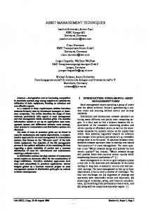
based on their investment style. CSFB/Tremont analyzes the percentage of assets invested in each subcategory and selects funds for the index based on those percentages. For our purpose here, we analyse the CSFB/Tremont managed futures sub-index. Since all CSFB/Tremont indices are computed on a monthly basis, we also use monthly data with monthly MACD specifications. Bearing in mind that the lowest time span with monthly data will be 1 month, we try to replicate the time span of the daily MACD for the longer term moving average: for instance, a 1D/61D daily MACD for the EUR/USD series is approximated by a 1M/3M monthly MACD. Daily and monthly MACD specifications as well as asset allocation weights for the futures portfolio can be found in table 4.1. With this approach, both the daily and monthly dynamic futures portfolios are highly correlated with the CSFB/Tremont managed futures index for the 6-year, 4-year and 2-year periods. This futures portfolio is then able to replicate the typical managed futures funds in the market (see Figure 4.1). Figure 4.1 Correlation between CSFB/Tremont Managed Futures Index and the Futures Portfolios CSFB/Trem ont Managed Futures Index Futures Dynam ic Portfolio w ith Daily Data

15.00%

Futures Dynam ic Portfolio w ith Monthly Data

10.00% 5.00% 0.00% -5.00% -10.00% Dec-04

Jun-04

Dec-03

Jun-03

Dec-02

Jun-02

Dec-01

Jun-01

Dec-00

Jun-00

Dec-99

Jun-99

Dec-98

7 of 14

Table 4.2 below suggests consistency across the different periods under review4. The fact that the dynamic portfolio represents the performance of managed futures funds is not only supported by its consistent and high correlation to the CSFB/Tremont managed futures index correctly over time. It is also confirmed by the closeness of both risk-adjusted Sharpe ratios (see table 5.1 below), even if the dynamic portfolio has a lower return and a lower volatility compared to the CSFB/Tremont index, but this is due to the fact that most futures funds are leveraged. Table 4.2

Correlation with CSFB/Tremont Managed Futures Index 6-year Period

4-year Period

2-year Period

Futures Portfolio (daily data)

0.68

0.71

0.64

Futures Portfolio (monthly data)

0.62

0.69

0.58

4.2 Currency Portfolio Lequeux and Acar (1998) introduce a dynamic currency index (AFX index) to replicate the performance of the typical currency fund managers. The index consists of 7 currency futures rates using 3 simple MACD (namely 1D/32D, 1D/61D and 1D/117D) strategies with each MACD taking the same weight in generating trading signals. They found that the AFX index has high correlation with and low tracking error to currency traders’ performance. Following the same 1D/32D, 1D/61 and 1D/117D MACD combination strategy, we form the FX portfolio using currency spot rates since trading volumes in the FX spot market are much bigger than those in the futures market. We also expand the portfolio composition to 9 currency rates and update the portfolio weighting scheme using the most recent BIS trading volume survey (BIS 2004). Both the asset combination and weights of the FX portfolio are shown in Table 4.3. Table 4.3 Currency

Weights

FX Portfolio Currency Allocation USD

GBP

EUR

USD

USD

AUD

EUR

EUR

EUR

/JPY

/USD

/USD

/CHF

/CAD

/USD

/GPB

/JPY

/CHF

21.13%

17.49%

35.76%

5.57%

5.07%

6.42%

3.07%

3.64%

1.86%

5. Empirical Results

5.1 Risk-Adjusted Performance Measures

4

Since the CSFB/Tremont index is only available on a monthly basis, we transform the daily performance of the portfolio into monthly performance, and the correlation is then calculated between the two monthly series.

8 of 14

Higher returns are usually associated with higher risks, and a model’s performance will be biased if assessed merely on the basis of return. Therefore in addition to the measure of yield, in terms of the cumulative and annualised return, and risk exposed, in terms of annualised volatility and maximum drawdown, we also use risk-adjusted measures to asset model performance. The Sharpe ratio is perhaps the best known risk-adjusted statistic introduced by Sharpe (1966)5 as: Sharpe ratio =

Annualised return Annualised volatility

Within the Sharpe Ratio definition, risk is measured as the volatility of the market, and both upside and downside volatility are penalised. In reality, a fund manager is only concerned with the downside risk. The Calmar ratio was created to address this concern (Jones and Baehr 2003). Calmar ratio =

Annualised return Maximum drawdown

With the Calmar ratio, market risk exposed is measured by the maximum downside risk an investor can suffer if he enters the market at the worst time. n ⎡ ⎤ Maximum drawdown = Min ⎢ rt − Max ( ∑ rt )⎥ t =1 ⎣ ⎦

The entire performance period for both the futures and FX portfolio is further split into 3 sub-periods to measure the consistency of the trading performance over different periods of time. Model performance statistics for the 2 portfolios can be found in table 5.1. 5.2 Results for the Futures portfolios Not only does the futures portfolio with the dynamic daily MACD strategy highly correlate with the CSFB/Tremont managed futures index, but it also produces similar Sharpe ratios to those from the index for all the 3 sub-periods, which confirms that this portfolio can consistently replicate the performance of the typical managed futures funds. For the futures portfolio with daily data, the addition of either the “no-trade” or the “reverse” filters brings a significant improvement in terms of annualized return and risk-adjusted measures like the Sharpe and Calmar ratio in all the 3 sub-periods. In the longer term 6-year period, the “reverse” strategy increases the annualized return from 3.06% to 5.47%, while on the other hand the “no-trade” strategy lowers the maximum drawdown successfully with improving the annualized return at the same time. More such significant improvements on major performance measures are also found over the 4-year and 2-year sub-periods. The 5

In its original version, the numerator of Sharpe ratio is defined as the investment return less the risk-free rate of return in the same period. Since in this paper the Sharpe ratio is used as a criterion to measure relative model performance, for simplicity we omit the risk-free rates in all Sharpe ratio calculations.

9 of 14

Table 5.1

Model Performance Measures

futures portfolio performance (daily data) Correlation to CSFB/Tremont Annualised Return Cumulative Return Annualised Volatility Maximum Drawdown Sharpe Ratio Calmar Ratio

6-year Period (04/01/99-31/12/04)

4-year Period (02/01/01-31/12/04)

2-year Period (02/01/03-31/12/04)

CSFB/ futures "no-trade" “reverse” Tremont portfolio filter filter

CSFB/ futures "no-trade" “reverse” Tremont portfolio filter filter

CSFB/ futures "no-trade" “reverse” Tremont portfolio filter filter

1 0.68 6.97% 3.06% 41.82% 18.38% 12.51% 5.74% -14.69% -6.59% 0.56 0.53 0.47 0.46

1 0.71 10.37% 4.13% 41.47% 16.54% 13.47% 6.60% -14.69% -6.59% 0.77 0.63 0.71 0.63

1 0.64 10.40% 5.77% 20.80% 11.54% 13.32% 6.48% -14.69% -6.59% 0.78 0.89 0.71 0.88

0.69 4.26% 25.59% 5.53% -5.53% 0.77 0.77

0.67 5.47% 32.79% 5.51% -4.88% 0.99 1.12

futures portfolio performance CSFB/ futures "no-trade" “reverse” Tremont portfolio filter filter (monthly data) Correlation to CSFB/Tremont Annualised Return Cumulative Return Annualised Volatility Maximum Drawdown Sharpe Ratio Calmar Ratio

1 0.62 6.97% 3.42% 41.82% 20.54% 12.51% 5.26% -14.69% -7.89% 0.56 0.65 0.47 0.43

0.59 3.94% 23.62% 5.06% -7.89% 0.78 0.50

0.52 4.45% 26.70% 5.15% -7.89% 0.86 0.56

0.73 5.53% 22.12% 6.32% -5.53% 0.88 1.00

0.72 6.93% 27.71% 6.22% -4.88% 1.11 1.42

0.63 6.57% 13.14% 6.28% -5.37% 1.05 1.22

0.62 7.37% 14.73% 6.18% -4.85% 1.19 1.52

CSFB/ futures "no-trade" “reverse” Tremont portfolio filter filter

CSFB/ futures "no-trade" “reverse” Tremont portfolio filter filter

1 0.69 10.37% 4.71% 41.47% 18.83% 13.47% 5.86% -14.69% -7.89% 0.77 0.80 0.71 0.60

1 0.58 10.40% 5.31% 20.80% 10.63% 13.32% 5.93% -14.69% -4.62% 0.78 0.90 0.71 1.15

0.67 4.75% 18.99% 5.57% -7.89% 0.85 0.60

0.62 4.79% 19.15% 5.64% -7.89% 0.85 0.61

0.53 5.39% 10.79% 5.34% -3.26% 1.01 1.66

0.41 5.47% 10.95% 5.48% -2.81% 1.00 1.95

currency portfolio performance (daily data)

currency portfolio

"no-trade" filter

reverse filter

currency portfolio

"no-trade" filter

reverse filter

currency portfolio

"no-trade" filter

reverse filter

Annualised Return Cumulative Return Annualised Volatility Maximum Drawdown Sharpe Ratio Calmar Ratio

1.60% 9.90% 5.62% -14.09% 0.29 0.11

3.12% 19.24% 4.81% -11.70% 0.65 0.27

4.63% 28.59% 5.00% -9.30% 0.93 0.50

0.57% 2.37% 5.59% -14.09% 0.10 0.04

2.37% 9.77% 4.88% -11.70% 0.48 0.20

4.16% 17.17% 4.98% -9.30% 0.83 0.45

1.25% 2.61% 5.71% -14.09% 0.22 0.09

2.22% 4.62% 5.13% -11.70% 0.43 0.19

3.19% 6.63% 5.14% -9.30% 0.62 0.34

10 of 14

risk-adjusted Sharpe ratios obtained from strategies using the filters are also high, which suggests that the performance results obtained with the volatility filters are not only good when compared to the portfolio without filters, they are also actionable in a trading environment. As far as the two filters are concerned, the “reverse” filter strategy performs better than the “no-trade” filter strategy in terms of annualized return and risk-adjusted measures. With a “no-trade” strategy, investors are able to free funds out of a highly volatile market and into other less turbulent markets (for instance, short-term money deposits) which might further increase yield and reduce risk. From this perspective there is no real “winning” filter and it is up to investors to choose the right strategy based on their risk tolerance. But it is obvious that markets behave differently at high volatility levels and adaptive strategies like the ones suggested must be adopted during those periods. Since the CSFB/Tremont index is computed on a monthly basis, we also apply the same asset composition and weighting scheme using monthly data with the MACD strategy approximated as mentioned before: i.e. a 1D/61D daily MACD for the EUR/USD series is approximated by a 1M/3M monthly MACD. It is found that the portfolio with monthly data is highly correlated with the CSFB/Tremont index as well. Again the addition of the two filters adds value to the models performance in terms of annualized return and risk-adjusted ratios. The “reverse” strategy seems to outperform on most performance measures most of time, while the “no-trade” strategy performs only marginally better in terms of Sharpe ratio for the more recent 2-year period. Not surprisingly, with fewer trades (as a matter of fact, the strategy with monthly data assumes that trades are only executed at the end of each month), the portfolio with monthly data has lower annualized return and annualized volatility. As far as trading frequency is concerned, for EUR/USD and Bond futures, where the same MACD specifications are adopted, the trading frequencies on average for both series are about 14 times a year for daily data and 7 times a year for monthly data. On the other hand, with longer time spans in the MACD specification, the trading frequency for S&P500 futures is lower, about 3 times a year for daily data and twice a year for monthly data 6 . When transaction costs are taken into account, the portfolio with daily data significantly outperforms the one with monthly data most of the time in terms of risk-adjusted measures7. This suggests that a close watch on the markets and active trading may pay back in the futures market. 5.3 Results for the FX portfolio Similar results have been found for the FX portfolio performance, with the addition of either filters adding value to model performance on all major measures for the 3 6

For trading frequency, 1 trade is defined as a round-trip trade, where a short/long position is established and subsequently closed. 7 Results after transaction costs are not reproduced here in order to conserve space. They are available from the authors upon request.

11 of 14

sub-periods considered. In the longer 6-year period, improvements on both the return and risk in terms of annualized return and maximum drawdown are found with the addition of either filter. What is more, the “reverse” strategy is very successful in generating returns from taking opposite positions to the original signals in volatile markets, so it prevails over the “no-trade” strategy in all cases in terms of risk-adjusted measures. 6. Concluding Remarks

Technical trading rules are known to perform poorly in periods when volatility is high. The objective of this paper was to study whether the addition of volatility filters can improve model performance. At the same time we try to relate our findings to the real business world. Two portfolios, which are highly correlated with a managed futures index and a currency traders’ performance benchmark, are formed to replicate the performance of the typical managed futures and managed currency funds. The volatility filters proposed are then applied directly to the two portfolios with the belief that the proposed techniques which perform well on these portfolios have both academic and industrial significance. The specifications of the MACDs used in the two dynamic portfolios are the ones commonly applied in the market instead of any other number arbitrarily selected. One futures portfolio, which is highly correlated with the CSFB/Tremont Managed Futures index, is devised to mimic the performance of the typical managed futures funds. Following the Lequeux and Acar (1998), we also form an FX portfolio using the 9 most heavily traded FX spot rates to replicate typical currency funds. Two volatility filters are proposed, namely a “no-trade” filter where all market positions are closed in volatile periods, and a “reverse” filter where signals from a simple MACD are reversed if market volatility is higher than a given threshold. Our results show that the two volatility filters significantly improve the performance of both portfolios in terms of all major performance measures in all the 3 sub-periods considered. For instance, in the longer 6-year period, the “reverse” strategy increases the annualized return from 3.06% to 5.47% for the futures portfolio using daily data and from 1.60% to 4.63% for the currency portfolio. Significant improvements on market risk in terms of annualized volatility and maximum drawdown are also found with the filters imposed. The results are believed to be consistent as significant improvements are also found over the more recent 4-year and 2-year periods. The Sharpe ratios obtained from strategies using the filters are also high, suggesting that the performance results obtained with volatility filters are not only good in relative terms when compared to the portfolios without filters, they are also actionable in a trading environment. Although the “reverse” strategy outperforms in terms of risk-adjusted measures most of the time, investors following a “no-trade” strategy are able to free up funds out of highly volatile markets and invest into other markets for short-term profits. In this respect, there is 12 of 14

no “winning” of one filter against the other and it is up to investors to choose the right strategy based on their risk tolerance. But it is obvious that markets behave differently at high volatility levels and adaptive strategies like those proposed need to be adopted during such periods. With fewer trades the futures portfolio using monthly data has low annualized returns and annualized volatility. The portfolio with daily data significantly outperforms the one with monthly data most of the time in terms of risk-adjusted measures even when transaction costs are taken into account. This suggests that a close watch on the markets and active trading may pay back in the futures market.

References Alexander, S. (1961), “Price Movements in Speculative Markets: Trends or Random

Walks”, Industrial Management Review, 2, 7-26. Bank of International Settlement (2004), BIS Triennal Central Bank Survey 2004, www.bis.org, September. Billingsley, R., and Chance, D. (1996), “Benefits and Limitations of Diversification among Commodity Trading Advisors”, The Journal of Portfolio Management, Fall, 65-80. Blume, L., Easley, D. and O’Hara, M. (1994), “Market Statistics and Technical Analysis: The Role of Volume”, Journal of Finance, 49, 153-181. Bollerslev, T. (1986), “Generalised Autoregressive Conditional Heteroskedasticity”, Journal of Econometrics, 31, 307-27. Brock, W., Lakonishok, J. and LeBaron, B. (1992), “Simple Technical Trading Rules and the Stochastic Property of Stock Returns”, Journal of Finance, 47, 1731-1764. Dunis, C. and Chen, Y. X. (2005), “Alternative Volatility Models for Risk Management and Trading: An Application to the EUR/USD and USD/JPY Rates”, Derivatives Use, Trading & Regulation, Forthcoming. Dunis, C. and Miao, J. (2005), “Optimal Trading Frequency for Active Asset Management: Evidence from Technical Trading Rules”, Journal of Asset Management, 5, 305-326. Dunis, C. and Williams, M. (2002), “Modelling and Trading the EUR/USD Exchange Rate: Do Neural Network Models Perform Better?”, Derivatives Use, Trading & Regulation, 8, 211-239. Fama, E. and Blume, M. (1966), “Filter Tests and Stock Market Trading”, Journal of Business, 39, 226-241. Jensen, G. (2003), “Hedge Funds Selling Betas as Alpha”, Bridgewater Daily Observations, June, 1-6. Jones, M. A. and Baehr, M. (2003), “Manager Searches and Performance Measurement”, pp.112-138 in Hedge Funds Definitive Strategies and Techniques edited by K. S. Phillips

and P. J. Surz, John Wiley & Sons, Hoboken, New Jersey. 13 of 14

JP Morgan (1994), RiskMetrics Technical Document, Morgan Guaranty Trust Company, New York. Kwon, K. and Kish, R. (2002), “Technical Trading Strategies and Return Predictability: NYSE”, Applied Financial Economics, 12, 639-653. Lequeux, P. and Acar, E. (1998), “A Dynamic Index for Managed Currencies Funds using CME Currency Contracts”, The European Journal of Finance, 4, 311-330. Pan, M. S., Liu. Y., J. and Roth, H. J. (2003), “Volatility and Trading Demands in Stock Index Futures”, Journal of Futures Markets, 23, 39-54. Ready, M. J. (2002), “Profits from Technical Trading Rules”, Financial Management, Autumn, 43-61. Roche, B. B. and Rockinger, M. (2003), “Switching Regime Volatility: An Empirical Evaluation”, pp.193-211, in Applied Quantitative Methods for Trading and Investment

edited by C. L. Dunis, J. Laws and P. Naim, John Wiley & Sons, Chichester. Sharpe, W. F. (1966), “Mutual Fund Performance”, Journal of Business, January, 119-138. Sullivan, R., Timmerman, A. and White, H. (1999), “Data-snooping, Technical Trading Rule Performance, and the Bootstrap”, Journal of Finance, 54, 1647-1691.

14 of 14