AbstractâIn this paper, a floating-point genetic algorithm (GA) for Volterra-system identification is presented. The adaptive GA method suggested here ...
IEEE TRANSACTIONS ON SYSTEMS, MAN, AND CYBERNETICS—PART A: SYSTEMS AND HUMANS, VOL. 36, NO. 4, JULY 2006
671
Volterra-System Identification Using Adaptive Real-Coded Genetic Algorithm Hazem M. Abbas, Member, IEEE, and Mohamed M. Bayoumi, Senior Member, IEEE
Abstract—In this paper, a floating-point genetic algorithm (GA) for Volterra-system identification is presented. The adaptive GA method suggested here addresses the problem of determining the proper Volterra candidates, which leads to the smallest error between the identified nonlinear system and the Volterra model. This is achieved by using variable-length GA chromosomes, which encode the coefficients of the selected candidates. The algorithm relies on sorting all candidates according to their correlation with the output. A certain number of candidates with the highest correlation with the output are selected to undergo the first evolution “era.” During the process of evolution the candidates with the least significant contribution in the error-reduction process is removed. Then, the next set of candidates are applied into the next era. The process continues until a solution is found. The proposed GA method handles the issues of detecting the proper Volterra candidates and calculating the associated coefficients as a nonseparable process. The fitness function employed by the algorithm prevents irrelevant candidates from taking part in the final solution. Genetic operators are chosen to suit the floating-point representation of the genetic data. As the evolution process improves and the method reaches a near-global solution, a local search is implicitly applied by zooming in on the search interval of each gene by adaptively changing the boundaries of those intervals. The proposed algorithms have produced excellent results in modeling different nonlinear systems with white and colored Gaussian inputs with/without white Gaussian measurement noise. Index Terms—Evolutionary algorithms, intelligent computation, neural networks, real-coded genetic algorithms, system identification, Volterra systems.
I. I NTRODUCTION
I
DENTIFICATION of nonlinear systems is of considerable interest in many engineering and science applications. Volterra series provide a general representation of nonlinear systems and have been applied in system identification [1], [2]. They have been also applied in other engineering applications [3]–[5]. The complexity of the identified system is normally determined by the order and the time delays of the Volterra system used for identification. Naturally, the number of possible Volterra candidates that can model the system will excessively increase in proportion with the system order and/or time delays. There have been many attempts to detect and estimate the proper Volterra candidates and their corresponding coefficients Manuscript received December 9, 2003; revised June 6, 2004. This paper was recommended by Associate Editor Y. Pan. H. M. Abbas is with Mentor Graphics Egypt, Heliopolis, Cairo 11341, Egypt, on sabbatical leave from the Department of Computer and Systems Engineering, Ain Shams University, Cairo, Egypt. M. M. Bayoumi is with the Department of Electrical and Computer Engineering, Queen’s University, Kingston ON K7L 3N6, Canada. Digital Object Identifier 10.1109/TSMCA.2005.853495
or kernels. Neural networks [6] have been used to identify second-order time-invariant nonlinear system using a combination of quadratic polynomials and linear layers. Korenberg [7] proposed a fast orthogonal approach to select the exact candidates using a modified Gram–Schmidt orthogonalization and Choleskey decomposition. Evolutionary algorithms have also been applied to find the minimal structure of nonlinear systems. In [8], a genetic algorithm (GA) searches the space of subsets of polynomial neural units and applies an evolutionary operator to detect a near-minimal linear architecture to construct a functional link neural network (FLN). The use of polynomial neural units was achieved earlier through parallel linear–nonlinear (LN) cascades, where each N represents a polynomial and is used for kernel estimation [9]. Yao [10] has proposed another GA method to model the sparse Volterra filter so that the number of candidates to be estimated is greatly reduced. The Volterra-system-modeling process requires a candidateselection method and associated kernel estimation. Yao [10] used binary-coded chromosomes to encode the candidate location in each chromosome and then used a least-square approach to find the kernel value. In the evolutionary FLN [8], a similar approach was adopted where a binary chromosome was used to indicate whether an input polynomial is either dropped or included in the representation. The weight associated with each polynomial is adjusted using a learning rule, which decreases the overall representation error for the network described by each chromosome. Xiong [11] proposed a hybrid approach of case-based reasoning and binary-coded GA to identify significant input inputs. The GA served as a mechanism to search for optimal hypothesis about feature relevance and the case-based reasoning was employed for hypothesis evaluation. In this paper, we address the problem of selecting the reduced Volterra candidates and calculating the kernel of each candidate in one single step. To do that, we employ a GA with floating-point representation of its parameters. The main idea of the proposed evolutionary algorithm is to exploit the fact that candidates with the highest correlation with output are more likely to be principal system terms. The algorithm starts by sorting all candidates in descending order according to their correlation with the output. In the first evolution era, the candidates with the largest correlation are tested to see if they represent principal kernels of the identified system. In subsequent evolutionary eras, more significant candidates are examined through the evolutionary process. During each era, irrelevant candidates are dropped off and the fittest survive to the next era. The parameters that have the least significant
1083-4427/$20.00 © 2006 IEEE
672
IEEE TRANSACTIONS ON SYSTEMS, MAN, AND CYBERNETICS—PART A: SYSTEMS AND HUMANS, VOL. 36, NO. 4, JULY 2006
effect on the error-reduction process are continuously removed from the chromosome. The process ends when a solution is found and the identified system is successfully reproduced by the Volterra model. The GA-population selection process and the genetic operators, mutation and crossover, have been chosen to accelerate the evolution process and to find the correct solution as well. Also, the fitness function chosen in this work does not allow insignificant candidates to participate in the final solution or to “hitchhike.” When there is no measurement noise, the fitness function will be based on producing the least-mean-squared error. However, for noisy measurement, the fitness function will employ the maximum-likelihood principle in recovering the noise from the identified system. The paper is organized as follows. Volterra-system representation of nonlinear system is presented in Section II. The evolutionary approach for candidate detection and kernel estimation is then discussed in Section III. Section IV presents the proposed evolutionary algorithm. The adaptation of the chromosome length and parameter search area is outlined in Section V. Section VI describes the experiments of applying the proposed algorithm in identifying several nonlinear systems and the analysis of those results. II. D ISCRETE V OLTERRA S YSTEMS The Volterra approach can be considered as a mapping between the input and output spaces of a system. The Volterraseries representation of continuous-time dynamic systems takes the form y(t) = h0 + H1 [u(t)] + H2 [u(t)] + · · · + Hn [u(t)] + · · · (1) where y(t) is the system output at time t, u(t) is the input at time t �∞
�∞ ···
Hn [u(t)] = −∞
hn (τ1 , . . . , τn )
−∞
× u(t − τ1 ) · · · u(t − τn )dτ1 · · · dτn is the nth-order Volterra operator, and hn (τ1 , . . . , τn ) is the nth order Volterra kernel. There are some problems that exist in the kernel calculation and the use of the series in system modeling in the continuous-time domain [12]. Alternatively, the discrete-time discrete Volterra series will be used. The nth order discrete-time Volterra-series expansion of a discrete-time causal, nonlinear, and time-invariant system is y(k) = h0 +
N −1 �
h1 (τ1 )u(k − τ1 )
τ1 =0
+
−1 N −1 N � �
h2 (τ1 , τ2 )u(k − τ1 )u(k − τ2 )
τ1 =0 τ2 =0
+ ··· +
N −1 � τ1 =0
···
N −1 �
hn (τ1 , . . . , τn )
τn =0
× u(k − τ1 ) · · · u(k − τn )
(2)
where u(k) and y(k) denote the input and output data sequence, respectively, N is the number of samples needed to describe the dynamics of the systems. The kernels {hi } are assumed to be symmetric functions, i.e., hn (τ1 , . . . , τn ) is unchanged for any of the possible n! permutations� of the� indices � τ1 , . . . , τn . The , to be identified number of kernel values, K = ni=1 N +i−1 i in (2), will be excessively large if either the system order n or the system memory N increase. The main objective of the identification process is to detect a number, Ke < K, of Volterra kernel values that contribute significantly to the output. There are many methods in the literature that describe how to estimate the Volterra kernels. However, there has been always the need to find the most concise and accurate representation of the identified system in the least possible processing time. III. T HE E VOLUTIONARY V OLTERRA D ETECTION A PPROACH Identification of Volterra terms and their kernels can be considered as an optimization problem where a set of parameters are needed to be estimated in such a way that the error between the outputs of the Volterra representation and the actual system is minimum. Classical optimization methods such as gradientbased techniques can easily get trapped in local minima. They also rely on local information and need smooth search space. The possibility of these methods to find a good solution diminishes further when the order of the Volterra representation and the number of input time delays increase. Evolutionary methods [13], [14], on the other hand, are population-based algorithms, which are modeled loosely on the principles of the evolution via natural selection. They employ a population of chromosomes or individuals that undergo selection in the presence of variation-inducing operators such as mutation and recombination (crossover). A fitness function is used to evaluate individuals, and reproductive success varies with fitness. They can reach a diverse set of solutions including the global one. They do not require the calculation of any local information or the knowledge about specific system properties. The algorithm works by generating a random initial population. Then, the fitness for each individual in the current population is computed. The fitness of an individual will control the probability of this individual to be selected in the next evolution generation. By probabilistically applying genetic operators such as reproduction, crossover, and mutation, a new population is generated for the next generation. The process continues until a required fitness value is reached or a number of prespecified generations have elapsed. By properly tuning the evolutionary algorithm operators, a global solution can be found even when the problem dimension gets too large. These properties have resulted in many evolutionary-based system-identification techniques. Nissinen and Koivisto [15] handled the problem of a large number of candidates using a combination of a GA-based search and the orthogonal least-squares (OLS) method [16] (it should be noted that OLS is a somewhat less efficient variation of fast orthogonal search (FOS) [7]). The GA part is used as the search engine to create a small set of candidates for which the OLS is applied to find the final solution. The problem of identifying the most significant nonlinear
ABBAS AND BAYOUMI: VOLTERRA-SYSTEM IDENTIFICATION USING ADAPTIVE REAL-CODED GENETIC ALGORITHM
candidates has also been addressed by Sierra et al. [8]. They employed an evolutionary approach to find the lowest possible polynomial degree combining the inputs of an FLN. A binary chromosome representing all possible combinations of the input variables is used to indicate whether each of these combinations will participate in the final solution. The evolution starts using the original attributes, i.e., only a linear solution is tried first. If the representation error reached by the best linear solution is not satisfactory, a second-order evolution is carried out. The best linear solution will be the starting point around which a second-order one is sought. The process is repeated by increasing the order of the solution until a solution is reached. The output of the FLN network with chromosome c for a binary classification problem in d dimensions up to a � degree r is y = N i=1 ci wi φi (x) where φi (x) is the polynomial term associated with bit ci and N is the number of terms up to degree r. Quadratic error minimization is used to update the weights wi . Yao [10] also applied a binary-coded GA to find the best set of kernel locations in a sparse Volterra filter. The GA was applied to locate the positions of best kernels whereas the least-square-error method was used to estimate the associated Volterra kernels. This GA algorithm used modified genetic operators to overcome the problems of duplicate kernel locations or the out-of-range elements. Clearly, those last two methods applied an evolutionary algorithm to determine the most accurate candidates in the nonlinear system representation. However, the coefficient (or kernel value) associated with each candidate was determined in a separate step aside from the evolutionary process. In this work, we will be describing another evolutionary approach, which combines the two steps into a single operation as will be explained in the next section. In a third application, Duong and Stubberud [17] have assumed that the structure of the model is known a priori and they applied a binary GA to find the parameters of the model. They compared their GA-based approach with the recursive least mean squares (LMS) method. Although the error of the LMS method was smaller than the GA error, the convergence process of the former was not stable. When the number of parameters increases, the computation complexity of the LMS approach increases rapidly (due to matrix multiplication and inversion) while the complexity of the GA method is slightly affected. This is because the added parameters affect only the encoded string, which has very little influence on the computational process. The approach has shown to work efficiently for both linear and nonlinear cases. However, convergence of the GA method was highly sensitive to the GA parameters such as population size, mutation and crossover probability, and the selection and recombination process. IV. T HE P ROPOSED E VOLUTIONARY A PPROACH In the following, another GA-based approach to Volterrasystem identification is proposed. The approach differs from previous GA-based methods in the following aspects. 1) A floating-point chromosome representation of the Volterra kernels is used. The advantages of using floating-
673
point encoding instead of the binary one has been demonstrated in [13]. 2) Neither the system order n nor the number of time delays N need to be prespecified a priori. The algorithm starts with relatively large values for both parameters and through evolution it will end up finding the correct settings. 3) The GA method used here converges to the proper Volterra terms very rapidly. By continuously examining the terms with highest correlation with the output and removing the Volterra terms that do not contribute significantly to the system output, the approach has shown to detect the correct terms and the associated kernels using a small number of generations. 4) The algorithm combines the identification of the terms and kernels in one single step rather than in two separate identification processes. The algorithm goes through a set of evolution phases or eras. During each era, a population of individuals is initialized and a number of generations will be executed. Evolutionary operations such as selection, crossover, and mutation will be conducted at the end of each generation. An era is considered done when the fitness of the system stops improving. Individuals that are considered insignificant are then removed while principal terms will be left intact. The next era begins by appending to the current population a new one, which corresponds to the individuals of the next era, and the process continues. A solution is considered to be reached when a prespecified fitness value is achieved. A. Genetic Representation The chromosome in the proposed GA method is composed of a sequence of real valued numbers (genes) that represent the Volterra kernels of the identified system. One would choose the genes to be ordered in such a way that first-order terms with all possible time delays come first, then the second-order kernel values follow, and so on. Sierra et al. [8] have used this method of terms ordering in their evolutionary design of the FLN as their solution starts with the candidates of the least polynomial degree while higher degree terms are searched only when a solution is yet to be found. For example, the chromosome for the a second-order system with N delays will take the form {h0 , h1 (0), . . . , h1 (N − 1), h2 (0, 0), . . . , h2 (0, N − 1), h2 (1, 1), . . . , h2 (1, N − 1), . . . , h2 (N − 1, N − 1)} (3) � � � for a total number of genes, K = 2i=1 N +i−1 . Generally, i for an nth order and N time delays system, the value of K will be changing during evolution as both the values of n and N will be detected through evolution. In this work, we are exploiting the correlational properties between the candidate terms and the system output. It is highly likely that terms with highest correlation coefficients with the output will be principal Volterra terms. Here we are using the statistical properties of the identified system instead of counting on the possibility that lower degree polynomials could be sufficient to identify the system before higher ones can be tested. Therefore, the first
674
IEEE TRANSACTIONS ON SYSTEMS, MAN, AND CYBERNETICS—PART A: SYSTEMS AND HUMANS, VOL. 36, NO. 4, JULY 2006
step in our algorithm is to compute the correlation coefficient for each candidate term φu i = �
cov(ui , y) var(ui )var(y)
where ui stands for a Volterra candidate, i = 1, 2, . . . , K, y is the given system output, and var and covar are the conventional variance and covariance functions, respectively. The K candidate terms [in (3)] are sorted in descending order according to φui . Rating the candidates according to largest crosscorrelation with the output is equivalent to rating them according to which have smallest mean-square error of fit to the output. So at this early stage, the strategy is similar to that of FOS [7]. The evolution process will go through a set of evolution phases or eras. The sorted candidates are distributed equally over all eras. In the first era, the candidates with the highest φui are tested to see whether any of them is a principal Volterra term. There is a very high possibility that all principal Volterra terms can be identified during this era. When this is not the case, the next era is then executed to search for more potential candidates. It should be noted that at the end of each era, there will be insignificant candidates, which can be removed. Hence, a decision has to be made whether to remove any. This will result in the corresponding kernel (gene) to be removed from the chromosome. Also, the data column of the corresponding candidate should be eliminated from data matrix X, where the matrix XD×K = [ u1 u1 · · · uK ] will be used to hold a number of D data points for each of the K sorted candidates. Another binary vector, x ∈ {0, 1}K , is maintained throughout the process to indicate which terms have survived. Droppedoff terms will be marked by zero values in their respective locations.
B. Population Generally, a large population size will result in faster convergence. However, this will incur large costs both in storage and in computation time. Thus, finding an optimal size of the population will highly result in faster convergence [18]. We have made no attempt to find the optimal population size and a fixed number of chromosomes have been used throughout the process. The individuals of the initial population are sampled from a uniform distribution that has lower and upper bounds. Initially, the two bounds for all genes are chosen to be the same. These two bounds will be adaptively changing during the process of evolution according to the contribution of each gene relative to the overall performance as will be described later. At the start of the first evolution era, the length of each chromosome will be equal to the number of candidates allotted to this era. At the end of the era, the chromosome length could be reduced to be equal to the number of terms, which are considered principal parts of the system. This end population will be appended by an initial population, which represents the candidates of the next era, and the new evolution phase begins. Eventually, when a solution is found, the end population will represent only the significant Volterra terms.
C. Fitness Function The fitness function of the proposed GA algorithm will depend on whether there is any measurement noise added to the system output. 1) Noise-Free Measurement: The fitness function adopted in this work is to serve two main objectives. First, it should measure how good the selected Volterra model is when compared with the actual system. This is normally achieved by using the mean-squared error between the two systems as an objective function J to be minimized where J=
D 1 � (yi − yˆi )2 D i=1
and D is the number of sampled data points, yi and yˆi are the actual and model outputs for the ith sample, respectively. Second, the fitness function should be able to prevent insignificant (or noisy) terms from participating in the final solution or we will be feeding noise into the model. It should be noted that J will need to be minimized to an optimal zero value. This will allow noisy terms to participate in the final solution. One drawback of using the mean-squared-error criterion is that it treats all terms in the error formula equally and has no way of filtering out the effect of those noisy terms. Therefore, an exponential filtering process is applied to the objective function J to give the fitness function F F = exp(−J)
(4)
which is to be maximized to an optimal unit value. Small contributions made by noisy terms will have little effect on the value of the fitness function, and thus can be eliminated, as will be demonstrated in this work. 2) White Gaussian Measurement Noise: If the system is contaminated with zero-mean white Gaussian measurement noise µ, which is independent from the input u(k), i.e. yt (k) = y(k) + µ(k)
(5)
where y(k) is the noise-free Volterra-system output [(2)], then the fitness function defined in (4) cannot be used since achieving a unit value (or zero mean-squared error) in the presence of noise will be impossible. Therefore, another fitness function has to be adopted. Instead of using the least-squared-error approach, we will test the modeling-error sequence to see if it really represents a white Gaussian noise. Here, we will be assuming that the noise has a zero mean and known variance σµ2 . Dealing with the representation error e(k) = yt (k) − yˆ(k) as a random variable ideally drawn from N (0, σµ ), then maximizing the maximum-likelihood function L=
D � i=1
p (e(i)) ,
1 p= � exp 2πσµ2
−e2 (i) 2σµ2
ABBAS AND BAYOUMI: VOLTERRA-SYSTEM IDENTIFICATION USING ADAPTIVE REAL-CODED GENETIC ALGORITHM
can serve our modeling objective. Since the likelihood L is monotonic, one can use the logarithmic likelihood function instead. Hence, the objective function to be maximized is Fl =
D �
log p (e(i))
i=1
=
D �
log �
i=1
=C − =C −
1 2σµ2
1 2πσµ2
D �
−
D 2 � e (i) i=1
675
where q is the probability of selecting the best individual and r is the rank of the individual (1 is the best rank). Joines and Houck [19] showed that a pure geometric distribution is not appropriate since its range is defined on the interval one to infinity. To alleviate this problem, they developed a normalized distribution such that the probability will be Pi = q (1 − q)r−1 ,
q =
2σµ2
q 1 − (1 − q)P
where P is the population size.
e2 (i) E. Genetic Operators
i=1
D σe2 2 σµ2
(6)
� 2 where C is a constant term and σe2 = (1/D) D i=1 e (i) denotes the variance of the representation error e(k). At early generations, the value of σe2 will be large but will be reduced to an optimal value of σµ2 as the evolution process grows older. This is where the fitness function Fl will reach its maximum value. Clearly, we cannot force σe2 to reach a zero value, or we will be adding noisy terms to the model. The fitness function, which will be used in the simulation, will measure whether σe2 is equal to σµ2 . Hence, the fitness function �� � � Fµ = exp − �σe2 − σµ2 �
(7)
will be employed when noisy measurements are observed. D. Selection At the end of a generation, the current population undergoes the process of selection of some individuals who will continue to the next generation. Other genetic operators will be applied on the selected members to create a new population. The selection process aims at improving the quality of the population by providing the fittest chromosomes a better chance to get copied into the next generation. In this work, we have used the rank-based selection scheme instead of the fitness-based one. The latter scheme often results in the population to converge to a suboptimal solution and thus sacrificing genetic diversity. Rank-based methods order the chromosomes according to their fitness value. Since the selection here depends on the degree the fitter chromosomes are favored, the GA will produce improved population fitness over succeeding populations. The normalized geometric ranking scheme is used in this work. Individuals in the population are ranked in decreasing order according to their fitness value. Then, each individual is assigned a probability of selection based upon a triangular or geometric distribution. Michalewicz [13] and Joines and Houck [19] have shown that GAs incorporating ranking methods based upon the geometric ranking distribution outperform those based on the triangular distribution. Thus, for a finite population size, the probability assigned to the ith individual or chromosome will be Pi = q(1 − q)r−1
Reproduction of new individuals is carried out by the application of two genetic operators, mutation and crossover, on the selected parents. Mutation alters a parent by changing one or more genes in some way to form an offspring. Crossover operators combine information from two parents in order to have two children resembling the parents. Since real-valued gene representation is used in this work, the two operators will be given in the floating-point representation. Michalewicz [13] has described a number of floating-point operators. We have selected two of them for the mutation and crossover operations. 1) Mutation: The nonuniform mutation operator is applied in this study. It selects one of the parent chromosome genes gi and adds to it a random displacement. The operator uses two uniform random numbers r1 and r2 drawn from the interval [0,1]. The first (r1 ) is used to determine the direction of the displacement while the other (r2 ) is used to generate the magnitude of the displacement. Assuming that gi ∈ [ai , bi ], where ai and bi are the gene lower and upper bounds, respectively, the new variable becomes qi =
gi + (bi − gi )f (G), gi − (gi − ai )f (G),
r1 < 0.5 otherwise
where f (G) = [r2 (1 − (G/Gmax ))]p , G is the current generation, Gmax is the maximum number of generations, and p is a shape parameter. In early generations, the operator provides a global search mechanism and behaves similar to a uniform mutation over the interval [ai , bi ]. However, with increasing number of generations, the distribution narrows and thus behaves like a local search. When the operator is applied to all genes, it is called multi-nonuniform mutation. 2) Crossover: The arithmetic crossover operator is employed for the proposed GA method. The operator produces two complimentary linear combinations (A , B ) of the parents (A, B). It is defined as A = a A + b B B = b A + a B where a is a uniform random number drawn from the period [0,1], and b = 1 − a. If, for example, each chromosome is composed of two genes and A = (x1 , x2 ), B = (y1 , y2 ), then the new parents will be A = (ax1 + by1 , ax2 + by2 ) and B = (bx1 + ay1 , bx2 + ay2 ).
676
IEEE TRANSACTIONS ON SYSTEMS, MAN, AND CYBERNETICS—PART A: SYSTEMS AND HUMANS, VOL. 36, NO. 4, JULY 2006
It is worth mentioning here that the genes of the reproduced chromosomes after mutation or crossover are always within the gene bounds ai and bi . Therefore, there is no need to perform any feasibility checking or repair the newly produced parents. V. A DAPTATION OF THE GA A LGORITHM Since the number of possible Volterra kernels can become too large, it is always desirable to provide a mechanism that can detect the significant ones. Korenberg used the orthogonal search method [7] and introduced the FOS method [7], [20] for building difference equations models of nonlinear systems and for modeling time-series data. A modified Gram–Schmidt orthogonalization is applied to the truncated Volterra model represented by (2) in order to generate mutually orthogonal terms over the sampling period. The coefficients of those new terms are selected to minimize the mean-square error over this period. The candidate with the largest contribution in decreasing the representation error will be selected to be added to the model. By continuously choosing candidates in this manner, a concise and accurate model can be constructed. Model development may be halted when no remaining candidates can cause a reduction in the mean-square error exceeding a prespecified threshold. In the GA-based algorithms described in Section III, the evolved binary chromosome indicates the selected Volterra candidates by having the location bits of these candidates set to 1 while the remaining bits are set to 0. Obviously, when the number of candidates is large, the GA method will require an extended number of generations before it reaches a good set of candidates. Additionally, another step is required to calculate the kernel values of the selected terms. It is the intent here to combine the two steps into one evolutionary process and to adapt the algorithm in such a way that the correct solution is reached in the smallest number of generations. Adaptation of the GA methods can be carried in many different ways. Hinterding et al. [21] provided a survey on the adaptation of parameters and operators within evolutionary algorithms. In this work, we perform the adaptation on the number of genes in the chromosome and the boundaries of each gene by exploiting some properties of the identification problems. Inclusion of domain-specific heuristics is not a prerequisite, although it may improve the performance of a GA as will be demonstrated in the experiments.
with the best fitness is tested to decide if any gene can be removed. This is accomplished by calculating the individual influence of each candidate on the final solution. To do that, the correlation coefficient of the output of each candidate and the modeling error (difference between actual system output y and the model output yˆc when a particular candidate c is removed) is computed. Assuming that there is a number of D sampled points, hence, for candidate c, the correlation coefficient ρ(c) will be given by ρ(c) = �
cov(oc , Jˆc )
(8)
var(oc )var(Jˆc )
where oc = gc· X(c) is a D-dimensional vector that denotes the output contributed by the candidate c, gc is the gene value, X(c) is the cth column in candidate matrix X that represents the data points of the that candidate, and Jˆc = y − yˆc is the modeling error when candidate c is�removed, in which y is the actual sysG tem output, yˆc = h0 + K i=1,i =c gi· X(i) is the model output when candidate c is removed, KG is the number of candidates at current generation G, and var and covar are the conventional variance and covariance function taken over all data points. When there is no measurement noise added to the output y, and at large fitness values, the value of �ρ(c)� for significant terms will reach the unit value indicating total correlation between the error-reduction process and any significant term. Contrarily, insignificant terms that are uncorrelated with the modeling error will result in zero values for �ρ(c)�. On the contrary, when the output is noisy, �ρ(c)� for significant terms cannot reach the unit value due to the existence of noise. However, the value will be considerably much higher than that for insignificant terms. The above process is executed only when the fitness of the best chromosome reaches a prespecified value. This is to allow the evolution to stabilize before starting the adaptation process. The correlation coefficient ρ(i) for all i = 1, . . . , KG is checked against a certain threshold ρt and candidates that do not exceed the threshold will be declared insignificant and removed from the current chromosome. The end population reached at the current generation is adjusted accordingly. Also, the candidate vector x is modified by setting the bit(s) corresponding to the removed candidate(s) to the zero value. B. Adapting the Gene Search Area
A. Adapting the Number of Genes In the proposed algorithm, chromosome length will be varying at the beginning and during each era. As mentioned earlier, the evolution process will go through a set of eras. Each era will examine a number of candidates (genes) and detect the principal ones. Candidates that are considered unimportant will be removed. Assuming that the K candidates have been sorted according to their correlation with the output, and that the algorithm will experience a number of eras E, a number of genes e = (K/E) is added to the current chromosome and evolution operators will be applied at the end of each generation within an era. After a certain number of generations, the fitness value will reach a constant value. At this point, the chromosome
The second level of adaptation will be performed on the lower and upper boundaries, ai , bi , i = 1, . . . , KG , of each gene. At the beginning, the two values are selected to be large enough to cover the expected range of the genes. During evolution, the bounds of each gene will be adjusted according to the contribution of this gene to the output. Genes with relatively large correlation coefficient ρ(i) are believed to have become very close to the optimal kernel values. Hence, one can shorten the search interval of this gene and localize it around the latest reached value. Let us assume that I = b0 − a0 is the initial range at the first generation and Q is the final range to be reached when evolution stops (fitness, F ∼ = 1.0). Also, the fitness of the best chromosome after generation G is denoted
ABBAS AND BAYOUMI: VOLTERRA-SYSTEM IDENTIFICATION USING ADAPTIVE REAL-CODED GENETIC ALGORITHM
by Fbest (G). For each gene, the new boundaries will be calculated using the following equations: rc = I − Fbest (G)(I − Q) 1 bci = rc + gc and 2 1 aci = − rc + gc . 2 Here, the candidate range will be resized around the current value of the gene gc . It should be noted that this range is affected by the value of the best fitness in the current generation and consequently, by the correlation coefficient of each gene. A large fitness value means that the algorithm is approaching the optimal solution and this might allow starting a local search by shortening the search interval. However, genes with very small ρ(c) are indicating that they either have not reached a good global solution or they can be removed entirely. Hence, the amount of interval shortening will be modulated further by ρ(c). The higher the value of ρ(c), the smaller the new range will become. The main objective is to provide much tuned local search. Conversely, a small correlation coefficient will leave the range wide enough to allow the needed global search. If the required fitness threshold is reached and there are still some genes with ρ(c) < ρt , then a gene-removal process is triggered.
VI. S IMULATION R ESULTS AND A NALYSIS The proposed Volterra-system-identification algorithm has been tested using a set of experiments. We will describe three examples to demonstrate the performance of the algorithm in identifying a third-order system. The locations of the principal candidates are chosen randomly. The corresponding kernel values of the chosen terms are also generated from a uniform distribution bounded by the upper and lower values of each kernel ([−2.5, 2.5]). The first example demonstrates the ability of the algorithm in correctly identifying the system when there are no linear terms existing with white Gaussian input and noise-free measurement. The second example describes the algorithm performance when there is a white Gaussian noise measurement. The last and third experiment shows the result when the system is driven by colored Gaussian input and there is white Gaussian output noise. For the three examples, the input sequence u is drawn from a zero-mean unit-variance white Gaussian distribution. The number of data points generated was 4000. The evolution process is halted when the final fitness of the system reaches a value of 0.99 or a maximum number of generations have elapsed. In each generation, a population of 150 chromosomes is used. The probability of selecting the best individual for the ranking method was set at 0.09. An arithmetic crossover with 0.025 probability is applied. The parameter values of the multi-nonuniform mutation used in this work are 0.05, 2000, and 8 for the probability, Gmax (maximum number of generation), and p (the shape), respectively. A pseudocode of the algorithm could be as follows.
677
1. Given are: input u, output y, a number of sampled points D, system delays N , order n, and SNR if there is a measurement noise 2. Calculate all K candidates and their correlation {φ(c)}K c=1 with y 3. Sort candidates in descending order according to the value of φ, candidate matrix X, and vector of selected candidates x are constructed. 4. Assign a number e = (K/E) of candidates to each of E evolution eras 5. Initialize a population of P individuals with length e with uniform random number from [a0 , b0 ] 5. While fitness f < 0.999 do 6. Evaluate the fitness of current P , perform selection, crossover, mutation 7. Repeat 6 and test that f is fixed and ft < f < 0.999 8. Calculate ρ(c) for all genes and remove the insignificant 9. Adjust the chromosome length X and x, and boundaries ai , bi of each gene 10. Add next e genes from the candidate pool 11. end while A. Example 1: A Third-Order Volterra System With No Measurement Noise The first example is of a third-order Volterra system (n = 3) with 15 time delays (N = 15). This amounts to a total number of 816 candidates. Only 25 candidates have been used to generate the output. Table I shows the kernel values, their ordering before and after sorting, their correlation coefficient φ with the output, and the extracted value produced by the evolutionary algorithm. It is obvious that none of the selected terms is a linear one (all terms are greater than 16) and this is a completely nonlinear problem. We have assigned 30 candidates to each evolution era. From the table, it is clear that the algorithm will require 11 eras to reach a solution. For the same number of eras used with nonsorted candidates, the number of generations needed for the evolution to just detect the 17 significant candidates will be far greater. This can be explained by examining the distribution of sorted candidates over the different eras. Twenty-two candidates will be detected during the first seven eras, which produced a fitness value greater than 0.7. Since this value is far greater than the threshold fitness ( ft = 0.01) at which insignificant candidates can be removed, it was easy for the algorithm to retain 24 candidates after the fourth era and to optimally detect the 22 candidates after the seventh era as shown in Fig. 1, which depicts the change in the genome length (number of extracted candidates). Fig. 2 shows the evolution of the fitness value on a logarithmic scale. From the two figures, it is clear that there was no removal of any insignificant terms during the first two eras since the fitness value was too low to trigger the removal process. Candidates started to be removed during the third era as the fitness value started to improve and confidence of the insignificant terms had become too low [in terms of the values of ρ(i)]. Since there were no significant candidates to pick up in eras 4–6, there was no improvement in the fitness value and all added candidates during those three
678
IEEE TRANSACTIONS ON SYSTEMS, MAN, AND CYBERNETICS—PART A: SYSTEMS AND HUMANS, VOL. 36, NO. 4, JULY 2006
TABLE I EXAMPLE 1: ORIGINAL AND EXTRACTED TERMS AND THEIR KERNELS
Fig. 1. Example 1: Number of extracted candidates during evolution.
ABBAS AND BAYOUMI: VOLTERRA-SYSTEM IDENTIFICATION USING ADAPTIVE REAL-CODED GENETIC ALGORITHM
Fig. 2.
679
Example 1: Evolution of fitness value.
eras have been removed. It is worth mentioning that the three eras consume only 400 generations. Two more candidates have been added in the seventh era with considerable increase in the fitness value from 0.22 to 0.7. Understandably, eras 8–10 did not add any fitness improvement. The final sought value took place at the 11th era as the last and final candidate was added. It would be very interesting to investigate the behavior of the algorithm with nonsorted candidates. The first three eras will contain only three significant terms compared to 22 for the sorted case. Naturally, with this small number of significant terms, it will take a much greater number of generations for the fitness to remain stable inside an era. Moreover, it will accumulate many candidates (300 candidates at the 11th era) before it starts to reach the fitness threshold at which insignificant candidates can be removed. This will incur huge computational costs in terms of the fitness calculation, crossover, and mutation operation. There are many issues pertaining to the proposed algorithm that need to be addressed. 1) The number of candidates assigned to each era should be chosen in such a way that it should be large enough to allow significant candidates to be selected in early eras. However, a small number of candidates in each era will make the removal of candidates fast and the era’s age very small, which will eventually result in fast convergence. A compromise has to be made nonetheless. 2) The evolutionary algorithm managed to extract the correct number of candidates after 1700 generations with a fitness value equal to 0.99996. Naturally, at convergence, the value of ρ(c) of the remaining candidates should be equal to the unit value. It should be also noted that the fast convergence to the unit fitness value can also be attributed to the shrinkage of the kernel search areas as we have made the boundaries of the value of each gene decrease linearly with the fitness value. This has allowed
the crossover and mutation processes to perform a local search and thus converging rapidly to the correct kernel values. 3) The decision for ending an era and starting a new one is based on the fact that the fitness has stopped improving. The test of no improvement was implemented in the proposed algorithm by averaging the logarithm of the fitness value over the past ten generations f lavg =
G−9 1 � log( fj ) 10 j=G
where G is the current generation and fj is the best fitness value at generation j. If the difference between two consecutive values is less than a certain threshold, a new era is to start. B. Example 2: White Gaussian Input and Measurement Noise In this experiment, the identification of a third-order Volterra system with a large number of system delays is carried out when there is white Gaussian noise added to the output with a signal-to-noise ratio (SNR) equal to 5 dB. As in the first example, the input used is 4000 data points drawn from a white Gaussian noise with zero mean and unit variance. The measurement noise is independent from the input signal. Here, we have 17 time delays and hence, 1140 candidates will be examined to extract 18 kernel values for the participating candidates. Here, we assigned 20 candidates to each era. Table II lists the terms with both the original and evolved ones. Obviously, the proposed approach was successful in extracting the correct terms with extracted kernel values close to the original ones. Unlike the previous example, where there was no measurement noise, it is almost impossible to find the correct kernel values as we are seeking a maximum likelihood of
680
IEEE TRANSACTIONS ON SYSTEMS, MAN, AND CYBERNETICS—PART A: SYSTEMS AND HUMANS, VOL. 36, NO. 4, JULY 2006
TABLE II EXAMPLE 2: ORIGINAL AND EXTRACTED TERMS AND THEIR KERNELS
Fig. 3. Example 2: Evolution of fitness value.
the noise function rather than the exact noise sequence. The evolution of the fitness value and the number of candidates are shown in Figs. 3 and 4, respectively. It took the algorithm 135 generations to end the first era with a fitness value exceeding 0.01. The length of the chromosome at the end of this era was 14 with three unimportant terms. The second era started by adding the next 20 candidates with the end result of actually detecting 12 principal terms and 8 removable ones. After 200 generations in this era, the fitness value was only up to 0.065 (Fig. 3) and thus resulting in a very small correlation
threshold ρt , triggering the removal process of the irrelevant candidates with very small ρ(c). In the third era, there are no principal terms to detect but the algorithm ended up collecting more unimportant terms due to the high vigilance associated with ρt . Things changed in the fourth era, where the extra four principal terms picked up there has resulted in a large increase in the fitness value (0.61) and thus produced a higher value for ρt . This resulted in the removal of all unimportant terms and the era ended with the maximum number of principal terms (16) that can be detected at this point of evolution. The last
ABBAS AND BAYOUMI: VOLTERRA-SYSTEM IDENTIFICATION USING ADAPTIVE REAL-CODED GENETIC ALGORITHM
Fig. 4.
681
Example 2: Number of extracted candidates during evolution. TABLE III EXAMPLE 3: ORIGINAL AND EXTRACTED TERMS AND THEIR KERNELS
two candidates are collected in the fifth era and the algorithm was terminated after 780 generations. The algorithm could have converged in a far less number of generations had the number of generations needed to elapse to start a new era been reduced. It should be noted that had the evolution been performed for nonsorted candidates, it would have taken at least 40 eras (to detect candidate 805) to reach a final solution. The adaptation of the gene boundaries has also resulted in a very small search area for the 16 candidates detected in the first four eras. Starting the last era with these tight search areas has produced a very fast convergence to the solution. C. Example 3: Colored Gaussian Input and Measurement Noise Since least-squares identification methods such as Korenberg’s FOS [20] and the evolutionary algorithm suggested in this study do not require a white Gaussian input [22], a differ-
ent input is used here to demonstrate the proposed algorithm performance on nonwhite Gaussian inputs. A colored Gaussian input is generated by passing the white Gaussian sequence through a Butterworth low-pass filter of order 4 and normalized cutoff frequency equal to 0.8. The intent is to demonstrate the algorithm efficiency with different types of inputs. White Gaussian measurement noise at SNR 10 dB was added to the output. Here, we have a third-order system with 16 time delays to make up 969 candidates that need to be tested to find ten kernel values. We assigned 15 candidates to each era. Table III lists the same information as was done in Table II. As was the case in the above example, the measurement effect on the accuracy of extracted kernels is evident. Figs. 5 and 6 show the evolution of the number of detected candidates and the fitness value, respectively. Expectedly, the algorithm took eight eras to find the solutions in 567 generations. The inaccuracies in evaluating the kernel values due to the measurement noise and the colored input is quite evident.
682
IEEE TRANSACTIONS ON SYSTEMS, MAN, AND CYBERNETICS—PART A: SYSTEMS AND HUMANS, VOL. 36, NO. 4, JULY 2006
Fig. 5. Example 3: Evolution of fitness value.
Fig. 6. Example 3: Number of extracted candidates during evolution.
However, this inaccuracy is less noticeable than in the previous example since the SNR ratio is higher (10 versus 6 dB). Another interesting observation in this experiment is the fast convergence. This is due to the fact that at the end of the first era, the six principal terms were already detected in addition to only one removable term. This has produced a fitness value of 0.285 at the end of this era. In the second era, the needed eight principal terms were collected and there were no unimportant kernels. The fitness was increased close to 0.7. At this value, the correlation threshold ρt is set to its maximum (0.1), and thus resulting in removing all unimportant terms in all subsequent eras using a few number of generations. The ninth term is then collected in the fourth era and the fitness jumped to 0.88. The last term
is detected in the eighth era at a fitness value equal to 0.99. The fast convergence is also attributed to the small search area for the kernel values when the fitness improves. As mentioned earlier, the algorithm switches to a local search rather than the global one, which is normally performed at early generations. A very interesting feature of the proposed algorithm is that it can work for large values of system order and time delays. Although this will have an impact on the storage needed to have a large number of candidates in memory, free storage can be reclaimed at the end of each era and thus freeing a large amount of storage. It is worth mentioning that the merit of any evolutionary algorithm is normally enhanced if a mathematical analysis of
ABBAS AND BAYOUMI: VOLTERRA-SYSTEM IDENTIFICATION USING ADAPTIVE REAL-CODED GENETIC ALGORITHM
its performance is provided. Unfortunately, a rigorous mathematical analysis of even the simple binary-coded GA is difficult and is still incomplete [23]. Holland [24] introduced the Schemata Theory in an attempt to provide some theoretical foundations explaining the convergence of the GAs. The theory offers an interpretation of the chromosome evolution from one generation to the next. However, it fails to provide a long-term behavior of the algorithm. There have been some attempts to analyze the performance of real-coded GAs. Neubauer [25] made a study on the nonuniform mutation. However, it did not show how this analysis can be extended to multiple genes and whether the results can be generalized for different mutation operators. Greenhalgh and Marshall [26] discussed the convergence properties for GAs of nonbinary encoding with its gene values drawn from a set of K elements. They have shown that there is an upper bound for the number of iterations necessary to guarantee convergence to a global optimum with any specified level of confidence by studying the mutation operator. However, the analysis did not consider the effect of the crossover or the selection operators, which apply to our case. Given the complex level of adaptation adopted in this work, it will be extremely difficult to extend those results to the proposed algorithm. A reasonable approach to provide theoretical analysis of the real-coded GA is to further develop the Schemata Theory in a such a way that it can work on variable-length real-coded chromosomes, which can be operated on using the genetic operators introduced in this work. VII. C ONCLUSION In this paper, an evolutionary algorithm for Volterra-systems identification is presented. The proposed approach is based on real-value encoding of the individuals of the GA. The genes comprising an individual or chromosome represent the values of the Volterra kernels of the identified system. The proposed evolutionary algorithm exploits the fact that candidates with the highest correlation with output are more probable to be principal system terms. The algorithm sorts all available candidates in descending order according to their correlation with the output. The evolution process goes through different eras. In the first era, the candidates with the largest correlation are detected. In subsequent evolutionary eras, more significant candidates are examined through the evolutionary process. During each era, irrelevant candidates are dropped off and the fittest survive to the next era. The parameters that have the least significant effect on the error-reduction process are continuously removed from the chromosome. The removal criterion is based on another correlational relationship between the remaining terms and the modeling error when a particular remaining term is removed. Genes with the least correlation are tested against a certain threshold to decide on which genes to remove. The threshold is expressed as a function of the evolution fitness, which improves as the evolution process matures. The process ends when a solution is found and the identified system is successfully reproduced by the Volterra model. The convergence to the needed solution is enhanced by adaptively removing the unimportant genes and by decreasing the search space of each kernel value. Whether the input is white or colored Gaussian, and in the
683
absence of any measurement noise, the algorithm has produced exact results when applied to second- and third-order systems with relatively large system memory in order to extract a small number of kernel values. For noisy outputs, the algorithm managed to detect the correct Volterra terms with a small error in the kernel values. It was clear that the level of noise added to the output has more influence on the accuracy of the detected kernels than the type of input used. In all cases, the algorithm was able to find the correct terms. The added noise also has a great effect on the correlation between all candidates and the system output, which in turn has produced an interesting sorting for the principal candidates. In most of the noise-free systems we have experimented in this study, all principal candidates tend to be packed in the first few eras and thus resulting in a very fast convergence. However, with noise added, as was evident in the last example, some principal candidates can be thrown back to late eras, and this was characteristic for the noisy systems. This is mainly due to computing the correlation of a candidate with an output that is corrupted with noise. The GA population selection process and the genetic operators, mutation and crossover, have been chosen to accelerate the evolution process and to find the correct solution as well. The fitness function employed in this study depends on whether there is a measurement noise with the output or not. For the noise-free output, a fitness function based on reducing the mean-squared error was used. For the noisy measurement, the objective was to maximize the likelihood of the representation error of being drawn from the same probability density function (pdf) of the measurement noise. Both fitness functions chosen in this work do not allow insignificant candidates to participate in the final solution or to “hitchhike.” ACKNOWLEDGMENT The authors would like to thank the anonymous referees for the very useful suggestions that helped to considerably improve the paper quality. R EFERENCES [1] J. Amorocho and A. Brandstetter, “Determination of nonlinear functional response functions in rainfall runoff processes,” Water Resour. Res., vol. 7, no. 5, pp. 1087–1101, 1971. [2] V. Z. Marmarelis, “Identification of nonlinear systems using laguerre expansion of kernels,” Ann. Biomed. Eng., vol. 21, no. 6, pp. 573–589, 1993. [3] S. Benedetto and E. Biglieri, “Nonlinear equalization of digital satellite channels,” IEEE J. Sel. Areas Commun., vol. 1, no. 1, pp. 57–62, Jan. 1983. [4] O. Agazzi and D. G. Messerschmitt, “Nonlinear echo cancellation of data signals,” IEEE Trans. Commun., vol. 30, no. 11, pp. 2421–2433, Nov. 1982. [5] J. D. Taft and N. K. Bose, “Quadratic linear filters for signal detection,” IEEE Trans. Signal Process., vol. 39, no. 11, pp. 2557–2559, Nov. 1991. [6] R. Parker and M. Tummala, “Identification of volterra systems with a polynomial neural network,” in Proc. IEEE Int. Conf. Acoustics, Speech and Signal Processing, San Francisco, CA, 1992, vol. 4, pp. 561–564. [7] M. J. Korenberg, “A robust orthogonal algorithm for system identification and time-series analysis,” Biol. Cybern., vol. 60, no. 4, pp. 267–276, 1989. [8] A. Sierra, J. A. Macias, and F. Corbacho, “Evolution of functional link networks,” IEEE Trans. Evol. Comput., vol. 5, no. 1, pp. 54–65, Feb. 2001. [9] M. J. Korenberg, “Parallel cascade identification and kernel estimation for nonlinear systems,” Ann. Biomed. Eng., vol. 19, no. 1, pp. 429–455, 1991.
684
IEEE TRANSACTIONS ON SYSTEMS, MAN, AND CYBERNETICS—PART A: SYSTEMS AND HUMANS, VOL. 36, NO. 4, JULY 2006
[10] L. Yao, “Genetic algorithm based identification of nonlinear systems by sparse Volterra filters,” IEEE Trans. Signal Process., vol. 47, no. 12, pp. 3433–3435, Dec. 1999. [11] N. Xiong, “A hybrid approach to input selection for complex processes,” IEEE Trans. Syst., Man, Cybern. A, vol. 32, no. 4, pp. 532–536, Jul. 2002. [12] J. Wray and G. Green, “Calculation of the volterra kernels of nonlinear dynamic systems using an artificial neural network,” Biol. Cybern., vol. 71, no. 3, pp. 187–195, 1994. [13] Z. Michalewicz, Genetic Algorithms + Data Structures = Evolution Programs. Berlin, Germany: Springer-Verlag, 1996. [14] D. E. Goldberg, Genetic Algorithms in Search, Optimization, and Machine Learning. Reading, MA: Addison-Wesley, 1989. [15] A. Nissinen and H. Koivisto, “Identification of multivariate volterra series using genetic algorithms,” in Proc. of the 2nd Nordic Workshop on Genetic Algorithms (2NWGA), Vaasa, Finland, 1996, pp. 151–161. [16] S. Chen, C. F. N. Cowan, and P. M. Grant, “Orthogonal least squares learning algorithm for radial basis function networks,” IEEE Trans. Neural Netw., vol. 2, no. 2, pp. 302–309, Mar. 1991. [17] V. Duong and A. R. Stubberad, “System identification by genetic algorithm,” in Proc. IEEE Aerospace Conf., Big Sky, MT, 2002, vol. 5, pp. 2331–2338. [18] G. Harik, E. Cant˘u-Paz, D. E. Goldberg, and B. L. Miller, “The gambler’s ruin problem, genetic algorithms, and the sizing of populations,” Evol. Comput., vol. 7, no. 3, pp. 231–253, 1999. [19] J. A. Joines and C. R. Houck, “On the use of non-stationary penalty functions to solve nonlinear constrained optimization problems with genetic algorithms,” in Proc. 1st IEEE Conf. Evolutionary Computation, Orlando, FL, 1994, pp. 579–584. [20] M. J. Korenberg and L. D. Paarmann, “Orthogonal approaches to timeseries analysis and system identification,” IEEE Signal Process. Mag., vol. 8, no. 3, pp. 29–43, Jul. 1991. [21] R. Hinterding, Z. Michalewicz, and A. S. Eiben, “Adaptation in evolutionary computation: A survey,” in Proc. 4th IEEE Conf. Evolutionary Computation, Indianapolis, IN, 1997, pp. 65–69. [22] D. T. Westwick, B. Suki, and K. R. Lutchen, “Sensitivity analysis of kernel estimates: Implications in nonlinear physiological system identification,” Ann. Biomed. Eng., vol. 26, no. 3, pp. 488–501, 1998. [23] P. Fleming and C. Purrshouse. (2001). Genetic Algorithms in Control Systems Engineering, IFAC Professional Brief. [Online]. Available: http://www.oeaw.ac.at/ifac/publications/pbriefs/btxdoc.pdf [24] J. Holland, Adaptation in Natural and Artificial Systems. Ann Arbor, MI: Univ. Michigan Press, 1975. [25] A. Neubauer, “A theoretical analysis of the non-uniform mutation operator for the modified genetic algorithm,” in Proc. IEEE Conf. Evolutionary Computation, Indianapolis, IN, 1997, pp. 93–97.
[26] D. Greenhalgh and S. Marshall, “Convergence criteria for genetic algorithms,” SIAM J. Comput., vol. 30, no. 1, pp. 269–282, 2001.
Hazem M. Abbas (SM’92–M’94) received the B.Sc. and M.Sc. degrees in electrical and computer engineering in 1983 and 1988, respectively, from Ain Shams University, Cairo, Egypt, and the Ph.D. degree in electrical and computer engineering in 1993 from Queen’s University, Kingston, ON, Canada. He held a postdoc position at Queen’s University in 1993. In 1995, he worked as a Research Fellow at the Royal Military College at Kingston and then joined the IBM Toronto Lab as a Research Associate. He joined the Department of Electrical and Computer Engineering at Queen’s University as an Adjunct Assistant Professor in 1997–1998. He is on sabbatical leave from the Department of Computers and Systems Engineering at Ain Shams University, where he works as an Associate Professor. He is currently working for Mentor Graphics Inc., Egypt, as an Engineering Manager. His research interests are in the areas of neural networks, pattern recognition, evolutionary computations, and image processing. Dr. Abbas currently serves as the Acting President of the IEEE Signal Processing Chapter in Cairo.
Mohamed M. Bayoumi (S’61–M’73–SM’83) received the B.Sc. degree in electrical engineering from the University of Alexandria, Egypt, in 1956, and the Ph.D. degree in electrical engineering and the “Diplom Mathematiker” degree in applied mathematics from the Swiss Federal Institute of Technology, Zurich, in 1963 and 1966, respectively. From 1963 to 1969, he worked in the Research and Development Laboratory for Control System Design in Landis and Gyr, Zug, Switzerland. In 1969, he joined the faculty at Queen’s University, Kingston, Ontario, Canada, and has since been associated with the Electrical and Computer Engineering Department. His research interests lie in control systems, robotics, signal processing, image processing, and computer vision.