Volume 31, Issue 3

Volume 31, Issue 3

Revisit Feldstein-Horioka puzzle: evidence from Malaysia

Chor Foon Tang University of Malaya

Hooi Hooi Lean Economics Program, Universiti Sains Malaysia

Abstract The aim of this study is to re-visit the Feldstein and Horioka (1980) puzzle for Malaysia. The conventional bounds testing approach cannot show any evidence of cointegration between savings and investment. However, the result of our proposed rolling bounds test approach shows that the cointegrated relationship varied over time. In particular, the variables are cointegrated only prior to the Asian financial crisis and the Ringgit pegged regime in 1997/98.

Acknowledgement: The authors would like to thank the anonymous reviewer for the insightful comments and suggestions. We also acknowledge Junsoo Lee for sharing his GAUSS programming codes in computing the LM unit root tests. Citation: Chor Foon Tang and Hooi Hooi Lean, (2011) ''Revisit Feldstein-Horioka puzzle: evidence from Malaysia'', Economics Bulletin, Vol. 31 no.3 pp. 2237-2249. Submitted: May 21 2010. Published: August 05, 2011.

Economics Bulletin, 2011, Vol. 31 no.3 pp. 2237-2249

1. INTRODUCTION Theoretically, the relationship between savings and investment is a critical input into the process of economic development and international capital mobility (Feldstein and Horioka, 1980). In a seminal paper, Feldstein and Horioka (1980) found that across the 16 Organization for Economic Cooperative Development (OECD) countries for the 1960-1974 period, domestic savings and domestic investment are highly correlated; hence they concluded that the degree of international capital mobility among the OECD countries is low. On the other hand, they claimed that savings and investment should be no relationship if international capital mobility is perfect. The introduction of this savings-investment nexus has generated voluminous empirical studies over the past few decades to re-investigate the theory. In summary, there are two broad strands of literature have questioned this theory. The first strand of literature relates to the Feldstein and Horioka (hereafter F-H) interpretation of international capital mobility across different exchange rate and capital control regimes. Overall, the studies within this strand of literature failed to produce consensus evidence. Using the cross-sectional data, Feldstein (1983) and Vos (1988) found that there is a close relationship between savings and investment. This implies that the international capital mobility is imperfect. In contrast, the time series studies such as Miller (1988) used the cointegration techniques to investigate the long run relationship between savings and investment in the United States. He found that the variables are cointegrated in the fixed exchange rate period but not in the flexible exchange rate period. He explained that under the fixed exchange rate policy, the current account is less volatile and making it easier to detecting cointegration. De Vita and Abbott (2002) also found that savings and investment are cointegrated in the United States and the evidence shows that the capital mobility is low during the fixed exchange rate regime but it is higher during the floating exchange rate regime. However, Gulley (1992) argued that savings and investment are not cointegrated regardless of exchanges rate regimes as the order of integration for savings and investment are non-uniform in the United States. The second strand of literature challenged the F-H framework by arguing that the strong co-movement between savings and investment is explained by other macroeconomic factors such as population growth and productivity shocks (Summers, 1988; Obstfeld, 1986), country size (Murphy, 1984; Baxter and Crucini, 1993), and level of income (Mamingi, 1997). Nevertheless, the empirical results for the relationship between savings and investment remain an unsolved conundrum. An important limitation of the extant literature is that most of the empirical studies used cross-sectional and panel data to investigate the savings-investment nexus. Solow (2001) claimed that an economic model should be dynamic in nature, thus we can observe the evolution of economic behavior over time. Moreover, Pelagidis and Mastroyiannis (2003) indicated that if the relationship between savings and investment is examined for a single country, it can help to ascertain whether the F-H hypothesis can continue to be valid, and how much a country is financially integrated into the global economy. Besides that, Athukorala and Sen (2002) stated that the relationship between savings and investment may be bias when the relationship is modeled within a cross-sectional framework 1. Therefore, carry out country-specific studies by using time series data is more appropriate to investigate the savings-investment nexus. In addition, a single country analysis could assist in designing a relevant macroeconomic policy for a specific country.

1

However, we acknowledge the development of panel unit root and cointegration tests on investigating the F-H hypothesis without bias at the cross-sectional level. 2238

1


The empirical studies on savings-investment nexus have been thus far focus on the OECD and developed countries. Hence, the time series studies on developing countries in particular Malaysia is relatively limited (e.g. Anoruo, 2001; Ang, 2007). Anouro (2001) employed Augmented Dickey-Fuller (ADF) unit root test, Johansen-Juselius cointegration test and Granger causality test to study the relationship between savings and investment for five founding economies of the Association of Southeast Asia Nations (ASEAN). Using annual data for the sample period of 1960-1996, the author found that savings and investment are cointegrated in the five selected ASEAN economies including Malaysia. In addition, savings and investment are Granger-cause to each other in the long run, while unidirectional Granger causality running from investment to savings has been observed in the short run. Ang (2007) re-investigated the relationship between savings and investment in Malaysia over the period of 1960 to 2003. The study employed the standard unit root tests to determine the order of integration for savings and investment. The bounds testing approach to cointegration is then used to examine the presence of cointegrating relationship between the two variables. Moreover, Ang (2007) set a one-off dummy variable from 1998 to 2003 to capture the impact of Asian financial crisis. It is found that savings and investment are cointegrated. According to the F-H hypothesis, if the capital mobile internationally, domestic savings and domestic investment should not be cointegrated as savings in Malaysia will respond in tandem to worldwide opportunities for investment, while investment in Malaysia are financed by worldwide capital. On the other hand, if the variables are cointegrated, meaning that the international capital mobility is imperfect. Understanding of the savingsinvestment relationship is necessary for the policymaker, particularly in formulating and implementing macroeconomic policies to foster the economic growth. Therefore, it is important to examine the relationship between savings and investment. In order to achieve the objective of this study, we divide our analysis into four stages. First, we employ the unit root tests to ascertain the order of integration for each series. Apart from using the conventional unit root tests e.g., Augmented Dickey-Fuller (ADF, 1979, 1981) and Phillips and Perron (PP, 1988), we also employ the Zivot and Andrews (ZA, 1992) and Lumsdaine and Papell (LP, 1997) unit root tests with one and two structural breaks respectively. Perron (1989) demonstrated that the standard unit root tests can lead to false acceptance of a unit root null hypothesis when the series is confronted with structural break(s). Moreover, the sample period of our study (1960-2007) covers a number of shocks especially the 1997 Asian financial crisis and impose of capital control in 1998. We expect that these major shocks have significant impact to the savings and investment in Malaysia. Hence, application of ZA and LP unit root tests with structural breaks is essential. Second, this study employs the bounds testing procedure within the autoregressive distributed lag (ARDL) framework to examine the presence of long run relationship between savings and investment (Pesaran et al., 2001). Oscar (1998) noted that cointegration analysis would be the appropriate approach if the savings and investment correlation is taken as a test for the degree of capital mobility. Third, we are aware of the fact that the critical values tabulated in Pesaran et al. (2001) may not be valid for small sample study, hence we re-compute the bounds Fstatistic critical values specific to the small sample size with the response surface procedure developed by Turner (2006). By computing the critical values specific to the small sample size, our statistical inference is more reliable. Fourth, this study incorporates the rolling regression procedure into the ARDL cointegration test to examine the stability of cointegrated relationship over the period of analysis. To the best of our knowledge, this is the first study that considers the issue of persistency or stability of cointegrating relationship between the savings and investment. By doing so, we are able to observe the change of degree of capital mobility as the presence of cointegration implies low capital mobility.

2239

2


The remainder of this paper is divided into three sections. In the next section, we present the data and model specification of this study. In Section 3, the methodology used in this study will be discussed. In Section 4, we report the empirical results and finally, the conclusions will be presented in Section 5.

2. DATA AND MODEL SPECIFICATION This study uses annual data of savings ratio

( St )

and investment ratio

( It )

in

Malaysia from 1960 to 2007 extracted from the International Financial Statistics (IFS). Annual data are used in this study to avoid the seasonal biases. Furthermore, Hakkio and Rush (1991) noted that cointegration is a long run concept and thus requires long spans of data to give the tests for cointegration more power than merely increasing the data frequency. In order to examine the savings-investment nexus for Malaysia, we employ the following generic long run model. I t =α 0 + α1St + µt

(1)

where, I t is the ratio of gross capital formation to gross domestic product (GDP), St is the ratio of gross domestic savings to GDP at time t. The residuals µt are assumed spherically distributed and white noise.

3. METHODOLOGY 3.1

Unit roots tests In order to ascertain the order of integration, we perform four unit root tests here, i.e. the ADF, PP, ZA and LP. We include the ZA and LP tests for one and two structural breaks respectively to affirm the order of integration for each series. There are two versions of the ZA test for one structural break. The first one is model A, which allows for a structural break in the intercept and the second one is model C, which allows for a structural break in the intercept and slope. The model A and model C have the following specification: k

Model A: ∆yt = κ + α yt −1 + β t + θ1 DU 1t + ∑ di ∆yt −i + ε t

(2)

i =1

k

Model C: ∆yt = κ + α yt −1 + β t + θ1 DU 1t + γ 1 DT 1t + ∑ di ∆yt −i + ε t

(3)

i =1

where ∆ is the first difference operator, the residuals ε t are assumed to be normally distributed and white noise. The incorporated ∆yt −i terms on the right-hand side of equation (2) and (3) are to remove the serial correlation if any. Eventually, DU 1t is the dummy variable for structural break in the intercept occurring at time TB1 and DT 1t is the dummy variable for trend shift, where 1 if t > TB1 DU 1t =  0 otherwise

t − TB1 if t > TB1 DT 1t =  0 otherwise

and

2240

3


The optimal lag length (k) is selected using the “t-significant” method and the potential breakpoint (TB1) is chosen where the ADF t-statistics is maximized in the absolute term. In practical, there might be more than one break, thus Lumsdaine and Papell (1997) extended the Zivot and Andrews (1992) and proposed a unit root test for two structural breaks. They proposed model AA and model CC. The models are presented as follow: k

Model AA: ∆yt = κ + α yt −1 + β t + θ1 DU 1t +ψ 1 DU 2t + ∑ di ∆yt −i + ε t

(4)

i =1

k

Model CC: ∆yt = κ + α yt −1 + β t + θ1 DU 1t + γ 1 DT 1t +ψ 1 DU 2t + ω1 DT 2t + ∑ di ∆yt −i + ε t

(5)

i =1

where DU 1t and DU 2t are dummy variables for structural breaks in the intercept occurring at time TB1 and TB2, respectively, where TB 2 > TB1 + 2 . DT 1t and DT 2t are dummy variables corresponding to change in the trend ( t ) variable. 1 DU 1t =  0 1 DU 2t =  0

t − TB1 if t > TB1 DT 1t =  0 otherwise t − TB 2 if t > TB 2 DT 2t =  0 otherwise

if t > TB1 otherwise if t > TB 2

and

otherwise

The optimal lag length (k) is selected using the “t-significant” method and the potential breakpoints (TB1 and TB 2 ) are chosen where the ADF t-statistics is maximized in the absolute term. 3.2

Bounds testing approach to cointegration We employ the bounds testing approach to cointegration to investigate the long run equilibrium relationship between savings and investment within the autoregressive distributed lag (ARDL) model. Pattichis (1999) stated that the ARDL cointegration test tend to have better statistical properties because it does not push the short run dynamic into the disturbance terms as in the case of Engle and Granger (1987) two-step cointegration approach. Furthermore, the bounds testing approach has superior properties in finite sample (Narayan and Narayan, 2005; Narayan and Smyth, 2006). Apart from that, the bounds testing approach is applicable irrespective of whether the underlying variables are purely I(0), purely I(1), or mutually cointegrated. To examine the long run relationship with bounds testing approach, we estimate the following ARDL model. p

q

∆I t = a1 + a2 I t −1 + a3 St −1 + ∑ b1i ∆I t −i + ∑ b2i ∆St −i + ξt

(6)

=i 1 =i 0

where ∆ is the first difference operator and the residuals ξt are assumed to be spherical distribution and white noise. The bounds test for cointegration is based on the standard Wald or F-statistics and the presence of long run equilibrium relationship is tested by restricting the lagged levels variables, I t −1 and St −1 in the equation (6). Therefore, it is a joint significance

2241

4


F-test for the null hypothesis of no cointegrating relationship ( H 0 : a= a= 0 ) against the 2 3 alternative hypothesis of a cointegrating relationship ( H1 : a2 ≠ a3 ≠ 0 ) . Pesaran et al. (2001) provided the asymptotic critical values bounds for the F-statistic. However, these critical values bounds are computed for sample sizes of 500 observations and 1000 observations which are not suitable for our small sample size. Hence, we employ the response surface procedure proposed by Turner (2006) to derive the suitable critical values bounds for our small sample size. The critical values are calculated as:

Ci ( p ) = β 0 +

β1 T

+

β2 T2

(7)

Here, T is the total numbers of observation, Ci ( p ) is the response surface critical values. The

β 0 value is the asymptotic critical values. β1 and β 2 denote the response surface coefficients. If the computed F-statistics exceeds the upper critical bounds value, we surmise that the variables are cointegrated. Otherwise, the variables are not cointegrated. 3.3

Rolling bounds testing approach We propose to incorporate the rolling windows approach to the bounds test to examine the persistency or stability of the cointegrating relation. We note that there is rolling cointegration test based on the Johansen’s procedure (e.g. Kutan and Zhou, 2003; Crowder and Phengpis, 2007; Tang, 2010). However, we argue that the bounds testing approach is superior to the conventional cointegration tests because it is applicable irrespective to whether the underlying regressors are purely I(0), purely I(1) or mutually cointegrated. In addition, Narayan and Narayan (2005), and Narayan and Smyth (2006) noted that the bounds testing procedure is not plagued by the finite sample bias problem. Moreover, the bounds testing procedure is likely to have better statistical properties because it does not push the short run dynamics into the residuals term as in the Engle and Granger two-step cointegration approach (see Pattichis, 1999; Mah, 2000). The important step in applying the rolling windows bounds test is to ascertain the rolling windows size because different windows size may yield different result. There is no statistical procedure to set the optimal windows size in the literature. Thus, the choice of rolling windows size is arbitrary. Given that cointegration is a long run property and reasonably long time spans of data is required to capture the presence of cointegrating relation (see Hakkio and Rush, 1991), we propose to set the rolling windows size at 25 years in this study. Then, the response surface procedure developed by Turner (2006) is used to compute the critical values for 25 observations. For interpretation, a set of 25-years rolling Fstatistics is normalized by the 10 per cent critical values. In this case, if the ratio is above one then the null hypothesis of no cointegrating relation will be rejected. In other words, if the international capital mobility is low, then a larger number of significant F-statistics should be observed as time goes and vice versa.

4. EMPIRICAL RESULTS 4.1

Unit roots tests results In order to determine the order of integration, we begin with the ADF and PP unit root tests. The results of ADF and PP tests in Table 1 suggest that the order of integration for

2242

5


savings and investment are either I(0) or I(1). The results for the ZA and LP tests are reported in the Panel A and Panel B of Table 2 respectively.

Table 1: The results of ADF and PP tests Variables

ADF

PP

It

–2.227 (1)

–1.706 (1)

∆I t

–4.775 (0)***

–4.714 (3)***

St

–4.152 (0)

–4.218 (1)***

∆St

–7.053 (1)***

–9.946 (11)***

Note: The asterisks ***, ** and * denotes the significance level at 1, 5 and 10 per cent. ADF and PP refer to Augmented Dickey-Fuller and Phillips-Perron unit root tests. The optimal lag length for ADF test is selected using the AIC while the bandwidth for PP test is selected using the Newey-West Bartlett kernel. Figure in parentheses denotes the optimal lag length and bandwidth. The critical values for ADF and PP tests are obtained from MacKinnon (1996).

Table 2: The results of unit root tests with structural break(s) Panel A: Zivot and Andrews test for unit roots with one structural break Investment Savings Model A Model C Model A Model C 1998 1998 2001 1998 TB1

( )

t λˆinf

–5.751***

Lag length 1 Critical values 1% –5.34 5% –4.80

–4.746

–4.986**

–5.378**

1

0

0

–5.57 –5.08

–5.34 –4.80

–5.57 –5.08

Panel B: Lumsdaine and Papell test for unit roots with two structural breaks Investment Savings Model AA Model CC Model AA Model CC 1984 1986 1996 1973 TB1 1998 1998 2001 1998 TB 2 t λˆ –6.097 –6.683 –5.629 –6.388

( ) inf

Lag length 1 Critical values 1% –6.94 5% –6.24

1

0

1

–7.34 –6.82

–6.94 –6.24

–7.34 –6.82

Note: *** and ** denotes statistical significance at the 1 and 5 per cent level, respectively.

2243

6


Overall, both ZA and LP tests find no additional evidence against the unit root hypothesis relative to the unit root tests without structural break(s). 2 Thus, we affirm that the order of integration for savings and investment is either I(0) or I(1). Therefore, the bounds testing approach to cointegration is the most suitable approach to the present case as the order of integration are non-uniform. In other words, the used of conventional cointegration approaches in this case may increase the probability to obtain bias result. 4.2

ARDL cointegration test results To implement the bounds testing approach we begin with determine the optimal lag structure for the ARDL model. Enders (2004) noted that a maximum lag order of 3 years is sufficiently long to capture the system’s dynamics for the yearly data analysis. The AIC statistic indicates that ARDL (1, 0) is the optimal lag orders combination. The output for the bounds testing to cointegration, together with the response surface critical values for T = 46, are reported in Table 3.

Table 3: The estimated ARDL equation Dependent Variable: ∆I t Method: Ordinary Least Squares (OLS) Sample (adjusted): 1962 – 2007 Independent Variable Coefficient t-statistic Constant 0.030 1.510 I t −1 –0.123 –1.670 St −1 0.014 0.195 ∆I t −1

0.368

2.431**

∆St

–0.328

–1.927*

Bounds Test: F-Statistics # Critical Values Bounds (F-test): 1% 5% 10%

1.984 Lower I(0) 7.598 5.201 4.181

Upper I(1) 8.714 6.112 4.992

Note: ***, **, * denote significance at 1, 5 and 10 per cent level, respectively. # Unrestricted intercept and no trend (k = 2) critical values are derived from Turner (2006) surface response procedure. R-squared: 0.292; Adjusted R-squared: 0.222; F-Statistic: 4.228 (0.006); Ramsey RESET [1]: 2.762 (0.104), [2]: 1.805 (0.178); Breusch-Godfrey LM test [1]: 0.068 (0.794), [2]: 0.109 (0.947); ARCH test [1]: 0.057 (0.810), [2]: 0.110 (0.947). [ ] refer to the order of diagnostic tests ( ) refer to p-value

2

To check the robustness of unit root tests results, we also perform the LM unit root tests with structural breaks developed by Lee and Strazicich (2003; 2004). The LM statistics cannot reject the null hypothesis of unit root for both variables at the 1 per cent significance level and we conclude that the variables are integrated of order one. 2244

7


20

1.4

15

1.2

10

1.0 0.8

5

0.6

0 0.4

-5 0.2

-10

0.0

-15

-0.2

-20

-0.4

1970

1975

1980

1985

CUSUM

1990

1995

2000

2005

1970

5% Significance

1975

1980

1985

CUSUM of Squares

1990

1995

2000

2005

5% Significance

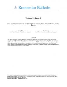
Figure 1: The plots of CUSUM and CUSUM of Squares statistics Apart from that, batteries of diagnostic tests are conducted for the final ARDL model. Specifically, the Ramsey RESET test indicates that the model is correctly specified. The Breusch-Godfrey LM test shows that the residuals are not serially correlated. Furthermore, the ARCH test exhibits no heteroskedasticity in the residuals term. However, the plot of CUSUM of Squares statistics crosses the 5 per cent critical bounds (see Figure 1). This implies that the estimated coefficients are not stable during the period of 1980 to 1998. To affirm the presence of long run equilibrium relationship between savings and investment in Malaysia, a joint significance F-test for H 0 : a= a= 0 is performed. The 2 3 computed F-statistics is 1.984 which is smaller than the 10 per cent upper critical values I(1), indicating that the savings and investment in Malaysia are not cointegrated. This finding may shed some light that capital is mobile internationally over the sample period. However, this result is inconsistent with the finding of Anoruo (2001) and Ang (2007) who found that savings and investment are cointegrated in Malaysia. In view of this conflicting result, we believe that differences in sample period, method and the presence of structural break(s) in the time series data may be the plausible explanations (see Engel, 1996; Cook and Vougas, 2007). Therefore, in the next section, we attempt to investigate the stability of cointegrating relationship between the savings and investment through the rolling windows procedure. 4.3

Rolling windows bounds test results 3.0 2.5 2.0 1.5 1.0 0.5 0.0 84 86 88 90 92 94 96 98 00 02 04 06

Figure 2: The plot of normalized F-statistics for rolling windows bounds test

2245

8


Figure 2 records the normalized F-statistics of bounds test with the rolling windows size of 25. The results of rolling windows ARDL cointegration test show a structural break at 1998. This is corroborating with the breakpoint(s) observed in the ZA and LP unit root tests. A remarkable finding emerges from the rolling windows bounds test approach is that the change of exchange rate regime from floating to fixed owing to the Asian financial crisis has altered the cointegrating relationship between the savings and investment in Malaysia. In particular, the estimation results show that savings and investment are cointegrated from 1960 to 1997; however these variables are not coalescing in the long run from 1998 to 2007. This implies that the degree of international capital mobility is higher after the imposed of fixed exchange rate regime in September 1998. 3 This result is contrary to the finding of Miller (1988) and De Vita and Abbott (2002) as they showed that the degree of capital mobility should be low under the fixed exchange rates regime. However, our finding of high capital mobility under the Ringgit pegged regime is not an unexpected result. This is because the fixed exchange rate regime will provides a less risky environment for investors and the country may be able to attract more influx of foreign funds to finance the domestic investment (see Razin and Rubinstein, 2006). Therefore, the degree of capital mobility is expected to be high under the fixed exchange rate regime. In addition, our finding is also parallel with Kaya-Bahçe and Özmen (2008) who found that the capital mobility is high under the fixed exchange rate regime for Hong Kong, Malaysia and Singapore. In this respect, policy targeting on investment through increasing domestic savings may not effective in Malaysia.

5. CONCLUSIONS The purpose of this study is to revisit the Feldstein and Horioka (1980) puzzle for Malaysia over the sample period of 1960 to 2007. In particular, we are interested to know whether the savings and investment rates are cointegrated. This issue is of interest because it is directly related to the formulation and implementation of appropriate macroeconomic policies to foster economic growth in Malaysia. The findings of this study are summarized accordingly. First, the LP unit root tests with two structural breaks cannot reject the null hypothesis of a unit root for savings and investment rates. This implies that if the savings or investment rates expose to shocks (e.g. oil prices shock in 1973, economic recession in 1985 and Asian financial crisis in 1997), these variables will not return to their long run stable growth path and the effect of the shocks will be permanent. Second, the result of bounds testing approach to cointegration indicates that the variables are not cointegrated with the sample period of 1960 to 2007. This implies that the savings and investment rates will not moving together in the long run. According to the F-H hypothesis, the degree of international capital mobility is rather high in Malaysia. Third, we propose the rolling windows bounds testing approach to cointegration to examine the stability of cointegrating relationship between the savings and investment rates in Malaysia. The findings suggest that the savings and investment rates in Malaysia are not always cointegrated. This may be the reason why the empirical studies in the literature thus far produced mixed results. In addition, our finding is consistent with Bahmani-Oskooee and Bohl (2000) and Bahmani-Oskooee (2001) notions that the presence of cointegration may not 3

Capital control was imposed together with the fixed exchange rate regime in 1998. The capital control is to restrict the flows of short-term investment to reduce vulnerabilities to external shock. However, the flow of long-term investments (i.e. FDI inflows or outflows) remained free as before the capital control (Poon, 2006). Therefore, it does not affect the long-term international capital mobility. 2246

9


implied stability. In particular, we find that the cointegrating relationship vindicate merely from 1960 to 1997, however the variables are not coalescing in the long run after 1998. This implies that the international capital mobility is higher after the Asian financial crisis and the Ringgit pegged regime. This is because the Ringgit pegged regime will provide a less risky business environment for investors and Malaysia may be able to attract more inflow of long term foreign capitals to finance the domestic investment (see Razin and Rubinstein, 2006). Furthermore, the evidence also indicates that the investment in Malaysia is exogenous and thus policies that aim to increase investment through increasing domestic savings are unlikely to be successful.

REFERENCES Anoruo, E. (2001) “Saving-investment connection: Evidence from the ASEAN countries” The American Economist 45, 46-53. Ang, J.B. (2007) “Are saving and investment cointegrated? The case of Malaysia (19652003)” Applied Economics 39, 2167-2174. Athukorala, P. and K. Sen (2002) Saving, Investment, and Growth in India, Oxford University Press: Oxford. Bahmani-Oskooee, M. (2001) “How stable is M2 money demand function in Japan?” Japan and the World Economy 13, 455-461. Bahmani-Oskooee, M. and M. Bohl (2000) “German monetary unification and the stability of the German M3 money demand function” Economics Letters 66, 203-208. Baxter, M. and M.J. Crucini (1993) “Explaining saving-investment correlations” American Economic Review 83, 416-436. Cook, S. and D. Vougas (2007) “Spurious levels relationships” Journal of Interdisciplinary Mathematics 10, 433-439. Crowder, W.J. and C. Phengpis (2007) “A re-examination of international inflation convergence over the modern float” Journal of International Financial Markets, Institutions and Money 17, 125-139. De Vita, G. and A. Abbott (2002) “Are saving and investment cointegrated? An ARDL bounds testing approach” Economics Letters 77, 293-299. Dickey, D.A. and W.A. Fuller, W.A. (1979) “Distributions of the estimators for autoregressive time series with a unit root” Journal of American Statistical Association 74, 427-431. Dickey, D.A. and W.A. Fuller (1981) “Likelihood ratio statistics for autoregressive time series with a unit root” Econometrica 49, 1057-1072. Enders, W. (2004) Applied Econometric Time Series, 2nd Edition, John Wiley & Sons: New York. Engel, C. (1996) “The forward discount anomaly and the risk premium: A survey of recent evidence” Journal of Empirical Finance 3, 123-192. Engle, R.F. and C.W.J. Granger (1987) “Co-integration and error-correction: Representation, estimation and testing” Econometrica 55, 987-1008. Feldstein, M. (1983) “Domestic saving and international capital movements in the long run and the short run” European Economic Review 21, 129-151. Feldstein, M. and C. Horioka (1980) “Domestic saving and international capital flows” Economic Journal 90, 314-329. Granger, C.W.J. and P. Newbold (1974) “Spurious regression in econometrics” Journal of Econometrics 2, 111-120.

2247

10


Gulley, O.D. (1992) “Are saving and investment cointegrated? Another look at the data” Economics Letters 39, 55-58. Hakkio, C.S. and M. Rush (1991) “Cointegration: How short is the long run?” Journal of International Money and Finance 10, 571-581. Kaya-Bahçe, S. and E. Özmen (2008) “Exchange rate regimes, saving glut and the FeldsteinHorioka puzzle: The East Asian experience” Physica A 387, 2561-2564. Kutan, A.M. and S. Zhou (2003) “Has the link between the spot and forward exchange rates broken down? Evidence from rolling cointegration tests” Open Economies Review 14, 369-379. Lee, J. and M.C. Strazicich (2003) “Minimum Lagrange multiplier unit root test with two structural breaks” Review of Economics and Statistics 85, 1082-1089. Lee, J. and M.C. Strazicich (2004) “Minimum LM unit root test with one structural break” Department of Economics, Appalachian State University. Lumsdaine, R.L. and D.H. Papell (1997) “Multiple trend breaks and the unit roots hypothesis” Review of Economics and Statistics 79, 212-218. Mamingi, N. (1997) “Saving-investment correlations and capital mobility: The experience of developing countries” Journal of Policy Modeling 19, 605-626. Miller, S.M. (1988) “Are saving and investment co-integrated?” Economics Letters 27, 3134. Murphy, R.G. (1984) “Capital mobility and the relationship between saving and investment rates in OECD countries” Journal of International Money and Finance 3, 327-342. Narayan, S. and P.K. Narayan (2005) “A empirical analysis of Fiji’s import demand function” Journal of Economic Studies 32, 158-168. Narayan, P.K. and R. Smyth (2006) “Higher education, real income and real investment in China: Evidence from Granger causality tests” Education Economics 14, 107-125. Obstfeld, M. (1986) “Capital mobility in the world economy: Theory and measurement” Carnegie-Rochester Conference Series on Public Policy 24, 55-103. Oscar, B.R. (1998) “The saving-investment correlation revisited: The case of Spain, 19641994” Applied Economics Letters 5, 769-772. Pattichis, C.A. (1999) “Price and income elasticities of disaggregated import demand: Results from UECMs and an application” Applied Economics 31, 1061-1071. Pelagidis, T. and T. Mastroyiannis (2003) “The saving-investment correlation in Greece, 1960-1997: Implications for capital mobility” Journal of Policy Modeling 25, 609616. Perron, P. (1989) “The great crash, the oil price shock and the unit root hypothesis” Econometrica 57, 1361-1401. Pesaran, M.H., Y. Shin, and R.J. Smith (2001) “Bounds testing approaches to the analysis of level relationships” Journal of Applied Econometrics 16, 289-326. Phillips, P.C.B. (1986) “Understanding spurious regression in econometrics” Journal of Econometrics 33, 311-340. Phillips, P.C.B. and P. Perron (1988) “Testing for unit root in time series regression” Biometrika 75, 335-346. Poon, W.C. (2006) The Development of Malaysian Economy, Prentice Hall: Kuala Lumpur. Razin, A. and Y. Rubinstein (2006) “Evaluation of currency regimes: The unique role of sudden stops” Economic Policy 21, 119-152. Solow, R.M. (2001) “Applying growth theory across countries” World Bank Economic Review 15, 283-288. Summer, L.H. (1988) “Tax policy and international competitiveness” in: International Aspect of Fiscal Policies by J. Frenkel, Eds., NBER Conference Report. Chicago University Press, 349-375. 2248

11


Tang, C.F. (2010) “The money-prices nexus for Malaysia: New empirical evidence from the time-varying cointegration and causality tests” Global Economic Review 39, 383-403. Turner, P. (2006) “Response surfaces for an F-test for cointegration” Applied Economics Letters 13, 479-482. Vos, R. (1988) “Saving, investment and foreign capital flows: Have capital markets become more integrated?” Journal of Development Studies 24, 310-334. Zivot, E. and D.W.K. Andrews (1992) “Further evidence of the greater crush, the oil price shock and the unit-root hypothesis” Journal of Business and Economic Statistics 10, 251-270.

2249

12