Vortex dynamics for two-dimensional XY models

Vortex dynamics for two-dimensional XY models Beom Jun Kim, Petter Minnhagen, and Peter Olsson

arXiv:cond-mat/9806231v2 [cond-mat.supr-con] 27 Apr 1999

Department of Theoretical Physics, Ume˚ a University, 901 87 Ume˚ a, Sweden Two-dimensional XY models with resistively shunted junction (RSJ) dynamics and time dependent Ginzburg-Landau (TDGL) dynamics are simulated and it is verified that the vortex response is well described by the Minnhagen phenomenology for both types of dynamics. Evidence is presented supporting that the dynamical critical exponent z in the low-temperature phase is given by the scaling prediction (expressed in terms of the Coulomb gas temperature T CG and the vortex renormalization given by the dielectric constant ˜ ǫ) z = 1/˜ ǫT CG − 2 ≥ 2 both for RSJ and TDGL and that the nonlinear IV exponent a is given by a = z + 1 in the low-temperature phase. The results are discussed and compared with the results of other recent papers and the importance of the boundary conditions is emphasized. PACS numbers: 74.50+r, 74.40+k, 74.25.Fy, 74.76.-w

an intermediate current range whereas aAHNS should be recovered in the true small-current limit.5 This argument rests on the assumption that for any finite current there are free vortices present and furthermore that these free vortices can be described by a conventional dynamics with z = 2.5 In this paper we present extensive simulations of 2D XY models with RSJ as well as TDGL dynamics using an unconventional boundary condition. This enables us to obtain more information on the vortex dynamics for these models. The situation is roughly the following: The MP form of the dynamical response gives a good description of the 2D XY models with TDGL dynamics,7 the Coulomb gas model with Langevin dynamics,10 and experiments on 2D superconductors.7,13,14 In the present paper we show that it also gives a good description of 2D XY models with RSJ dynamics. The dynamical exponent z for the lattice Coulomb gas with Monte Carlo dynamics has from simulations been inferred to have the scaling value z = ascale − 1.11 In the present paper we verify this result for the XY models with both RSJ and TDGL dynamics. This is seemingly in contradiction to the results in Ref. 8 that the 2D XY models with RSJ and TDGL dynamics behave differently and appear to have different z values. The nonlinear IV exponent a has been found to have the scaling value ascale for the Coulomb gas with Langevin dynamics10 and the lattice Coulomb gas with Monte Carlo dynamics.11 However, contradictory results have been found for the XY model with RSJ dynamics, e.g., a = aAHNS in Ref. 9 and a = ascale in Ref. 12. In the present paper we find support for a = ascale for the 2D XY model with RSJ dynamics. The picture emerging from our perspective is a generic vortex response well described by the MP form of the frequency response, the scaling exponent ascale and the corresponding dynamical exponent z = ascale −1. According to our view this generic vortex response describes both Coulomb gas models and 2D XY models and is insensitive to the detailed type of the dynamics be it Coulomb

I. INTRODUCTION

Superconducting films and two-dimensional (2D) Josephson junction arrays as well as 4 He films undergo Kosterlitz-Thouless (KT) type transitions from the superconducting/superfluid to the normal state.1,2 The KT transition is driven by thermally created vortexantivortex pairs which start to unbind at the transition.2 This means that some dominant characteristic features of the physics close to the transition are associated with vortex pair fluctuations. The great current interest in 2D vortex fluctuations stems from the fact that they are also present in high-Tc superconductors, not only in the case of thin films, but also in 3D samples just above the transition.3 It is therefore of interest to understand the properties associated with these thermally created vortices. Whereas there is a fairly good consensus on the static properties associated with vortex pair fluctuations,3 the dynamical aspects are less clear and some features are still controversial. The knowledge of the dynamical properties of vortex fluctuations mainly comes from experiments on superconducting films and 4 He films,2,3 and from various model simulations.3 The theoretical attempts are so far on a rather phenomenological level2,4,5 with few exceptions.6 The more explicit knowledge derives from several kinds of simulations: XY models with time dependent Ginzburg-Landau (TDGL) dynamics,7 XY models with resistively shunted Josephson junction (RSJ) dynamics,8,9 the Coulomb gas model with Langevin dynamics,10 and the lattice Coulomb gas model with Monte Carlo dynamics.11 There exist two phenomenological descriptions: the Ambegaokar-Halperin-Nelson-Siggia (AHNS) description4 and the Minnhagen phenomenology (MP).2 There are, likewise, two distinct proposals for the nonlinear IV exponent a, i.e., aAHNS (Ref. 4) and ascale (Ref. 12) with a corresponding proposal for a critical dynamical exponent z = ascale − 1 (Ref. 12) in the lowtemperature phase. It has also been argued that the nonlinear IV exponent with the value ascale applies to 1

and with this choice the model is the usual 2D XY model or the planar rotor model. This particular interaction would, e.g., arise if each lattice point was a small superconducting island which was Josephson coupled to its nearest neighbors, and the system is called a Josephson junction array (JJA). We will use this choice of the interaction in the present paper. However, from the point of view of vortex fluctuations any U (φ) fulfilling the necessary requirements stipulated above is a valid choice. A possible generalization is    2 φ 2p2 U (φ) = 2 1 − cos , (2) p 2

gas Langevin-, Monte Carlo-, TDGL-, or RSJ-type. The content of the present paper is the following: In Sec. II we describe the XY -type models and the relevant correlation and response functions, as well as the relation to the vortex and Coulomb gas degrees of freedom. We also discuss the validity of linear response and the relation between the complex impedance and the dielectric function of the Coulomb gas. In Sec. III the dynamical equations are described and the boundary condition is introduced and discussed. Sections IV and V contain our simulation results; Sec. IV the equilibrium ones and Sec. V the result when the system is driven by an external current. Finally in Sec. VI we summarize our results and make some final remarks.

where p = 1 corresponds to the usual XY model. The practical point with such a generalization is that the vortex density increases with increasing p.15 Consequently the vortex response is sometimes easier to extract from simulations for a p value larger than 1.7 The Boltzmann factor for a particular configuration is given by e−HXY /T where T is the temperature in units of kB = 1. From this all thermodynamic properties can be obtained. The mapping between the XY model and the Coulomb gas representation is as follows:16 The effective temperature variable for the Coulomb gas charges is given by T CG = T /[2πJhU ′′ i], where T is the temperature for the XY model, h· · ·i denotes a thermal average, and U ′′ = ∂ 2 U/∂φ2 . The supercurrent through a link is given by JU ′ = J∂U/∂φ. The Coulomb gas charge nl , corresponding to an elementary plaquette of the square lattice l, is given by the directed sum (corresponding to a line integral) over the four links hiji making up the plaquette:16

II. XY MODEL

On a phenomenological level, a 2D superconductor/superfluid can be described by an order parameter ψ(r) = |ψ(r)|eiθ(r) , where |ψ(r)|2 is proportional to the superfluid density and ∇θ(r) is proportional to the superfluid velocity.2 The energy associated with the order parameter is the kinetic energy of the Rcurrent and consequently the energy is proportional to d2 r[∇θ(r)]2 /2.2 A positive (negative) vortex centered at a certain point is associated with the topological excitation characterR ized by that the line integral ∇θ(r) · dl of an arbitrary small closed loop around the point is equal to 2π (−2π). There is a precise mapping between the vortices of a 2D superconductor and 2D Coulomb gas charges.2 Since our interest in the present paper is the dynamical effects of the thermal vortex fluctuations, we will describe our results in the language of 2D Coulomb gas charges. The XY -type models in a broad sense are models representing the continuum order parameter ψ(r) = |ψ(r)|eiθ(r) put on a lattice. Let us for convenience choose a square lattice. The discretized version is then ψj = |ψj |eiθj , where the index j denotes the lattice points. Let us simplify further by neglecting the variations of the magnitude of the order parameter and take |ψj | = |ψ| to be a constant. The discretized version of the energy then takes the form X U (φij = θi − θj ), (1) HXY = J

nl ≡

T CG X ′ U. T hiji∈l

ˆ t) is a key quantity and is The correlation function G(k, defined by ˆ t) ≡ 1 hFˆ (k, t)Fˆ (−k, 0)i, G(k, Ω where Fˆ (k, t) is the 1D Fourier transform

hiji

Fˆ (k, t) =

where J ∝ |ψ|2 is termed the XY coupling constant and the sum is over nearest-neighbor pairs. The lattice constant is taken to be unity so that φij = θi −θj corresponds to ∇θ (in the direction from j to i). The function U (φ) has to be equal to φ2 /2 for small φ in order to yield the correct continuum limit and in addition U (φ) has to be a periodic function of 2π since the phase angle θi for each lattice point is only defined upto a multiple of 2π. A possible choice for U (φ) is then

X

Fm (t)eikm ,

m

m labels the rows of the lattice, and finally Fm (t) = J

X

U ′ [φij (t)],

hiji∈m

where the summation is over all the links making up the row m. The Fourier transformation of the charge density ˆ t) by correlation function gˆ(k, t) is related to G(k,

U (φ) = 1 − cos φ 2

ˆ t) = G(k,



T T CG

2

gˆ(k, t) . k2

KT transition whereas it can only be approximately correct above because of the presence of free vortices which always dominates the response for small enough frequencies and gives a Drude-like response in this limit.7 In the present paper we focus on the low-temperature phase. In this case the leading small ω behavior of Eqs. (8) and (9) reflects a 1/t decay for large t of the function ˆ = 0, t).12 One may also observe that Eq. (9) leads to G(k a logarithmic divergence of the real part of the conductivity: σ(ω) ∼ −ωIm[1/ˆ ǫ(k = 0, ω)] ∼ − ln ω for small ω, which is compatible with standard scaling argument by Fisher and Fisher, Fisher, and Huse in Ref. 19.20 −[(1/˜ ǫT CG )−2] The two features and R 2 G(r, t = 0) ∝ r ˆ G(k = 0, t) = d rG(r, t) ∝ 1/t can be turned into an argument for the dynamical critical index z in the following way:12 We assume that G(r, t) must be of the form

(3)

Linear-response theory then links gˆ(k, t) with the dielectric response function 1/ˆ ǫ(k, ω) by7   Z 1 2πωT CG ∞ 1 ˆ t), Re + = dt sin ωt G(k, ǫˆ(k, ω) ǫˆ(k, 0) T2 0 (4)

Im



 Z 1 2πωT CG ∞ ˆ t), =− dt cos ωt G(k, ǫˆ(k, ω) T2 0

(5)

where 2πT CG ˆ 1 G(k, 0). =1− ǫˆ(k, 0) T2

(6)

G(r, t) ∝ λα f (r/λ, t/τ, a/r, τa /t),

ˆ t) will be of particular The quantities 1/ˆ ǫ(0, ω) and G(0, interest in the present investigation. The thermodynamic KT transition is characterized by lim

k→0

where λ is the correlation length or screening length which diverges in the low-temperature phase, τ is the corresponding diverging relaxation time so that

1 1 = >0 ǫˆ(k, 0) ǫ˜

τ ∝ λz , where z is the dynamical exponent. In addition we have a short distance scale a, i.e., the lattice constant or the size of a Coulomb gas particle and a nondiverging characteristic time scale τa , i.e., τa ∝ l2 /D where D is a vortex or Coulomb particle diffusion constant and√l is some nondiverging length scale like l = a or l = 1/ n where n is the density of Coulomb gas particles. Let us choose t = 0 and r = λ so that

below the transition and lim

k→0

1 =0 ǫˆ(k, 0)

above. Precisely at the transition limk→0 1/ˆ ǫ(k, 0)T CG jumps from the universal value 1/˜ ǫT CG = 4 to zero.17,18 The equal-time correlations fall off like power laws with distance below the transition and exponentially above.2 For example, the correlation function G(r, t = 0) falls off like G(r, 0) ∝ r

−(1/˜ ǫT CG −2)

G(r, 0) ∝ rα f (1, 0, a/r, ∞) and make the ad hoc scaling assumption that

(7)

lim f (1, 0, a/r, ∞) = f (1, 0, 0, ∞) = const,

r→∞

below the transition temperature. The fact that the correlations decay algebraically with distance reflects that the whole low-temperature phase is quasicritical. As explained in the previous section one motivation for the present paper is the question of the generality of the MP form for the dynamical response, which is given by2   1 1 ω 1 Re = , (8) − ǫˆ(k = 0, ω) ǫˆ(0, 0) ǫ˜ ω + ω0  2 ωω0 ln ω/ω0 1 =− . Im ǫˆ(k = 0, ω) ǫ˜π ω 2 − ω02 

where const6= 0 and 6= ±∞. This requires α = CG −1/˜ ǫT CG + 2 since G(r, 0) ∝ r−[(1/˜ǫT )−2] . We then also have that Z Z CG d2 rG(r, t) = λ−(1/˜ǫT )+2 d2 rf (r/λ, t/τ, a/r, τa /t). 1

Now we choose λ = t z so that Z Z CG d2 rG(r, t) = t[−1/˜ǫT +2]/z d2 rf (r/t1/z , 1, a/r, τa /t) and assume that

(9)

lim f (r/t1/z , 1, a/r, τa /t) = f (0, 1, a/r, 0) = f˜(a/r),

t→∞

The characteristic frequency ω0 vanishes as the KT transition is approached from above and below.7 The idea behind the MP form is that it describes the response due to the bound pairs. Consequently, it is expected to have the correct leading small-frequency behavior below the

where f˜(x) is a well-behaved function so that Z Z CG d2 rG(r, t) ∝ t[−(1/˜ǫT )+2]/z d2 rf˜(a/r) 3

for large t. This is consistent with provided

R

˙ t) + JU ′ [∇x θ(r, t)] ix (r, t) = −∇x θ(r,

d2 rG(r, t) ∝ 1/t

1 − 2. z= ǫ˜T CG

in some convenient unit system. The voltage in the RSJ model is proportional to the normal current so we can define the response function corresponding to the complex impedance as Z(r − r′ , t − t′ ) = P˙ (r − r′ , t − t′ ), where ∂h∇x θ(r, t)i ′ ′ . (14) P (r − r , t − t ) = − ∂ix (r′ , t′ ) ix =0

(10)

The dynamical exponent z given by Eq. (10) has been inferred through simulations of the lattice Coulomb gas with Monte Carlo dynamics.11 In the present paper we conclude that the same is true for the XY models both with RSJ and TDGL dynamics. It has been argued by Dorsey,21 using scaling analysis, that for a 2D superconductor the exponent a in the nonlinear IV characteristics V ∝ I a has the value a = z + 1 precisely at the KT transition. It has further been suggested by Minnhagen12 that since the whole low-temperature phase is quasicritical the same relation should apply throughout the low-temperature phase. This together with Eq. (10) leads to the prediction a = ascale = z + 1 =

1 − 1. ǫ˜T CG

It is shown in the appendix that the Fourier transform of P is given by  −1 ρ0 ˆ P (k, ω) = iω + , (15) ǫˆ(k, ω)

where ρ0 = JhU ′′ i so that −1  ˆ ω) = 1 + 1 ρ0 . Z(k, iω ǫˆ(k, ω)

(11)

lim lim

ω→0 k→0

1 =∞ ǫˆ(k, ω)

so that the static response to a uniform static current below the KT transition is nonlinear. However, for any finite frequency the response is linear to the lowest order. One also notes that in the limit of high frequency 1/iωˆ ǫ(k, ω) vanishes and Zˆ in Eq. (16) reduces to Z(∞) = 1, which means that the response in this limit is given by the resistive shunt in the RSJ model. For smaller frequencies the response is given by the vortex fluctuation Z(ω) ∝ iωˆ ǫ(0, ω)/ρ0 as already stated in Eq. (12).

E(ω) = Z(ω)j(ω), where E(ω) is the frequency dependent electric field and j(ω) is the current density. Or equivalently for a quadratic sample V (ω) = Z(ω)I(ω), where V is the voltage across the superconductor in some direction and I is the total current in the same direction. The linearresponse function Z −1 (ω) is related to the Coulomb gas linear-response function 1/ˆ ǫ(k = 0, ω) by ρ0 , iωˆ ǫ(k = 0, ω)

(16)

This means that the response to a uniform time varyˆ ω). Below the KT ing current is given by Z(ω) = Z(0, transition we have

The nonlinear IV exponent a = ascale in Eq. (11) has been inferred through simulations for the Coulomb gas model with Langevin dynamics10 and the lattice Coulomb gas model with Monte Carlo dynamics.11 The response to an imposed current is for a 2D superconductor given by the complex impedance Z(ω):2,22

Z −1 (ω) ∝

(13)

III. DYNAMICAL EQUATIONS AND BOUNDARY CONDITIONS

(12)

where ρ0 is the density of superconducting electrons which for an XY model is given by JhU ′′ i. This means that the effect on the vortex fluctuations of an imposed current is given by 1/ˆ ǫ(k = 0, ω). For small ω this is the dominant contribution. It is instructive to consider the linear response to an imposed current directly in the the case of the XY model with RSJ dynamics. Let us consider a quadratic lattice and let hijix be a link at position r parallel to the x axis and denote the difference in phase angle by φij = ∇x θ(r); when the coupling to the electromagnetic field is included φij denotes the gauge invariant phase difference. The supercurrent through the link at time t is JU ′ [∇x θ(r, t)] ˙ t) and the normal current is proportional to −∇x θ(r, where the dot denotes the time derivative. Thus the total current ix (r, t) through the link is

Simulations by necessity involve lattices with a finite linear dimension L from which the results for the thermodynamic limit L → ∞ have to be extracted. This means that in practice the choice of boundary condition is essential.23 The most commonly used boundary condition in order to extract the thermodynamic limit for the XY models is periodic boundary conditions (PBC) imposed on the phase angles θi . However, as discussed in Ref. 16, the PBC for the phase angles leads to a nonperiodic boundary condition for the vortex interaction. The boundary condition for the phase angles which corresponds to a periodic vortex interaction is instead the fluctuating twist boundary condition (FTBC).16 The dynamics we are investigating in the present paper are linked to the vortex fluctuations and consequently the natural boundary condition is PBC for the vortices. This 4

is the commonly used boundary condition for simulations of the lattice Coulomb gas with Monte Carlo dynamics11 and the continuum Coulomb gas with Langevin dynamics.10 Thus the important point in the present context is that PBC for the vortices means FTBC for the phase angles. The FTBC for the phase angles has so far been used in connection with Monte Carlo simulations.16 In the present paper we extend the use of these boundary conditions to XY models with RSJ and TDGL dynamics.24 Of course the boundary condition should not matter in the limit L → ∞. However, we in the present paper find that by using FTBC for the phase angles we are able to extract more information from our finite L simulations. In this section, we briefly review the dynamical equations of motion for RSJ and TDGL in the case of PBC for the phase angles. Then we construct the equations of motion for FTBC starting from total current conservation and the condition that the equations of motion should lead to the correct equilibrium distribution. We focus on the ordinary XY model, which corresponds to p = 1 case in the previous section, but the extension to a general p is straightforward. We begin with an L×L array of the resistively shunted junctions with PBC in both directions. In the RSJ dynamics of 2D XY model the net current from site i to site j is written as the sum of the supercurrent, the normal resistive current, and the thermal noise current: iij = ic sin(φij = θi − θj ) +

¯h

where Γ is a dimensionless constant Pwhich determines the time scale of relaxation, H ≡ −J hiji cos(θi − θj ) is the Hamiltonian of the usual XY model, and θi is periodic in both directions. The thermal noise term Γi (t) is assumed to satisfy hΓi (t)i = 0 and hΓi (t)Γj (0)i = 2¯ hΓkB T δij δ(t). After rescaling the time and the temperature in units of ¯h/ΓJ and J/kB , respectively, the equations of motion for TDGL dynamics are written as θ˙i = −

X j

Gij

X′ k

sin(θi − θj ) + ηi ,

(19)

(20)

In numerical simulations for PBC, we use Eqs. (17) and (19) for RSJ and TDGL dynamics, respectively, with the corresponding thermal noises satisfying Eqs. (18) and (20). Next we consider the fluctuating twist boundary condition FTBC. In this case a variable ∆ ≡ (∆x , ∆y ) is introduced and the phase difference φij on the bond (i, j) is changed into16 θi − θj − rij · ∆,

(21)

where rij ≡ rj − ri is a unit vector from site i to j, and the phase angles are periodic: θi = θi+Lˆx = θi+Lˆy . In the study of equilibrium behaviors for FTBC using MC simulations, it is sufficient to know the Hamiltonian of the system16 X cos(θi − θj − rij · ∆). (22) H = −J hiji

In dynamical simulations, on the other hand, we must also have equations of motion for the new variables ∆x and ∆y in addition to the equations of motion for phase variables θi . The physical situation we have in mind is a sample where no current passes through the boundary. For the RSJ model, which has local current conservation, Rthis 2 implies the total current conservation condition dr i(r, t) = 0, where i(r, t) = [ix (r, t), iy (r, t)] is the total current density at point r and the integral is over the whole sample. This condition can also be expressed as Vx ic X (23) sin(θi − θj − ∆x ) − η∆x =− r L

(17)

where the primed summation is over four nearest neighbors of j, Gij is the lattice Green function on the square lattice with PBC, ηjk is the dimensionless thermal noise current defined by ηjk ≡ Γjk /ic , and the unit of time is h/2eric . The thermal noise current satisfies hηij (t)i = 0 ¯ and hηij (t)ηkl (0)i = 2T (δik δjl − δil δjk )δ(t),

j

hηi (t)ηj (0)i = 2T δij δ(t).

Vij + Γij , r

[sin(θj − θk ) + ηjk ],

X′

where the thermal noise term ηi ≡ Γi /ΓJ satisfies hηi (t)i = 0 and

where ic ≡ 2eJ/¯ h is the critical current of the single junction, Vij is the potential difference across the junction, r is the shunt resistance, and the phase angles θi are periodic in both directions (θi = θi+Lˆx = θi+Lˆy ). The thermal noise current Γij at temperature T is required to satisfy hΓij (t)i = 0 and hΓij (t)Γkl (0)i = (2kB T /r)δ(t)(δik δjl − δil δjk ). The current-conservation law at each site, together with the Josephson relation d(θi − θj )/dt = 2eVij /¯ h, allows us to write the equations of motion in the form θ˙i = −

∂H dθi (t) + Γi (t), = −Γ dt ∂θi

(18)

hijix

(and the similar P equation for the y direction), where the summation hijix is over all nearest-neighboring pairs in x direction, Vx is the voltage drop over the sample,

where T is in units of J/kB . In the TDGL dynamics with PBC, on the other hand, the equations of motion are given by25 5

W = e−βH with the Hamiltonian given by Eq. (22) provided

and η∆x denotes the thermal noise current. This follows because the left-hand side is recognized as the normal current whereas the right-hand side is the negative of the sum of the supercurrent and the noise current. As discussed in connection with Eq. (13) the voltage is by ˙ t). For the the Josephson relation proportional to ∇θ(r, voltage across the sample this means that [see Eq. (21)] ˙ x = − 2e Vx , ∆ hL ¯

βσ 2 = βT = 1, 2 2 1 βσ∆ = 2, 2 L

˙ = −Γ∆ ∂H + η∆ ∆ ∂∆

(26)

hijiy

where we have again written t in units of h ¯ /2eric . Next a noise correlation consistent with the equilibrium condition has to be found. To this end we make the ansatz of a standard white-noise correlation hη∆x (t)η∆x (0)i = 2 δ(t) and determine the appropriate hη∆y (t)η∆y (0)i = σ∆ 2 σ∆ in the following way: The equations of motion for the phase variables in FTBC are written as X X′ j

Gij ηjk ,

(27)

sin(θj − θk − ∆jk )

(28)

θ˙i = −

X j

Gij

X′ k

X′ j

sin(θi − θj − rij · ∆) + ηi ,

(32)

where we have used the dimensionless time t by introducing the time unit of h ¯ /ΓJ as in Eq. (19). Just as for the RSJ case one finds that Γ∆ = 1/L2 and that the noise correlation hη∆x (t)η∆x (0)i = hη∆y (t)η∆y (0)i = (2T /L2 )δ(t) leads to the correct equilibrium. To some extent the TDGL dynamics may be viewed as a simplified version of the RSJ dynamics where the total current conservation is kept but the local current conservation is relaxed. Thus from this point of view it is perhaps not surprising that the two models (as we will see) have the same generic vortex dynamics. The twist variable ∆ plays an important role in our analysis of the vortex dynamics and there exists a rather direct connection between the twist and the vortices: The electric field E(t) due to the vortex current density jv is perpendicular and is, as a consequence of the Josephson relation, given by11

k

with hi ≡ −

(31)

with Γ∆ = 1/L2 and hη∆x (t)η∆x (0)i = hη∆y (t)η∆y (0)i = (2T /L2 )δ(t). In the TDGL model the total current conservation condition can still be imposed whereas the local current conservation condition is relaxed. Thus Eqs. (25) and (26) remain unaltered whereas the equations for the phase angles are simplified to [compare Eqs. (19) and (21)]

hijix

θ˙i = hi −

(30)

2 and consequently σ∆ = 2T /L2. The equation of motion for the twist variables are hence of the Langevin form

(24)

because the phase angles are by construction subject to periodic boundary conditions. Thus from Eqs. (23) and (24), we obtain the equations of motion for the twist variables: 1 X d∆x = 2 (25) sin(θi − θj − ∆x ) + η∆x , dt L d∆y 1 X = 2 sin(θi − θj − ∆y ) + η∆y , dt L

(29)

and hηij (t)ηkl (0)i = σ 2 (δik δjl − δil δjk )δ(t), where σ 2 = 2T [see Eq. (18)]. From the full equations of motion for RSJ model in FTBC [Eqs. (25) – (27)], we arrive at the Fokker-Planck equation:26 X ∂ ∂W ∂ ∂ (hi W ) − (hx W ) − (hy W ) =− ∂t ∂θi ∂∆x ∂∆y i   ∂2W 1 2 ∂2W ∂2W 1 2X Gij , + σ∆ + + σ 2 ∂θi ∂θj 2 ∂∆2x ∂∆2y i,j

E=

h hjv (t)i. 2e

where W = W ({θi }, ∆x , ∆y ; t) is the probability distribution function and 1 X hx ≡ 2 sin(θi − θj − ∆x ), L

˙ is discussed in The connection between hjv (t)i and ∆ Ref. 16; when a vortex moves across the sample then the twist variable changes by 2π/L. In other words, if the time t0 is associated with the movement of a vortex across ˙ = 2π/Lt0 = 2πhvi/L2 where the sample, then we get ∆ |hvi| = L/t0 is the vortex velocity. If there are Nv moving ˙ = 2π(Nv /L2 )hvi = 2πhjv i, vortices, then we obtain ∆ which leads to the relation given by Eq. (24):

and the similar equation for hy . The stationary solution, which satisfies ∂W/∂t = 0, is of the correct form

˙ x = − 2e Vx , ∆ ¯hL

hijix

6

introduced by the discretization. In order to get a handle of the choice for ∆t we use the following identity: Let us introduce a local variable ak on one particular site k. The Hamiltonian of the system is then X U (θi − θj + ai − aj ) H=

where Vx is the voltage drop across the sample in x direction (we obtain the similar equation for ∆y ). So far we have considered the situation when the total current in the sample is zero, which corresponds to no current passing over the boundary. Let us now consider the case when the total current is a constant dc current Id in the x direction. By following the steps from Eq. (23) to Eqs. (25) and (26) one obtains the modified equations of motion for the twist variable ∆ 1 X d∆x = 2 sin(θi − θj − ∆x ) + η∆x − id dt L

hiji

with ai 6= 0 for i = k and ai = 0 otherwise, and the partition function is given by Z Y dθi exp(−βH) Z=

(33)

hijix

d∆y 1 X = 2 sin(θi − θj − ∆y ) + η∆y dt L

i

(34)

hijiy

with the inverse temperature β ≡ 1/T . After a simple change of variable θi + ai → θi , we find that Z does in fact not depend on ak and thus

with id = Id /L in units of ic . The voltage drop in the x direction [see Eq. (24)] is given by ˙x Vx = −L∆

∂ 2 ln Z = 0, ∂a2k

(35)

with Vx in units of ric for RSJ and in units of ΓJ/2e for TDGL, respectively. Thus the equations of motion in the presence of an externally imposed dc current Id in the x direction are given by Eqs. (27), (33), and (34) for RSJ and by Eqs. (32), (33), and (34) for TDGL. An alternative and commonly used method in numerical simulations of the current-driven XY model is to impose uniform currents through the boundary in one direction. This requires an open boundary condition for the phase angles in the direction of the applied current and the periodic boundary condition can only be kept in the perpendicular direction.27 This means that an open boundary is explicitly introduced. One advantage with the present method is that the periodic boundary conditions on the phase angles are kept and no explicit boundary is introduced. In the following two sections we present the results obtained from the dynamical equations described in the present section both for the PBC and the FTBC.

from which we conclude that 2 + * X′ 1  U ′ (θk − θj ) , 4hU ′′ i = T j and thus

T = T˜

(36)

provided we have defined T˜ by the local correlations h i2  P ′ ′ U (θ − θ ) k j j T˜ ≡ , (37) 4hU ′′ i where the summation is over four nearest neighbors (denoted by j) of site k. The point is now that for a finite ∆t one finds that T˜ > T . In the present simulations we use the time step ∆t = 0.01 for TDGL and ∆t = 0.05 for RSJ. These choices make T˜ differ from T by less than 3%. The fact that T˜ > T for a finite time step suggests that the effect of the finite time step to some extent is equivalent to an increased temperature. We have tried to take this into account when analyzing quantities related to 1/ˆ ǫ by noting that for FTBC one has 1/ˆ ǫ(0, 0) = 0,16 which means that [compare Eq. (6)]

IV. SIMULATION RESULTS

In this section, we present simulation results for the TDGL and RSJ dynamics with periodic boundary conditions PBC and the fluctuating twist boundary conditions FTBC. For PBC, we use Eqs. (17) and (18) in the RSJ case and in the TDGL case Eqs. (19) and (20). For FTBC, we use Eqs. (25) – (27) for RSJ, and Eqs. (25), (26), and (32) for TDGL. We integrate the equations of motion by discretizing time into small steps ∆t. At each step the appropriate random noise, generated from a uniform distribution, is introduced with hηij (t)2 i = 2T /∆t for RSJ and hηi (t)2 i = 2T /∆t for TDGL [see Eqs. (18) and (20)]. We want to integrate to as long times as possible.28 On the other hand the larger ∆t we choose the larger is the error

T =

ˆ 0) G(0, . hU ′′ i

Thus we can estimate an effective temperature by T eff = ˆ 0)/hU ′′ i. For example, for T = 0.80 and the time G(0, step ∆t = 0.05 we for RSJ get T eff ≈ 0.82 whereas we for TDGL and the time step ∆t = 0.01 get T eff ≈ 0.803. 7

A. Dynamical response functions with periodic boundary conditions

ˆ MP ≈ G

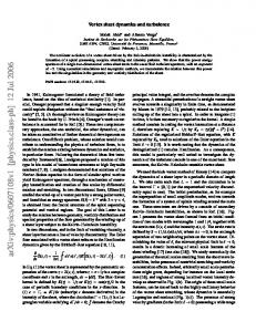
We will first consider the vortex dynamics as reflected in the complex dielectric function given by Eqs. (4) and (5). It has so far been established that the MP form Eqs. (8) and (9) gives a good representation of the experimental data,13 as well as the simulation data for the TDGL dynamics of the XY model on a square lattice with p = 2 and on the triangular lattice with p = 1,7 and the 2D Coulomb gas model.10 In the present investigation we find that the same is true for the XY model with RSJ dynamics. This is illustrated in Fig. 1 which shows the real and imaginary parts of 1/ˆ ǫ(k = 0, ω) − 1/ˆ ǫ(0, 0) with RSJ dynamics for T = 0.85. The full line in the figure has been obtained from a least-square fit to the MP form of the real part in Eq. (8) with two free parameters (˜ ǫ and ω0 ), and the broken line has been obtained by using the same values of the parameters in Eq. (9) (the frequency range in Fig. 1 corresponds to 0.08 < ω/ω0 < 4.7). The MP form has the characteristic feature that the ratio is |Im[1/ˆ ǫ(0, ω)]|/Re[1/ˆ ǫ(0, ω) − 1/ˆ ǫ(0, 0)] = 2/π at the frequency where the imaginary part has its maximum. One sees directly in Fig. 1 (i.e., without any curve fitting) that the dotted vertical line is close to this maximum and it is hence easy to verify that the ratio is indeed close to 2/π. In short, our present simulations of the complex dielectric function confirm that the RSJ dynamics is well described by the MP form at temperatures below as well as somewhat above the critical temperature in agreement with what was found earlier for the TDGL dynamics in Ref. 7.29 As pointed out in connection with Eqs. (8) and (9), the leading small ω dependence of the MP form   1 1 ∝ω − Re ǫˆ(0, ω) ǫˆ(0, 0)

ˆ MMP ≡ G ˆ MP exp(−t/τG ). G

 1 Im ∝ ω ln ω ǫˆ(0, ω) ˆ = 0, t) ∝ 1/t for large t. More precisely, reflects that G(k since   Z ∞ 2 1 1 sin ωt ˆ t) = T dω, G(0, Re − π 2 T CG 0 ω ǫˆ(0, ω) ǫˆ(0, 0) we find for the MP form T2

(39)

ˆ t)] as a function of time for the Figure 2 shows ln[tG(0, system sizes L = 6, 8, 10, 12, 16, and 64 in case of (a) RSJ and (b) TDGL dynamics at T = 0.85. The full drawn curves are least-square fits to Eq. (39). As is apparent ˆ approaches a constant for large lattice from Fig. 2, tG ˆ indeed goes as 1/t for large t both sizes verifying that G for RSJ and TDGL dynamics. The fits to the MMP form (full drawn curves in Fig. 2) ˆ t) goes as −t/τG for large t. In Fig. 3 show that ln tG(0, we have plotted τG [determined by the fit to Eq. (39)] as a function of lattice size L in a log-log scale. From finite-size scaling we expect that in the low-temperature phase τG diverges as τG ∝ Lz for large L where z is the dynamical critical exponent. This behavior corresponds to straight lines in Fig. 3 and the full straight lines in the figure suggest that the asymptotic scaling is reached already for relatively small L. Assuming that this is the case, we find from the slopes of the lines that for T = 0.85 z ≈ 1.6 in case of RSJ and z ≈ 2 for TDGL. Thus the z values in case of PBC are different for the RSJ and the TDGL dynamics. This difference between RSJ and TDGL in case of periodic boundary conditions was also found by Tiesinga et al. in Ref. 8, where in the temperature interval T ∈ [1.1, 1.3] z ≈ 2 for TDGL and z ≈ 0.9 for RSJ; the authors concluded that the TDGL somewhat unexpectedly describes the experiments on Josephson junction arrays by Shaw et al.30 better than the RSJ model. The conclusion we arrive at is different since we find that for FTBC the equivalence between RSJ and TDGL is restored. The apparent difference in case of PBC appears to be a boundary effect.31 We believe that the physical situation in Ref. 30 and most other common experimental situations are in fact better described by the FTBC. Of course, for large enough system sizes, intensive physical quantities do not depend on the explicit choice of boundary condition. But the point here is that, because the relaxation of the zero-k mode is described by a relaxation time τG which diverges for infinite



π 2 ǫ˜T CG

1 . ω0 t

This 1/t tail in the vortex correlations has been verified in Ref. 12 for TDGL dynamics and in Ref. 10 for the Coulomb gas model. We will here verify the same result for the RSJ dynamics. By necessity, the finite lattice sizes used in the simulations introduce a finite relaxation time τG at large t for the zero-k mode. By studying the lattice size deˆ t) we have found that this finite size pendence of G(0, induced relaxation changes the large-t decay from 1/t to ˆ t) for (1/t) exp(−t/τG ). In fact we have found that G(0, finite lattices to a good approximation is of a modifiedMP form (MMP):

and

ˆ MP (0, t) = G

T2 π 2 ǫ˜T CG

[Ci(ω0 t) sin ω0 t − si(ω0 t) cos ω0 t] , (38)

where the cosine and the sine integralsR are defined by R∞ ∞ Ci(x) ≡ − x dt cos t/t and si(x) ≡ − x dt sin t/t, respectively. In the limit of ω0 t → ∞, Eq. (38) reduces to 8

systems, the exponent z, which describes how this divergence is approached, appears to be sensitive to the choice of boundary condition.31 We also note that for T = 0.90 we find z ≈ 1.6 in case of RSJ with PBC. This suggests that z for PBC approaches a value less than 2 as the KT transition is approached from below, although the numerical accuracy may be insufficient to make a firm conclusion.

FTBC the phase difference over the sample in one direction (let us choose the x direction) is given by ∆φ = L∆x . It follows that R can be expressed as R=

L2 1 h[∆x (Θ) − ∆x (0)]2 i, 2T Θ

(41)

where T is in units of J/kB , ∆x (t) is the twist variable in the x direction at time t, and R is in units of the shunt resistance r of a single Josephson junction for the RSJ model and ΓJ/2eic for TDGL model, respectively. Since Eqs. (40) and (41) are identical in the limit of large Θ, i.e., for Θ ≫ τ ,33 we for practical reasons use Eq. (41) in the present simulations (we have used Θ = 16000 and Θ ≫ τ ). Figure 7(a) shows the results for the XY model with RSJ dynamics for T =0.90, 0.85, and 0.80. The data are plotted as log R against log L and to good approximation fall on a straight line, whose slope gives an estimate of the critical exponent z, and we obtain z =2.0, 2.7, and 3.3, respectively. Figure 7(b) shows the same features for the XY model with TDGL dynamics at the same three temperatures T =0.90, 0.85, and 0.80 and the estimated values of z ≈ 2.1, 2.8, and 3.3 are close to the ones obtained for the RSJ dynamics. Thus for the FTBC we find the same z below the KT transition for RSJ and TDGL dynamics, which is in contrast to the PBC case where we found different values of z for each dynamics (compare the discussion of Fig. 3 in Sec. IV). Furthermore for FTBC we find that z apparently approaches 2 when the KT transition is approached from below (T = 0.90 is very close to the KT transition temperature) for both dynamics; this did not seem to be true for the RSJ dynamics with PBC (z ≈ 1.6 at T = 0.90). Our conclusion is that the dynamical critical exponent z is a boundary sensitive quantity. We also note that the FTBC is adequate for describing an open system with voltage fluctuation across the system and that consequently the z values obtained for this case describe the most usual physical situation. It is in fact possible to estimate the characteristic time τ very directly since the variable ∆x changes by the amount 2π/L when a vortex moves across the system in the y direction, as discussed in Sec. III. Every such event consequently is signaled by a 2π step in the time series of the variable L∆x . Figure 8 illustrates this for the RSJ dynamics at T = 0.85 for various system sizes. As seen in the figure the 2π jumps are very well observable. The characteristic time scale τ of these 2π jumps is easily estimated as the average time between the jumps and we expect that τ ∼ Lz with the same dynamical critical exponent z as in R ∼ L−z . Figure 9(a) shows τ plotted against the system size L in a log-log plot for the RSJ dynamics for three different temperatures (in practice we use a coarse graining of 100 time units in our estimate of the average time between the 2π jumps). The full drawn straight lines in Fig. 9(a) have the slopes given by the z values determined previously from the calculation of R [see Fig. 7(a)]. As seen the two ways of determining z

B. Dynamics for the fluctuating twist boundary conditions

In case of FTBC the static dielectric function function 1/ˆ ǫ(k, 0) is identically zero for k = 0, whereas limk→0 1/ˆ ǫ(k, 0) 6= 0 below the KT transition.16 In Ref. 10 it was shown that for the Coulomb gas model with Langevin dynamics the function 1/ˆ ǫ(k, ω) for small k is to good approximation given by the MP form. Since, as explained above in Sec. III, PBC for the vortices (as in Ref. 10) corresponds to FTBC for the XY model we also expect to find the MP form for small k in the present case. This is illustrated in Fig. 4 which shows the real and imaginary parts of 1/ˆ ǫ(k, ω) for k = (0, 2π/L) with L = 64 for the XY model with RSJ dynamics. The full drawn and broken curves represent the MP form just as in Fig. 1 and the dotted line shows that the peak ratio is close to 2/π. Figure 5 demonstrates that the imaginary part depends very little on the k value whereas the real part increases with decreasing k for fixed frequency. This behavior has also been found for the Coulomb gas model with Langevin dynamics (compare Figs. 11 and 12 in Ref. 10). Figure 6 shows how the relaxation time τG of ˆ t) depends on k: G ˆ ∝ (e−t/τG )/t for large t and τG G(k, diverges as k is decreased. In Ref. 10 it was found that τG ∝ k −2 for the Coulomb gas model with Langevin dynamics. Our present convergence is not good enough for establishing this result, but Fig. 6(b) suggests that such a behavior is also consistent with the present simulations of the XY model with RSJ dynamics. Next we turn to the diverging relaxation time τ and the dynamical critical exponent z for the case of FTBC. We will use the fact that in the low-temperature phase the resistance R of a finite system is proportional to 1/τ .32 This follows because of the Nyquist formula:33 Z ∞ 1 dthV (t)V (0)i (40) R= 2kB T −∞ which relates the resistance to the voltage fluctuations over the sample and the fact that V ∝ (d/dt)∆φ where ∆φ is the phase difference over the sample. Since ∆φ is dimensionless it follows that R scales like 1/τ where τ is the relevant characteristic time.32 In the low-temperature phase R vanishes in the limit of large system sizes since τ diverges. Consequently the finite-size scaling R ∝ 1/τ ∝ L−z defines the value of the dynamical critical exponent z in the low-temperature phase. For the XY model with 9

agree very well. Figures 7(b) and 9(b) illustrate the same agreement in case of TDGL dynamics. Let us now consider what happens when a finite current is applied across the system. The scaling argument by Dorsey21 makes use of the fact that the current density J introduces a new length scale 1/J .19 This new length scale replaces the finite size L in the leading L dependence of R, so that34 V = R(J −1 )I ∝

V. NONLINEAR IV CHARACTERISTICS

In order to obtain the IV characteristics for the 2D XY model with RSJ dynamics we use FTBC and Eqs. (33) – (35). Figure 11 shows the data obtained from lattice sizes L = 4 to 64, where v = V /L is plotted against id = Id /L in a log-log plot. As seen from the figure the data are size dependent but for L = 64 the data appear to be reasonably size converged except for the smallest currents. The data in the figure are for T = 0.80 and the straight line is a least-square fit to the L = 64 data in the current interval 0.03 ≤ id ≤ 0.15 and gives a ≈ 4.7, which is in reasonable agreement with ascale = 1/˜ ǫT CG −1 ≈ 4.5. In the following we will investigate the sensitivity of this apparent agreement to finite size, finite current, and boundary conditions. One finite current effect is that the exponent a refers to a constant Coulomb gas temperature T CG = T /[2πJhU ′′ i]. Since a finite current changes the value of hU ′′ i,12 fixed temperature (T = const) is not entirely equivalent to fixed Coulomb gas temperature (T CG = const). In order to convert the data to fixed Coulomb gas temperature we have calculated v and T CG for T = 0.79 and 0.80 for fixed external currents, and then by interpolation estimated the voltage value corresponding to a fixed T CG . The resulting data for a fixed Coulomb gas temperature (T CG ≈ 0.17) are shown in the inset of Fig. 11. The broken line in the inset is a fit to the data and gives a ≈ 4.5. Thus this correction leads to a somewhat smaller value of a. All previous estimates for the nonlinear IV exponent for the RSJ model have been obtained for L = 64 or smaller sizes.9,12,27 The next question we address is how much the possible remaining size effects could alter the results inferred for L = 64. Figure 12 shows voltage v versus the system size L at the external current id = 0.1 and T = 0.8 for three different cases. The open squares at the top correspond to the usual uniform current injection method used in Ref. 27. The filled circles correspond to our FTBC boundary condition and finally the open triangles at the bottom correspond to the busbar boundary condition used in Ref. 9.36 It is clear from the figure that L = ∞ result cannot be estimated by the L = 64 for id = 0.1. For smaller id the situation quickly gets even worse. Thus this unexpected strong size dependency clearly makes all earlier results obtained for a from IV simulations somewhat questionable.9,12,27 As seen in Fig. 12 the uniform current injection appears to approach the L = ∞ value from above whereas the FTBC and the busbar condition appear to approach the L = ∞ value from below. We have found this to be generally true. From this we conclude that L = 256 is enough to estimate the L = ∞ limit for id > 0.1, since the data for FTBC and uniform current injection are closely the same in this case. The value of a obtained in this converged current region is about a ≈ 4.1, which is somewhat smaller than a ≈ 4.3 obtained from

1 I ∝ J zI τ (J −1 )

and consequently V ∝ I z+1 below the KT transition as suggested in Ref. 12. From the finite-size scaling of R and τ we obtain z and using the scaling argument this z is related to the nonlinear IV exponent by a = z + 1 where V ∼ I a . In Table I we have given the values of a = z + 1, where z has been obtained from the finite-size scaling of R. Another scaling argument12 gives [see Eq. (10)] z = 1/˜ ǫT CG − 2 and consequently CG a = z + 1 = 1/˜ ǫT − 1. In order to compare this scaling prediction with the z values obtained directly from the finite-size scaling of R, we need to estimate 1/˜ ǫT CG . As CG CG described in Sec. II, T is given by T = T /(2πJhU ′′ i) and 1/˜ ǫ = limk→0 1/ˆ ǫ(k, 0). However for FTBC we have 1 1 1 = lim > = 0. ǫ˜ k→0 ǫˆ(k, 0) ǫˆ(0, 0) So for each size L we estimate 1/˜ ǫ by 1/ˆ ǫ(2π/L, 0). As mentioned in the beginning of this section we can also include a small correction due to the finite time step ∆t in the simulations for each size L by replacing T ˆ 0)/hU ′′ i. Figby an effective temperature T eff = G(0, ure 10 shows ascale = z + 1 = 1/˜ ǫT CG − 1 estimated in this way as a function of L. When comparing with the a values obtained from the finite-size scaling of R, we take an average over the relevant L interval. These values are shown in Table I. As is apparent from Table I, the values of a determined from the size scaling of R and τ agree very well with ascale both for the RSJ case and the TDGL case. Thus we conclude that z = (1/˜ ǫT CG ) − 2. This conclusion has also been reached for the lattice Coulomb gas model with Monte Carlo dynamics.11 Furthermore, by invoking the scaling argument described above, we infer that the IV exponent should be given by a = ascale = z + 1 = 1/˜ ǫT CG − 1.12 The model given in Ref. 5 suggests the finite-size scaling R ∝ L1−ascale in agreement with our results.35 However, according to the reasoning in Ref. 5, the scaling argument L ∝ 1/J leading to the nonlinear IV exponent a = ascale should break down for small enough currents and in this limit one should instead recover a = aAHNS . In the next section we investigate the nonlinear IV characteristics more directly by imposing an external current.

10

the finite-size scaling of R in the previous section. In order to get some further insight, we note that the present simulation gives the resistance R = v/id as a function of id , as discussed in the previous section, for small enough current densities J , 1/J should corresponds to a finite L. Consequently R(c/id ), where c is a constant, obtained in the present simulations should be equivalent to R(L) obtained in the previous section: For an appropriate choice of the constant c the data for these two simulations should fall on a single curve. Figure 13 illustrates this equivalence, the filled circles are the data for R(L) and the open squares are the IV data obtained from FTBC with L = 256. The open circles are the averages between the L = 256 result for FTBC and uniform current injection. When the open circles and squares overlap, the L = ∞ limit has been reached. As seen from the figure the two data sets for R to a good approximation fall on a single curve. For large currents R approaches the junction resistance r = 1 and for small currents R ∝ (id )a−1 . The full drawn curve (R = e(a−1)K0 (bid ) where K0 is a modified Bessel function) interpolates between these two limits [K0 (x) ∼ − ln x for small x and K0 (0) = 0]. Since the converged IV data are higher up on the curve one expects an apparent smaller a than for the R(L) data which are lower down on the curve. Our conclusion is that the results from the IV simulations and the R(L) simulations are consistent with each other and with the scaling assumption.

as was found in the absence of external currents shown in Fig. 7(a). Furthermore, this zero-id data collapse onto a single value for z ≈ 3.3 when plotted as LR1/z and this constant value is given by the broken horizontal line in Fig. 14. Thus the data collapse shown in Fig. 14 clearly demonstrates that the scaling assumption is valid for all the data we have obtained. Since the scaling assumption gives a = ascale = z + 1 = 1/˜ ǫT CG − 1, our conclusion is that ascale is indeed the correct IV exponent over a broad parameter range. The model discussed in Ref. 5 suggests that for small enough id the scaling assumption should break down. Thus for such small currents the data for large enough L should fall above the scaling curve in Fig. 14. There is no sign of any such deviation in our data. However, this does not preclude the possibility that such a deviation could in principle occur for larger sizes and smaller currents than we have been able to investigate. It is also interesting to note that the scaling function f (x) is intimately connected to the finite-size dependence of the voltage for FTBC. [See, for example, Fig. 12 for T = 0.8 and id = 0.1 (filled circles).] According to Eq. (42) we have z  f (Lid ) . (44) v = iz+1 d Lid The full drawn curve in Fig. 15 gives v as a function of L using Eq. (44) for id = 0.1 where the scaling function f (x) has been obtained by a data smoothing of the data in Fig. 14. The filled circles is a replot of the finite-size dependence given as filled circles in Fig. 12. As is apparent from Fig. 15, the particular shape of the finite-size dependence is a direct reflection of the scaling function f (x). The AHNS prediction4 for the nonlinear IV exponent differs from the scaling prediction and is instead given by

Scaling collapse

It is in fact possible to demonstrate the validity of the scaling assumption in a more general way: At fixed temperature R is only a function of L and J . From the fact that R ∼ 1/Lz at J = 0 and that the combination J L is dimensionless, one expects that  z f (J L) R= , (42) L

aAHNS =

The corresponding values are given in Table I and Fig. 10. Our simulations support the scaling prediction. E.g., for T = 0.8 and RSJ we find a ≈ 4.3 which is close to the scaling prediction ascal ≈ 4.4 and differs from the AHNS prediction aAHNS ≈ 3.7.

where f (x) is a dimensionless scaling function. The scaling function f (x) must have the limits f (0) =const since R ∼ 1/Lz for J = 0, and f (x) ∝ x for large x. The latter follows because the L → ∞ limit has to give a nonvanishing finite R. This means that the combination LR1/z = f (J L)

1 + 1. 2˜ ǫT CG

(43)

VI. SUMMARY AND COMPARISONS

is only a function of J L. In Fig. 14 we have plotted all our simulation data for id ≤ 0.6 as LR1/z against id L, i.e., the data shown in Fig. 11 together with data for L = 128 and 256. Using z as an adjustable parameter, we find that all the data collapse onto a single scaling curve for z ≈ 3.3. We emphasize that this scaling collapse involves only one free parameter, z. One also notes that the best value for the collapse (obtained by a leastsquare method) is closely the same (z ≈ 3.3 at T = 0.80)

The first main result of the present investigation is that the 2D XY model with RSJ dynamics is well described by the MP form for the dynamical response. This appears to be generic for 2D vortex fluctuations since the same form has been found for the XY model with TDGL dynamics,7 the 2D Coulomb gas with Langevin dynamics10 as well as in experiments.7,13,14 However, since the 2D XY model with RSJ dynamics is generally accepted as a valid 11

model for a 2D Josephson junction array, the present investigation ties the MP form found in the present and previous simulations closer to the MP form found in experiments.7,13 We found the critical exponent z = 2 at the KT transition from the finite-size scaling of the resistance R using the fluctuating twist boundary condition FTBC, both in case of RSJ and TDGL dynamics. Furthermore, we found the same value of z for RSJ and TDGL for all temperatures below the transition using the same method. However, we also found that the finite-size scaling with PBC gave different results. Thus it appears as if the finite-size scaling determination of z depends on the boundary condition. Our conclusion is that it fails for PBC because the characteristic time τ is inversely proportional to the resistance R and for PBC the resistance R is identically zero for any finite size. This suggests that the proper value of z cannot be determined from finite-size scaling with PBC. The exponent z determined from the finite-size scaling with FTBC were found to be the same for RSJ and TDGL dynamics and to support the scaling prediction z = 1/˜ ǫT CG − 2 in agreement with what was found in Ref. 11 for the 2D lattice Coulomb gas with Monte Carlo dynamics. We also explicitly showed that the exponent z determined from the finite-size scaling of R is related directly to a diverging relaxation time. Thus our conclusion is that z is larger than 2 below the KT transition. This result is in agreement with the model discussed in Ref. 5.35 Using a scaling argument,21 we related the finite-size scaling of R to the nonlinear IV characteristics by noting that the current density J plays the role of 1/L leading to V ∝ I a with a = z + 1. Consequently, provided the scaling argument is valid, our simulations support the prediction a = 1/˜ ǫT CG − 1.12 We also calculated the IV exponent a directly from the voltage V as a function of current I. Here we found that the results were strongly size dependent. This large size dependence we found for standard current injection boundary, FTBC, and the “busbar” boundary condition introduced in Ref. 9. For our largest lattice sizes 256×256 a size-converged result could only be estimated for currents which seemed to be outside the true scaling regime V ∝ I a . However, by using the relation L ∝ 1/J valid for small enough J we showed that the data for the resistance simulation R(L) and the IV simulations R(c/J ) can be made to fall on a single curve for an appropriate

choice of the constant c. This agreement suggests that our IV simulations and our R(L) simulations are consistent with each other and with the scaling assumption. We concluded that it is difficult to obtain the nonlinear IV exponent a directly from the V (I) data in case of the 2D XY model with RSJ dynamics. This is because resistance ratios R(I)/r < 10−3 (r is the junction resistance) seem to be needed. This in turn implies such small currents that lattice sizes considerably larger than 256 × 256 are required to avoid the finite-size effects. However, in case of the 2D Coulomb gas with Langevin dynamics10 it has been possible to converge the simulations closer to where the true scaling V ∝ I a appears to be valid and in these cases the scaling exponent a = 1/˜ ǫT CG − 1 was deduced from the V (I) data. Finally, we showed that all our IV data and our R(L) data for a fixed temperature collapse onto a single scaling curve f (x = Lid ). This data collapse demonstrates that the scaling argument is indeed valid over a broad parameter range and thus confirms that the nonlinear IV exponent is given by ascale = 1/˜ ǫT CG − 1 over the parameter range covered by our data. This does not preclude the possibility that, for smaller currents and larger sizes than we have been able to converge, there might be a deviation from the scaling curve given in Fig. 14 as suggested by the model in Ref. 5. However, there is no sign of any deviation from the scaling curve in our data for the RSJ model. In short, the present simulations of the 2D XY model with RSJ dynamics confirm the picture that 2D vortex fluctuations has an anomalous kind of dynamics. The characteristic features of this dynamics are presumably linked to the logarithmic vortex interaction. However, a firmer theoretical understanding of the characteristic features, which have been encountered in numerous simulations, as well as in experiments, is still lacking and is a challenge for future research.

ACKNOWLEDGMENTS

One of the authors (B.J.K.) wishes to acknowledge the financial support of Korea Research Foundation for the program year 1997. The research was supported by the Swedish Natural Research Council through Contract Nos. FU 04040-332 and EG 10376-310.

APPENDIX: LINEAR RESPONSE

A total current ix (r, t) which varies slowly in time compared to the thermal fluctuations gives rise to an average nonvanishing phase difference q(r, t) = h∇x θ(r, t)i. Thus Eqs. (13) and (14) together with the chain rule gives Z ′ ∂h∇x θ(r′′ , t′′ )i ′ ′ 2 ′′ ′′ ∂hU [∇x θ(r, t)]i ˙ + δ(r − r′ )δ(t − t′ ), P (r − r , t − t ) = −J d r dt · (A1) ∂q(r′′ , t′′ ) 0 ∂ix (r′ , t′ ) 0 12

where |0 denote that the resulting averages should be the equilibrium ones. Let us introduce the notation ∂hU ′ [∇x θ(r, t)]i ′′ ′′ Q(r − r , t − t ) = J ∂q(r′′ , t′′ ) 0

then the Fourier transform of Eq. (A1) is just

ˆ ω)Pˆ (k, ω) + 1 iω Pˆ (k, ω) = −Q(k,

(A2)

so that Pˆ (k, ω) =

1 ˆ ω) iω + Q(k,

.

We note that ∂hU ′ [∇x θ(r, t)]i Q(r − r , t − t ) = J ∂q(r′ , t′ ) 0 ′

′

∂hU ′ [∇x θ(r, t)]i = JhU [∇θ(r, t)]iδ(r − r )δ(t − t ) + J . ∂q(r′ , t′ ) 0 ′′

′

′

Here the last term is for t 6= t′ and r 6= r′ so that the disturbance q(r′ , t′ ) = h∇x θ(r′ , t′ )i couples linearly to JU ′ [∇x θ(r′ , t′ )] in the XY Hamiltonian. Consequently, the corresponding correlation function is −J 2 hU ′ [∇x θ(r, t)]U ′ [∇x θ(r′ , t′ )]i and by the fluctuation-dissipation theorem we have Q(r, t) =

J2 ∂ hU ′ [∇x θ(r, t)]U ′ [∇x θ(0, 0)]i + JhU ′′ [∇x θ(0, 0)]iδ(r)δ(t) T ∂t

for t ≥ 0 and 0 otherwise. Next we note that a space Fourier transform of the correlation function J 2 h U ′ [∇x θ(r, t)] ˆ t) defined in connection with Eq. (3) so that U ′ [∇x θ(r′ , t′ )]i gives the correlation function G(k, Z ∞ Z ∞ ∂ ˆ ˆ ω) = ˆ t) = ρ0 + 1 t) dte−iωt G(k, Q(k, dte−iωt Q(k, T 0 ∂t 0 Z ∞ 1 ˆ 1 ˆ t) = ρ0 , = ρ0 − G(k, 0) − (A3) dte−iωt G(k, T T 0 ǫˆ(k, ω) where ρ0 = JhU ′′ i and the result is obtained by partial integration and comparison with Eqs. (4)–(6). (1980); V. Ambegaokar and S. Teitel, ibid. 19, 1667 (1979). D. Bormann, Phys. Rev. Lett. 78, 4324 (1997). 6 M. Capezzali, H. Beck, and S.R. Shenoy, Phys. Rev. Lett. 78, 523 (1997). 7 A. Jonsson and P. Minnhagen, Phys. Rev. B 55, 9035 (1997). 8 P.H.E. Tiesinga, T.J. Hagenaars, J.E. van Himbergen, and J. V. Jos´e, Phys. Rev. Lett. 78, 519 (1997). 9 M.V. Simkin and J.M. Kosterlitz, Phys. Rev. B 55, 11 646 (1997). 10 K. Holmlund and P. Minnhagen, Phys. Rev. B 54, 523 (1996); Physica C 292, 255 (1997). 11 H. Weber, M. Wallin, and H.J. Jensen, Phys. Rev. B 53, 8566 (1996). 12 P. Minnhagen, O. Westman, A. Jonsson, and P. Olsson, Phys. Rev. Lett. 74, 3672 (1995). 13 R. Th´eron, J.-B. Simond, Ch. Leemann, H. Beck, P. Martinoli, and P. Minnhagen, Phys. Rev. Lett. 71, 1246 (1993). 5

1

J.M. Kosterlitz and D.J. Thouless, J. Phys. C 5, L124 (1972); 6, 1181 (1973); V.L. Berezinskii, Zh. Eksp. Teor. Fiz. 61, 1144 (1972) [Sov. Phys. JETP 34, 610 (1972)]. 2 For a general review see, e.g., P. Minnhagen, Rev. Mod. Phys. 59, 1001 (1987). 3 For a recent reviews see, e.g., K.H. Fischer, Supercond. Rev. 1, 153 (1995); P. Minnhagen, in Models and Phenomenology for Conventional and High-Temperature Superconductors, Proceedings of the International School of Physics, “Enrico Fermi,” Course CXXXVI (IOS Press, Amsterdam, 1998). 4 V. Ambegaokar, B.I. Halperin, D.R. Nelson, and E.D. Siggia, Phys. Rev. Lett. 40, 783 (1978); Phys. Rev. B 21, 1806

13

14

bar idea by using uniform current injection but with the coupling between the junctions at the boundary ten times larger than the others. We found that this procedure closely reproduced the strict busbar condition.

C.T. Rogers, K.E. Myers, J.N. Eckstein, and I. Bozovic, Phys. Rev. Lett. 69, 160 (1992). 15 E. Domany, M. Schick, and R.H. Swendsen, Phys. Rev. Lett. 52, 1535 (1984). 16 P. Olsson, Phys. Rev. B 46, 14 598 (1992); 52, 4511 (1995); 52, 4526 (1995); Ph.D. thesis, Ume˚ a University, 1992. 17 D.R. Nelson and J.M. Kosterlitz, Phys. Rev. Lett. 39, 1201 (1977). 18 P. Minnhagen and G.G. Warren, Phys. Rev. B 24, 2526 (1981). 19 M.P.A. Fisher, Phys. Rev. Lett. 62, 1415 (1989); D.S. Fisher, M.P.A. Fisher, and D.A. Huse, Phys. Rev. B 43, 130 (1991). 20 See, e.g., A. Jonsson and P. Minnhagen, Phys. Rev. Lett. 73, 3576 (1994). 21 A.T. Dorsey, Phys. Rev. B 43, 7575 (1991). 22 B.I. Halperin and D.R. Nelson, J. Low Temp. Phys. 36, 599 (1979). 23 We define the term boundary condition as any imposed constraint whose effect vanishes for L = ∞. Note that this definition includes constraints on the dynamics for a finite system provided this constraint has no effect for L = ∞. 24 A similar boundary condition for the time-dependent Ginzburg-Landau equation in case of zero temperature was used in J.J. Vincente Alvarez, D. Dominguez, and C.A. Balseiro, Phys. Rev. Lett. 79, 1373 (1997). Our FTBC can be viewed as an extension to finite temperatures. A somewhat related boundary condition was also suggested in H. Eikmans and J.E. van Himbergen, Phys. Rev. B 41, 8927 (1990). 25 J. Houlrik, A. Jonsson, and P. Minnhagen, Phys. Rev. B 50, 3953 (1994). 26 H. Risken, The Fokker-Planck Equation (Springer-Verlag, Berlin, 1984). 27 K.K. Mon and S. Teitel, Phys. Rev. Lett. 62, 673 (1989). 28 In practice we use integration times corresponding to about 107 time steps. In practice this gives us a smallest converged frequency of about ω ≈ 0.05. 29 Comparisons between the MP form and the Drude form predicted by AHNS4 can be found in M. Wallin, Phys. Rev. B 41, 6575 (1990), and A. Jonsson and P. Minnhagen, Physica C 277, 161 (1997). 30 T.J. Shaw, M.J. Ferrari, L.L. Sohn, D.-H. Lee, M. Tinkham, and J. Clarke, Phys. Rev. Lett. 76, 2551 (1996). 31 PBC restricts the resistance R to be identically zero for all lattice sizes. We believe that the characteristic time τ which is relevant to the critical exponent z is inversely proportional to R. This means that the relevant characteristic time is infinite for all finite lattice sizes in case of PBC so that the correct z cannot be inferred from finite lattice sizes in case of PBC. 32 M. Wallin and H. Weber, Phys. Rev. B 51, 6163 (1995). 33 F. Reif, Fundamentals of Statistical and Thermal Physics (McGraw-Hill, New York, 1965). 34 This scaling relation was also used in J.-R. Lee and S. Teitel, Phys. Rev. B 50, 3149 (1994), where z = 2 was found at the KT transition for Monte Carlo dynamics in case of the lattice Coulomb gas. 35 D. Bormann (private communication). 36 For convenience we used an approximate version of the bus-

TABLE I. Comparison between the exponent a ≡ z + 1 obtained from the R(L) simulations and the predicted values ascale and aAHNS for RSJ and TDGL dynamics. The values of ascale and aAHNS are obtained from the averages over L = 10, 12, and 16 (see Fig. 10 for RSJ case). The exponent a ≡ z + 1 is obtained from R(L) ∼ L−z in Fig. 7 and is found to be consistent with z in τ ∼ Lz in Fig. 9. The numbers in parentheses represent the statistical errors of the last digits. It is clearly shown that the exponent a measured by direct calculation of resistance from Eq. (41) is much closer to ascale than to aAHNS for both RSJ and TDGL dynamics.

T

ascale

aAHNS

a

3.71(2) 3.40(2) 3.02(2)

4.3(1) 3.7(1) 3.0(1)

3.77(2) 3.43(2) 3.06(1)

4.3(1) 3.8(1) 3.1(1)

RSJ 0.80 0.85 0.90

4.42(2) 3.80(2) 3.05(2)

0.80 0.85 0.90

4.55(3) 3.85(2) 3.12(2)

TDGL

14

0.1

(a)

ln[tG(0,t)]

0.05

-5

^

^ ^ 1/ε(0,ω) − 1/ε(0,0)

-3

-7

0 0

1

2

3

-9 0

10

ω

20 t

FIG. 1. The dynamical response function 1/ˆ ǫ(0, ω) of the 2D XY model with RSJ dynamics at T = 0.85 for a 64 × 64 lattice with periodic boundary conditions. [The frequency ω is in units of 2eric /¯ h (see text).] The filled squares and circles correspond to the real part and the absolute value of the imaginary part of the dynamical response function, respectively. The full curve is obtained by fitting to the real part of the MP form response function in Eq. (8) and the broken curve is the imaginary part Eq. (9) using the same values of the fitting parameters as for the full curve. The vertical broken line corresponds to the ω for which the peak ratio |Im[1/ˆ ǫ(0, ω)]|/Re[1/ˆ ǫ(0, ω) − 1/ˆ ǫ(0, 0)] is 2/π. At this ω the absolute value of the imaginary part should, accordingly to the MP form, have a maximum.

-3

-5

^

ln[tG(0,t)]

(b)

-7

0

10

20

t

ˆ t)] versus FIG. 2. The time correlation function ln[tG(0, time t at T = 0.85 for various system sizes [L = 6, 8, 10, 12, 16, and 64 from bottom to top] in case of (a) RSJ and (b) TDGL dynamics. The full curves have been obtained by fitting to the modified-MP (MMP) form Eq. (39). The figure shows that that the relaxation time τG in the MMP form diverges ˆ t) ∝ 1/t for large as the system size is increased and that G(0, t in the thermodynamic limit.

15

RSJ TDGL

^ ^ 1/ε(k min,ω) - 1/ε(kmin,0)

0.08

10

τG

1

0.06

0.04

0.02

0 6

8

10

12

16

0

1

2 ω

L

FIG. 3. The relaxation time τG for the time correlation ˆ t) at T = 0.85 for RSJ (squares) and TDGL function G(0, (circles) dynamics. The data points have been obtained from ˆ MMP given by Eq. (39) as least-square fits to the MMP form G shown in Fig. 2. As the system size L is increased τG diverges. However, the exponent z defined by τG ∼ Lz appears to have different values for the two types of dynamics. The lines are obtained from least-square fits using data points for L = 8, 10, 12, and 16 in the RSJ case and L = 6, 8, 10, and 12 in the TDGL case, giving z ≈ 1.6 and z ≈ 2.0 for RSJ and TDGL, respectively.

FIG. 4. The dynamical response function 1/ˆ ǫ(k, ω) at k = kmin ≡ (0, 2π/L) for a L = 64 array at T = 0.85 for RSJ dynamics with FTBC (ω is in units of 2eric /¯ h). The filled squares and circles correspond to the real part and (the absolute value of) the imaginary part of 1/ˆ ǫ(k, ω). The full curve is obtained from a least-square fit to Eq. (8) with two free parameters ω0 and ǫ˜ and the broken curve is obtained from Eq. (9) using these parameter values. The vertical broken line is given by the condition that the peak ratio |Im[1/ˆ ǫ(k, ω)]|/Re[1/ˆ ǫ(k, ω) − 1/ˆ ǫ(k, 0)] = 2/π and at this value of ω, the absolute value of the imaginary part should, according to the MP form, have a maximum.

16

(a) -3

0.06 ^ ln[tG(k,t)]

^ ^ 1/ε(k,ω) - 1/ε(k,0)

0.08

0.04

-4

0.02

0

-5 0

2

4

6

5

10

15

20

t

ω

FIG. 5. The dynamical response function 1/ˆ ǫ(k, ω) at finite k for a L = 64 array at T = 0.85 for RSJ dynamics with FTBC (ω is in units of 2eric /¯ h). The real and imaginary parts are obtained using the wave vectors k = (0, ky = 2πny /L) with ny = 1, 2, 4, 6, 8, and 10 (from top to bottom). The imaginary part depends very little on the value of k in the frequency interval around the maximum, in contrast to the real part which increases with decreasing k.

(b) 0.1

1/τG(k) 0.05

0 0

0.2

0.4

0.6

0.8

1

k2

ˆ FIG. 6. (a) The time correlation function ln[tG(k, t)] versus time t at T = 0.85 for RSJ dynamics with FTBC. The wave vectors are k = (0, ky = 2πny /L) with ny = 1, 2, 4, 6, 8, and 10 (from top to bottom) and the array size is L = 64. ˆ ˆ As k → 0, G(k, t) approaches G(k, t) → 1/t for large values ˆ t) exhibits exponential decay of t. At nonzero value of k, G(k, ˆ t) ∼ exp[−t/τG (k)]/t in the long-time limit. The broken G(k, lines are plotted with the τG (k) values corresponding to the straight line in (b), where we show τG (k) versus k2 . In (b), the squares have been obtained from the least-square fit of ˆ t) to the exponential decay form, and the full straight G(k, line is the result of the least-square fit to τG (k) ∝ k2 .

17

10

-1

(a) 10

-2

10

-3

T=0.80 T=0.85 T=0.90 L∆(t)

R

0

10

-4

8

10

12

10

-2

10

-3

60000

80000

100000

16 FIG. 8. Time evolution of the variable L∆(t) at T = 0.85 as a function of time t for RSJ dynamics and system sizes L = 6, 8, 10, 12, and 16 (from top to bottom). The curves are shifted in the vertical direction. As seen L∆(t) sometimes makes discrete jumps of size 2π (the unit of the vertical axis is 2π). The characteristic time τ in Fig. 9 is related to the average time between the 2π jumps.

L

-1

40000 t

6

10

20000

(b)

T=0.80 T=0.85 T=0.90

R

6

8

10

12

16

L FIG. 7. Resistance R versus system size L for (a) RSJ and (b) TDGL dynamics obtained from Eq. (41). The full lines are obtained by fitting to the scaling form R ∼ Lz and from these fits the values of z are determined to be z = 3.3(1), 2.7(1), and 2.0(1) at T = 0.80, 0.85, and 0.90 for the RSJ case, and z = 3.3(1), 2.8(1), and 2.1(1) at T = 0.80, 0.85, and 0.90 for TDGL.

18

5

10

4

(a)

ascale

4.5 IV-exponent

τ

10

4 aAHNS

10

3.5

T=0.80 T=0.85 T=0.90

3

6

8

10

12

14

16

L

6

8

10

12

16 FIG. 10. Predictions of the IV exponent for the RSJ model at T = 0.8 as a function of the system size L. The open CG squares are obtained from ascale = 1/˜ ǫTeff − 1 for FTBC CG whereas the open circles represent aAHNS = 1/2˜ ǫTeff + 1 for FTBC.

L

10

5

100

(b)

10-1 10-2

10

4

10-3

τ

v

10

L= 4 8 16 32 64

3

T=0.80 T=0.85 T=0.90

10-4 10-5

10-3

10-6

10-4

10-7

0.1

-8

10

6

8

10

12

0.01

0.1

1

16 id

L

FIG. 11. The current-voltage (IV ) characteristics at T = 0.8 for the fluctuating twist boundary condition at various system sizes. The full straight line is obtained from the least-square fit in the interval 0.03 ≤ id ≤ 0.15 for L = 64 which gives a ≈ 4.7. The linear region with IV exponent a = 1, seen for the smaller sizes and small currents (the dotted straight line has the slope a = 1), disappears as the system size is increased. Inset: IV curve for L = 64 at fixed Coulomb gas temperature T CG ≈ 0.17, corresponding to T = 0.80 with no external currents. The broken line is obtained from the least-square fit in the interval 0.07 ≤ id ≤ 0.15, giving a ≈ 4.5.

FIG. 9. The relaxation time τ obtained directly from the time scale of the 2π jumps of L∆(t). The obtained values of τ are plotted against the system size L for (a) RSJ and (b) TDGL dynamics (see Fig. 8). The full lines represent τ ∼ Lz with the z values taken from Fig. 7. The figure illustrates that z determined from the scaling of the resistance R is indeed associated with a divergent characteristic time.

19

10-1 R(L) v/id at L=256 v/id at L= ∞ 10-3

e(a-1)K0(b/L)

10-2

v

R 10-3

10-4 4

8

16

32

64

128

10-4

256

1

10 L (0.70/id)

L

FIG. 12. Voltage v versus system size L at the current id = 0.1 for T = 0.8. The empty squares are for the uniform current injection with periodic boundary conditions in the direction perpendicular to the current. The empty triangles are obtained with the critical current ic = 10 for vertical junctions on the boundaries, which is very similar to the busbar boundary. The filled circles are for FTBC introduced in Sec. III. As the system size is increased, the voltages for all three methods are shown to converge towards the same value in the L = ∞ limit. However, the uniform current injection approaches the L = ∞ limit from above whereas the FTBC and busbar condition approach from below. The lines are guides to the eye.

FIG. 13. The resistance R(c/id ) = v/id at T = 0.80 (open squares correspond to the L = 256 data for FTBC and open circles to the average between the L = 256 data for FTBC and the uniform current injection) is compared to the resistances R(L) at T = 0.80 [filled circles, the same data as in Fig. 7(a)]. Choosing the constant c ≈ 0.70 makes the two data sets collapse onto a single curve. The full drawn curve interpolates between the limits R = 1 for large currents and R ∝ (id )a−1 for small currents (the explicit form of the interpolation curve is e(a−1)K0 (b/L) with a = 4.3 and b = 1.42). The figure suggests that the two ways of calculating R are consistent and that the R(c/id ) data are not quite in the asymptotic small-current regime.

20

100

10

0

id = 0.10

LR1/z

10

1 0.01

L= 4 8 16 32 64 128 256

0.1

10

-1

10

-2

10

-4

10

-4

id

z+1

[f(Lid)/Lid]

z

v

1

10

100

0.1

Lid

1

10

100

1000

L

FIG. 14. Demonstration of the validity of the scaling assumption. The IV data for the RSJ model with T = 0.8 and id ≤ 0.6 are plotted as LR1/z against Lid . For z ≈ 3.3 all the data for the various L and id collapse onto a single scaling function f (x = Lid ). The horizontal broken line corresponds to the constant value for LR(L)1/z obtained for id = 0 for the same value of z [see Fig. 7(a)]. The straight line corresponds to the linear behavior f (x) ∼ x for large x.

FIG. 15. The relation between the finite-size dependence of the voltage v and the scaling function f (x = Lid ). The full drawn curve is the function v = iz+1 [f (x)/x]z where f (x) d has been obtained by a data smoothing of the data in Fig. 14. The filled circles are the finite-size data for v at T = 0.8, the same data as the filled circles in Fig. 12.

21