PHYSICS OF FLUIDS
VOLUME 16, NUMBER 11
NOVEMBER 2004
Vortex models based on similarity solutions of the two-dimensional diffusion equation M. P. Satijn,a) M. G. van Buren, H. J. H. Clercx, and G. J. F. van Heijst Fluid Dynamics Laboratory, Department of Physics, Eindhoven University of Technology, P.O. Box 513, 5600 MB Eindhoven, The Netherlands
(Received 24 December 2003; accepted 16 August 2004; published online 5 October 2004) In this paper, a class of two-dimensional (2D) vortex models is analyzed, which is based on similarity solutions of the diffusion equation. If the nonlinear advective term is neglected, the 2D Navier-Stokes equation reduces to a linear problem, for which a complete orthonormal set of eigenfunctions is known on an unbounded 2D domain. Some of the basic modes represent models for diffusing monopoles, dipoles, and tripolar vortices, which evolve self-similarly in time. Here, we mainly confine ourselves to an analysis of the dipole solution. In several respects, especially the decay and, to a lesser extent, the lateral expansion properties, the dipole model appears to be in fair agreement with the real evolution of dipolar vortices for finite Reynolds number, as obtained from numerical simulations of the full 2D Navier-Stokes equations. However, the simulations reveal that nonlinear effects result in small differences compared to the evolution according to the model. The most important nonlinear effect that was observed is the formation of “tails” of vorticity in the wake of the dipole. After a while, any initial condition leads to a vorticity distribution lying in between the viscous similarity solution and the Lamb dipole solution, which represents the limit of a stationary, inviscid flow. The exact form of the vorticity distribution is believed to be determined by an equilibrium between diffusion of vorticity through the separatrix and advection of vorticity into the wake of the dipole, which results in the formation of vorticity tails. A comparison revealed profound qualitative agreements between the model together with the simulations and dipolar vortex structures that were studied by laboratory experiments in stratified fluids. © 2004 American Institute of Physics. [DOI: 10.1063/1.1804548] I. INTRODUCTION
examples of monopolar vortices in geophysical flows are high and low pressure areas in the atmosphere and, for instance, Meddies and Gulf Stream Rings in the Atlantic Ocean. A famous example of an elliptical monopolar vortex is Jupiter’s Great Red Spot, which already has been existing for more than 300 years. The next type, the so-called dipolar vortex, consists of two closely packed counterrotating vortices propagating along a straight line (or a curved path, if the vortices do not have the same strength). The dipole is self-propelling and contains a net amount of linear momentum. Dipolar vortex structures are believed to be the universal outcome of any (quasi-)2D flow force containing net linear momentum. In nature, such dipolar flows play an essential role in, for instance, the phenomenon known as atmospheric blocking.4 Dipoles have also been reported frequently in laboratory experiments3,5,6 and were studied extensively in numerical simulations.7–9 A third vortex type is the tripole, a structure with an elliptical core vortex surrounded by two semicircular satellite vortices of oppositely signed rotation. The tripolar vortex thus rotates as a whole. Tripoles have been reported in forced two-dimensional turbulence10 and, as a result of an unstable shielded monopole, in rotating11 and stratified fluids.12 A natural tripolar vortex has been observed some time ago in the Bay of Biscay by infrared satellite imagery.13 More complicated multipolar vortices, such as triangular and square vortices, which consist of a core surrounded by
An important feature of two-dimensional (2D) turbulent flows is the emergence of vortices. Numerical simulations of 2D flows and several laboratory experiments have shown that in (nearly) planar flows, coherent vortices may form spontaneously from an initially turbulent flow field,1–3 a process which is due to the inverse energy cascade in 2D flows and which is commonly referred to as self-organization. These coherent vortices are abundant in quasi-2D flows and play an important role in the evolution, the dynamics, and the transport properties of such flows. During the past decades, a lot of research has been devoted to 2D turbulence and the dynamics of vortices, not in the least for their relevance in the field of geophysical fluid dynamics. The flows in the Earth’s atmosphere and oceans can be considered as approximately two-dimensional due to the rotation of the Earth, the presence of a density stratification in the oceans and in the atmosphere, and also the geometrical confinement of the flow. Several types of vortices can be observed in nature, and have been studied in laboratory experiments and numerical simulations. The most common type is the monopolar vortex, which is defined as a swirling flow with one center of rotation that can be circular as well as elliptical in shape. Typical a)
Author to whom correspondence should be addressed. Electronic mail:
[email protected]
1070-6631/2004/16(11)/3997/15/$22.00
3997
© 2004 American Institute of Physics
Downloaded 13 Jul 2005 to 128.138.48.70. Redistribution subject to AIP license or copyright, see http://pof.aip.org/pof/copyright.jsp
3998
Satijn et al.
Phys. Fluids, Vol. 16, No. 11, November 2004
nondimensional by introducing the Reynolds number, which is here defined as Re= ⍀L2 / , with the kinematic viscosity and ⍀ and L representing typical values for the vorticity and horizontal length scale in the flow, respectively. An alternative formulation of (1), which is commonly used, is given by 1 2 ⵜ , + J共, 兲 = Re t
FIG. 1. Example of a laboratory experiment on a decaying dipole in a stratified fluid. Shown are cross sections of the vorticity distribution through the vorticity extremes for four different times. Courtesy from Flór (Ref. 16).
three and four satellites, respectively, have also been reported in rotating14 and stratified fluids.15 However, monopoles, dipoles, and tripoles are the only types of 2D vortices which may be stable, and can thus be considered as the “elementary particles” of two-dimensional flows. The aim of this study is to analyze a special class of models for these “elementary” vortex types. Several analytical models for monopoles and dipoles have already been formulated and some of them will be recalled briefly in Sec. II. Most of the existing models for dipoles and tripoles do not include viscous effects. For geophysical flows, turbulent transport will replace molecular viscosity, but dissipative effects are still expected to be small. The laboratory experiments and numerical simulations mentioned above, however, are governed by molecular viscosity, and dissipative effects are mostly not negligible: vortices are observed to decay and to expand radially due to lateral diffusion. A clear example, which serves as a practical application of our study, is the decay and expansion of a dipolar vortex in a stratified fluid, as presented by Flór,16 see Fig. 1. The models that will be discussed in this paper do include viscosity. More specifically, these models will be derived from the 2D diffusion equation, which is described briefly in Sec. III. In this paper, we will confine ourselves to the analysis of the shielded monopole and the dipole. In Sec. IV, the numerical code is briefly discussed and several numerical simulations to test the validity of the dipole model are presented. Finally, in Sec. V, some conclusions are briefly summarized. II. 2D FLOWS AND VORTEX MODELS
Basically, two-dimensional flows are governed by the 2D Navier-Stokes equation, which yields in vorticity formulation 1 2 ⵜ , +v· = Re t
共1兲
with v = 共u , v兲 the velocity vector. The vorticity is a scalar quantity in 2D flows and is defined as = 共v / x兲 − 共u / y兲 in Cartesian coordinates 共x , y兲. The equation has been made
共2兲
where J共 , 兲 is the Jacobian operator. The quantity is the stream function, which is related to the vorticity by = −ⵜ2. Several models have been formulated to describe monopoles and dipolar vortices. For circularly symmetric monopoles, the nonlinear term in (1) and (2) vanishes, i.e., v · = J共 , 兲 = 0, since v ⬜ . The problem is thus reduced to a linear one. Several models for monopoles exist, but we will mainly confine ourselves to a particular class of vortices—vortex structures with zero net circulation. A useful model for shielded monopoles was introduced by Carton and McWilliams.17 Its vorticity distribution in plane polar coordinates 共r , 兲 is given by
共r, ␣兲 = 共1 − 21 ␣r␣兲exp共− r␣兲,
共3兲
where ␣ is the so-called steepness parameter. A special case arises for ␣ = 2. The evolution of the shielded monopolar vortex can then be described by a time-dependent selfsimilar solution. The vorticity distribution 共r , t兲 of this solution, which is also referred to as the shielded Gaussian vortex, has the following form:
共r,t兲 =
冉
1 4 t 1+ Re
冊冤 2
1−
which may be written as
冋
共r,t兲 = aˆ共t兲 1 −
r2 rˆ2共t兲
冥冢
冣
r2 r2 exp − , 共4兲 4 4 t t 1+ 1+ Re Re
册 冉 冊 exp −
r2
rˆ2共t兲
.
共5兲
It follows that the vortex radius rˆ共t兲, defined as the location where the vorticity profile changes sign, increases as rˆ共t兲 = 关1 + 共4 / Re兲t兴1/2. Its amplitude aˆ共t兲, which is the maximum value of the vorticity at r = 0, decays as aˆ共t兲 = 关1 + 共4 / Re兲t兴−2. It was shown by Kloosterziel18 and Beckers et al.19 that several axisymmetric shielded initial vorticity distributions evolve towards this specific profile. In fact, it represents the asymptotic behavior of any axisymmetric vorticity distribution (with zero net circulation) consisting of a positive core surrounded by an annulus of negative vorticity. Although the vortex itself is stable, it may transform into a tripole when sufficiently perturbed. We already emphasized that several other models for monopolar vortices exist. For instance, a similar time-dependent model for a nonshielded monopole is known, for which the time evolution of the vorticity distribution is given by (see, e.g., Kloosterziel18)
共r,t兲 =
1 4 t 1+ Re
冢
exp −
冣
r2 . 4 t 1+ Re
共6兲
Downloaded 13 Jul 2005 to 128.138.48.70. Redistribution subject to AIP license or copyright, see http://pof.aip.org/pof/copyright.jsp
Phys. Fluids, Vol. 16, No. 11, November 2004
Vortex models based on similarity solutions
Models for dipoles are rarer, and for the tripole no analytical solution has been found yet. It could be noted that some properties of these vortices can be understood by point vortex modeling, which is the most simplified vortex model that exists. However, we will confine ourselves here to models with a continuous vorticity distribution. An analytical model for a stationary 共 / t = 0兲 and inviscid 关共1 / Re兲ⵜ2 = 0兴 dipole was given by Chaplygin (see the review by Meleshko and van Heijst20) and by Lamb,21 based on an assumed linear relationship between the vorticity and the stream function , i.e., = k2, so that J共 , 兲 = v · = 0. Note that for any functional relationship = f共兲 the nonlinear term vanishes. It was also assumed that the vorticity distribution equals zero outside a circle with radius r = a. The vorticity distribution of the so-called Lamb dipole can then be derived and is given by21
共r, 兲 =
2Uk J1共kr兲sin , J0共ka兲
共r, 兲 = 0,
r ⬎ a.
3999
and isovorticity contours of the dipole reveals that v · ⬇ 0 in the major part of the flow field, since approximately we have v ⬜ . This is (to a lesser extent) also the case for a tripole. Note the relation of our approximation with the construction of the Lamb dipole. For the Lamb dipole a stationary and inviscid flow was assumed, leaving us with the equation v · = J共 , 兲 = 0. For the construction of our models, we assume this relation and are thus left with the 2D diffusion equation. Since we have a physical reason for dropping the nonlinear term, it is tempting to assume that the evolution of the “elementary particles” of two-dimensional flows is mostly governed by diffusion, even for moderate values of the Reynolds number. In other words, the influence of advection on the evolution at longer time scales may be small: if one considers a dipole or a tripolar vortex in a comoving or corotating frame, one mainly observes the decay and lateral expansion of the structure.
r 艋 a, 共7兲
Here, Jn is the nth-order Bessel function of the first kind, ka the first zero of J1, and U the translation speed of the dipole. Note that r = a represents a closed streamline, which is commonly referred to as the separatrix. Fluid elements cannot cross the separatrix and the dipole thus carries its own “atmosphere.” The results of several laboratory experiments on dipolar vortices have been compared with the Lamb dipole model and in some cases, a remarkable agreement has been found between the experiments and this model (see, e.g., Trieling, van Wesenbeeck, and van Heijst22). It should be noted that the “kink” in the vorticity distribution of the Lamb dipole for r = a is not realistic for a 2D flow with viscosity, which is a serious drawback of this model. To overcome part of this discrepancy, Swaters23 discussed a dipole with viscosity, which predicts an exponential decay of the flow field, but no radial expansion. Recently, several decay properties of the Lamb dipole were also analyzed by Nielsen and Rasmussen.7 However, their model is limited by the fact that the dipole is assumed to expand adiabatically in the limit of weak viscosity (see their paper for details). In most of the laboratory experiments that have been reported, monopoles, dipoles, and tripolar vortices are observed to expand radially due to lateral diffusion. For the monopole, this is well described by (4), but for the dipole and tripole no solutions of this form have been analyzed before. Another effect that plays a role in the radial expansion of the dipole is the entrainment of irrotational ambient fluid (see, e.g., the experimental and numerical results on dipoles in a stratified fluid by Beckers et al.24). The influence of the entrainment will be discussed briefly in Sec. IV. As was mentioned in the Introduction, one of the goals of the present analysis is to formulate analytical models for two-dimensional diffusing dipoles and tripoles. We will derive these models from the 2D diffusion equation, thus assuming that any nonlinearity is negligible during the evolution of the flow field. This seems a reasonable approximation for the following reason: close inspection of the streamlines
III. SIMILARITY SOLUTIONS OF THE DIFFUSION EQUATION
The large-time asymptotics of the diffusion equation on an infinite plane was discussed by Kloosterziel.18 It was shown that an expansion in similarity solutions provides an efficient method for recognizing the long-term behavior of any initial vorticity field that is square integrable with respect to the weight function w共x , y兲 = exp关 21 共x2 + y 2兲兴. We will not discuss the mathematical details of the analysis here, but confine ourselves to some essential points. For details, the reader is referred to Kloosterziel.18 The two-dimensional diffusion equation for the vorticity in Cartesian coordinates 共x , y兲 is given by
冋
册
1 2 2 1 2 ⵜ = = + . Re x2 y 2 t Re
共8兲
Complete sets of orthonormal similarity solutions of the diffusion equation on an infinite plane were formulated for several coordinate systems.18 In Cartesian coordinates, the similarity solutions in one dimension, ⌽n共x兲, are given by ⌽n共x兲 =
Hn共x/冑2兲exp共− 21 x2兲
冑2nn ! 冑2
,
共9兲
where Hn共x兲 are the Hermite polynomials, defined as Hn共x兲 = 共− 1兲n exp共x2兲
dn exp共− x2兲. dxn
共10兲
Any initial condition with vorticity distribution 0共x , y兲 that is square integrable with respect to exp关 21 共x2 + y 2兲兴 can be expanded in terms of the eigenfunctions ⌽n共x兲 and ⌽m共y兲 in the following way: ⬁
共x,y兲 = 兺 0
⬁
兺 anm⌽n共x兲⌽m共y兲.
共11兲
n=0 m=0
The coefficients anm are then given by
Downloaded 13 Jul 2005 to 128.138.48.70. Redistribution subject to AIP license or copyright, see http://pof.aip.org/pof/copyright.jsp
4000
anm =
Satijn et al.
Phys. Fluids, Vol. 16, No. 11, November 2004
冕冕 ⬁
⬁
−⬁
−⬁
冋
0共x,y兲⌽n共x兲⌽m共y兲exp
册
1 2 2 共x + y 兲 dx dy. 2 共12兲
The complete time-dependent solution of the flow field, starting with initial condition 0共x , y兲, then yields18 ⬁
⬁
a
nm 兺 2+n+m ⌽n b共t兲 n=0 m=0
共x,y,t兲 = 兺
冉 冊 冉 冊
x y ⌽m , b共t兲 b共t兲
共13兲
where b共t兲 = 共1 + 2t兲1/2 (with  a constant) is introduced to provide a similarity variable. The long-term evolution, or the asymptotic behavior, is determined by anm for which the sum n + m is as low as possible and anm ⫽ 0. This corresponds to the mode with the longest decay time. By assuming some arbitrary dipolar-like initial flow field, one is able to derive the asymptotic state for the dipole. For instance, assume an initial distribution of vorticity given by
0共x,y兲 = 1,
− 1 ⬍ x ⬍ 1,
0共x,y兲 = − 1,
− 1 ⬍ x ⬍ 1,
0 ⬍ y ⬍ 1, − 1 ⬍ y ⬍ 0,
共14兲
with 0共x , y兲 = 0 outside the square. The first coefficients anm are given by a00 = 0, a10 = 0, and a01 = 2 / 冑2. The long-term behavior of this distribution thus turns out to be related to the solution ⌿01 ⬅ ⌽0⌽1. The combination ⌿10 also represents a dipole, but with its axis oriented in the y direction. The vorticity distribution can easily be derived and is given by
FIG. 2. Time evolution of the vorticity distribution of the Stokes dipole. Shown are the cross sections through the vorticity extremes for 2t / Re= 0, 0.4, 0.8, and 1.2.
冤 冢 冣冥
1 2 r 1 2 共r, ,t兲 = 1 − exp − 2 r t 1+ Re
冉
1 2 1+ t Re
冊 冤冉 3/2
r 2 1+ t Re
冢 冣
冊
1/2
1 2 r 2 ⫻exp − sin . 2 t 1+ Re
冥
1 1+
共15兲
Note that we have rewritten the solution in plane polar coordinates 共r , 兲 here. This solution describes a dipolar flow field, which expands radially as rˆ共t兲 = 关1 + 共2 / Re兲t兴1/2 while its amplitude decreases as aˆ共t兲 = 关1 + 共2 / Re兲t兴−3/2. Hereafter, we will refer to this model as the “Stokes dipole.” A related solution has been found by Voropayev and Afanasyev25 for a dipolar-like 2D flow resulting from a point-wise forcing. In Fig. 2, the time evolution of the cross section of the vorticity distribution along the y axis is shown for four different times. The time has been rescaled with the Reynolds number here. Note the nice qualitative agreement with the laboratory experiment shown in Fig. 1. The stream function for the dipole solution can also be calculated from = −ⵜ2 and is given by
共16兲
From the stream function, we can calculate the induced velocities at the vorticity extrema, which are located at the coordinates 共关1 + 共2 / Re兲t兴1/2 , / 2兲 and 共关1 1/2 + 共2 / Re兲t兴 , 3 / 2兲. At the extrema, the horizontal velocity u can be obtained from u = − / r, while the vertical velocity v can be determined from ur = 共1 / r兲共 / 兲. The velocities 共u , v兲 induced in the extrema are thus given by u共t兲 =
共r, ,t兲 =
sin .
2 t Re
冉
冊
2 − 1 , v = 0. e1/2
共17兲
Note that the positions of the extrema only change due to lateral diffusion. We will also evaluate the evolution of the energy E, the enstrophy V, and the palinstrophy P, which are well-known integral quantities defined as E=
1 2
P=
1 2
冕冕 冕冕
兩v兩2dx dy, V =
1 2
冕冕
2dx dy,
共18兲
兩 兩2dx dy.
For the Stokes dipole, the time evolution of these quantities can be calculated by using (15) and (16) and are given by E共t兲 =
V0 E0 , V共t兲 = 2t 2t 1+ 1+ Re Re
冉 冊
冉 冊
2,
P共t兲 =
P0 2t 1+ Re
冉 冊
3,
共19兲 E0 = 41 e,
V0 = 41 e,
P0 = 21 e.
and where In a similar way as described above, one is able to derive a solution for the tripole, which is given by
Downloaded 13 Jul 2005 to 128.138.48.70. Redistribution subject to AIP license or copyright, see http://pof.aip.org/pof/copyright.jsp
Phys. Fluids, Vol. 16, No. 11, November 2004
1 共r, ,t兲 = 2 t 1+ Re
冉
冊冤 2
Vortex models based on similarity solutions
冢 冣
1 − r2 2 r2 cos2 1− exp . 2 2 t t 1+ 1+ Re Re
冥
共20兲
The tripole turns out to be described by the Cartesian function ⌿02 (or ⌿20, depending on its orientation). The solution ⌿11 corresponds to a quadrupolar vortex structure, consisting of two patches of positive and two patches of negative vorticity, which we will not discuss here. Note that such a quadrupolar structure eventually splits into two dipoles. It could also be verified, by computing the nonlinear evolution of the eigenfunctions ⌿nm, that higher order modes do not correspond to stable isolated coherent vortex structures like monopoles, dipoles, and tripoles.
IV. NUMERICAL SIMULATIONS
To verify the validity of the dipole model for finite Reynolds numbers and to examine the effect of nonlinearity on the evolution of the flow field, numerical simulations of the complete 2D Navier-Stokes equation in 共 , 兲 formulation (2) have been performed using a Fourier pseudospectral solver. A resolution of 512 Fourier modes in each direction was used for all the runs. The flow is well resolved for this resolution: increasing the number of Fourier modes does not significantly alter the evolution of the flow field. A simulation under typical conditions using 10242 modes leads to a maximum relative difference in the vorticity field of only 0.05%, which is negligible for our purpose. The simulations have been performed in a square box of dimensions Lx = Ly = 64 with periodic boundary conditions. Note that the circulation ⌫, or the first moment of the vorticity, defined as
⌫=
冖
D
v · ds =
冕冕
dA,
4001
共21兲
D
with D the boundary of the domain D, is a conserved quantity while using periodic boundary conditions (in fact, ⌫ = 0). The second moment of the vorticity, or the enstrophy, is not conserved but decreases in time due to viscous effects. It has been checked that the finiteness of the domain does not affect the results of the computations. Some effects of the periodicity of the domain cannot be avoided. This will be discussed in detail later in this section. The evolution of the flow was studied with a shielded monopole, the Stokes dipole, and the Lamb dipole as initial condition. The evolution of the vorticity distribution, the decay of the amplitude aˆ共t兲, and the evolution of the radius rˆ共t兲 of the monopole as well as the dipoles, as defined in Sec. II, have been evaluated. Moreover, we have studied the decay of the integral quantities energy, enstrophy, and palinstrophy of the flow field. The calculated vorticity field 共x , y兲 and stream function 共x , y兲, are written on a regular grid. The location of the maximum of the vorticity distribution is in general not exactly located on a grid point and is determined by interpolation. In order to determine the location of the maximum, a 2 2 兺m=0 ␣mnxmy n is first fitted second-order function f共x , y兲 = 兺n=0 through the computational data (located around the grid point with the maximum computational vorticity). Then, the maximum of f共x , y兲 is determined by f共x , y兲 = 0. This point can be found by applying a Newton-Raphson iteration method. A. Evolution of the shielded monopolar vortex
First, a numerical simulation has been performed for a shielded monopolar vortex for Re= 1000. Since the solution for the monopole is exact, this case should be a good oppor-
FIG. 3. Numerical simulation of a shielded monopole for Re= 1000. Shown are the time evolution of (a) the amplitude aˆ共t兲 and (b) the radius rˆ共t兲 of the shielded monopolar vortex. The ⫹-marks represent the data from the simulations and the dashed lines the predictions of the model [see Eqs. (4) and (5)].
Downloaded 13 Jul 2005 to 128.138.48.70. Redistribution subject to AIP license or copyright, see http://pof.aip.org/pof/copyright.jsp
4002
Satijn et al.
Phys. Fluids, Vol. 16, No. 11, November 2004
FIG. 4. Results of a numerical simulation of a Stokes dipole with Re= 500. Shown are contour plots of the vorticity for 2t / Re= 0.02 (a), 0.04 (b), 0.08 (c), 0.20 (d), 0.32 (e), and 0.40 (f). The contour levels are given by = ± 0.01 (0.01) 0.05 and ±0.1 (0.1) 1.0.
tunity to test the solver as well as our interpolation method. The initial condition of the simulation is given by (4) for t=0
共r兲 = 共1 − r2兲exp共− r2兲.
共22兲
The results of the simulation are shown in Fig. 3, where the decay of the amplitude [Fig. 3(a)] and the expansion of the vortex [Fig. 3(b)] is compared to the prediction by the model. Here, and further, the ⫹-marks represent the data from the simulation and the dashed lines represent the
Downloaded 13 Jul 2005 to 128.138.48.70. Redistribution subject to AIP license or copyright, see http://pof.aip.org/pof/copyright.jsp
Phys. Fluids, Vol. 16, No. 11, November 2004
Vortex models based on similarity solutions
4003
FIG. 5. Results of a numerical simulation of a Stokes dipole with Re= 500. Shown are 共 , 兲-scatter plots for (a) 2t / Re= 0 and (b) 2t / Re= 0.8.
model. The time is rescaled by using the Reynolds number. Comparison between simulation and model indeed reveals that the amplitude decays as aˆ共t兲 = 关1 + 共4 / Re兲t兴−2 and the radius increases as rˆ共t兲 = 关1 + 共4 / Re兲t兴1/2. A perfect agreement between simulation and model is found in both cases, so that it can be concluded that the solver and the interpolation program are reliable. Note that in this case, an interpolation method has also been used to determine the radius for which 共r兲 = 0. B. Evolution of the Stokes dipole
For the dipoles, several different initial conditions were taken. First, the evolution of the Stokes dipole will be compared to the model for Re= 500. Then, simulations with other Reynolds numbers will be considered, since it can be expected that the validity of the model depends on the value of the Reynolds number. In the final part of this section, some simulations of the Lamb dipole will be discussed. The initial condition for the Stokes dipole is given by (15) for t = 0
冉 冊
1 共r, 兲 = e1/2r exp − r2 sin . 2
共23兲
The factor e1/2 is introduced to assure that the maximum vorticity max = ⍀ = 1. In Fig. 4, the time evolution of the vorticity distribution is shown for this dipole. Here, and hereafter, solid lines represent contours of positive vorticity and dashed lines contours of negative vorticity. The dipole propagates from the left to the right. It can be seen that the dipole loses its circular shape [see Fig. 4(b)] and, subsequently, it can be observed that two tails are formed behind the dipole [see Figs. 4(c) and 4(d)], which is due to nonlinear effects: the initial distribution of vorticity has nonzero low-amplitude vorticity outside the dipole’s separatrix, which is advected into its wake in the beginning of the evolution. Note that, after a while, the dipole will collide with its own tail because
of the periodic boundary conditions of the computational domain. We have carefully checked the influence of the finiteness of the domain by performing simulations in a smaller box with Lx = Ly = 32. It was found that the vertical dimension of the domain did not affect any of the results of our computations. Furthermore, the 64⫻ 64 box is large enough to avoid the collision of the dipole with its tail, while we are still able to study its evolution for a considerable amount of time. This is an important point, since we found that in the smaller box the dipole-tail collision leads to a different growth rate of the radius during the collision and the subsequent shedding of a “new” tail. After the collision process, the radius increases smoothly again. This can be considered as a numerical artifact that contaminates the data. The decay of the amplitude is not affected by the collision. We have checked that the dipole-tail collision is the only effect of the periodicity of the computational domain in the x direction: the results of the simulations in the initial stage remain the same in the smaller box. The structure of dipoles is often characterized by evaluating the 共 , 兲-scatter plot, which is shown in Fig. 5 for the Stokes dipole. Note that is the stream function in a comoving frame, i.e., = ⬘ − Uy, where U represents the translation speed of the dipole and ⬘ the stream function in the fixed frame of reference. The initial 共 , 兲-scatter plot is shown in Fig. 5(a). Of course, no functional relationship between and can be recognized here. The scatter plot for 2t / Re= 0.80 is shown in Fig. 5(b). It can be seen that the maximum values of the vorticity and stream function decrease in time. It can also be observed that the relation itself has changed in time and tends towards some functional relationship = f共兲, which appears to be slightly nonlinear. We also studied the influence of nonlinear effects quantitatively by evaluating the Jacobian J共 , 兲. Figure 6 shows two contour plots of J共 , 兲 in a comoving frame of reference. The distribution of the initial condition is shown in Fig.
Downloaded 13 Jul 2005 to 128.138.48.70. Redistribution subject to AIP license or copyright, see http://pof.aip.org/pof/copyright.jsp
4004
Phys. Fluids, Vol. 16, No. 11, November 2004
Satijn et al.
FIG. 6. Results of a numerical simulation of a Stokes dipole with Re= 500. Shown are contour plots of the Jacobian J共 , 兲 for (a) 2t / Re= 0 and (b) 2t / Re= 1.2. The circle represents the separatrix 共 = 0兲. The contour spacing ⌬J共 , 兲 is (a) 2.5⫻ 10−4 and (b) 2.5⫻ 10−5.
6(a). Obviously, J共 , 兲 ⫽ 0, otherwise the Stokes dipole would have been an exact solution of the 2D Navier-Stokes equation. It is observed that the nonlinear term consists of eight patches of alternating sign. Four of the patches are located within the separatrix of the dipole and four mainly outside its separatrix. After a while, the nonlinear term is only active in the four core areas [see the contour plot in Fig. 6(b)]. The area of the four central patches is larger now, as the dipole has expanded in the meantime. The disappearance of the four patches outside the separatrix can be explained by the formation of the tails as mentioned above. The remaining patches are not symmetrical around the dipole’s center but are slightly affected by its translation. The distribution of J共 , 兲 in four areas within the dipole’s separatrix can be understood by means of the topology of the dipole: a circular dipole has two axes of symmetry for which J共 , 兲 = 0, namely, the line through the vorticity extrema and the line between the two halves of the dipole. In the four areas J共 , 兲 ⫽ 0, since the streamlines are not exactly parallel to the isovorticity contours. A similar distribution of four patches has also been found in a laboratory experiment of a dipole in a stratified fluid. In Fig. 7, we show a typical example of a measured 共 , 兲 relationship and the corresponding distribution of the Jacobian. A good qualitative agreement can be observed between the experiment and the results of our simulation [Figs. 5(b) and 6(b)]. Figure 8 presents the decay of the peak vorticity aˆ共t兲 [Fig. 8(a)] and the increase of the dipoles radius rˆ共t兲 [Fig. 8(b)]. The actual evolution of these quantities, as indicated by the ⫹-marks, is compared with the prediction based on the model (indicated by the dashed lines). Here, the model predicts that aˆ共t兲 = 关1 + 共2 / Re兲t兴−3/2 and rˆ共t兲 = 关1 + 共2 / Re兲t兴1/2. It can be concluded that the decay of the amplitude is perfectly described by the model. For the radius, a different behavior is found. It can be seen that the radius of the dipole increases fast during the beginning of the computation. Then, for 2t / Re⯝ 0.08, the value of the radius suddenly drops. Af-
ter that, a steady increase is observed. The fast increase of the radius in the beginning is caused by the tail formation as discussed above. One may argue that after this initial transient the model predicts the expansion of the dipole more accurately. Therefore, the expansion of the dipole after applying a time shift of 2⌬t / Re= 0.20 is shown in Fig. 9 and again compared with the model. We thus compared the shifted data with 关r20 + 共2 / Re兲t兴1/2, with r0 = 1.47, i.e., the value of rˆ for 2t / Re= 0.20. It can be seen that from 2t / Re ⯝ 0.20, the expansion of the structure seems to be reasonably well predicted by the model. Note that the exact value of the time shift is more or less arbitrary. The dipole expands slightly faster than the model predicts, which is believed to be caused by the entrainment of ambient irrotational fluid. The exact influence of this entrainment cannot be measured precisely, however. It can be concluded that nonlinear effects do not significantly affect the decay of the maximum vorticity, but they do affect its location. Because of the deviant behavior of the radius, another measure of the horizontal dimension of the dipole might be preferable. The radius of the dipole could be defined in several ways, for instance, by the location of the maximum vorticity (or the half distance between the vorticity extrema of the dipole), as was used above. Another possibility to characterize the lateral expansion of the dipole could be an evaluation of the radius of the separatrix, although it should be noted that the shape of the separatrix is not perfectly circular. The radius of the separatrix (where = 0) is now defined as the distance between the center of the dipole and the separatrix through the point with maximum vorticity. We have also evaluated the radius of the dipole with this particular definition in time and it was concluded that no significant differences were found in the time evolution of the radii. Hereafter, we will only evaluate the location of the maximum to measure the radius of the dipole. It may be expected that the results change for different Reynolds number, since for higher Reynolds numbers, the
Downloaded 13 Jul 2005 to 128.138.48.70. Redistribution subject to AIP license or copyright, see http://pof.aip.org/pof/copyright.jsp
Phys. Fluids, Vol. 16, No. 11, November 2004
FIG. 7. Example of a laboratory experiment of a dipolar vortex in a stratified fluid. Shown are (a) the measured 共 , 兲 relationship and (b) a contour plot of the Jacobian J共 , 兲. Courtesy from Flór (Ref. 16).
nonlinear term becomes relatively more important. Therefore, the simulation of the Stokes dipole, as discussed above, has also been performed for other values of the Reynolds number, being Re= 100, 1000, and 5000. We have compared the decay of the amplitude and the evolution of the radius for the Stokes dipole with the model. The results for Re= 100 and Re= 1000 are shown in Fig. 10. For all the Reynolds numbers considered here, the decay of the amplitude is very well described by the model. Apparently, the decay of the maximum vorticity is not affected by nonlinear effects for the range of Reynolds numbers that we have considered here. For the radius, the validity of the model is found to depend considerably on the Reynolds number. We have not applied a time shift for the data presented here. It can be observed, however, that the results of the simulations for lower Reynolds numbers agree much better with the model. It should be noted that the deviation from steady growth around 2t / Re= 0.9, as observed for the simulation with Re = 1000, is caused by a collision of the dipole with its own tail. For the simulations with the largest Reynolds numbers, we were not able to avoid the collision during the simulation,
Vortex models based on similarity solutions
4005
FIG. 8. Results of a numerical simulation of a Stokes dipole with Re = 500. Shown are the time evolution of (a) the amplitude aˆ共t兲 and (b) the radius rˆ共t兲 of the dipole. The dashed lines represent the model.
FIG. 9. Results of a numerical simulation of a Stokes dipole with Re = 500. Shown is the radius rˆ⬘共t兲 after applying a time shift of 2⌬t / Re= 0.2. The dashed line represents the model.
Downloaded 13 Jul 2005 to 128.138.48.70. Redistribution subject to AIP license or copyright, see http://pof.aip.org/pof/copyright.jsp
4006
Satijn et al.
Phys. Fluids, Vol. 16, No. 11, November 2004
FIG. 10. Numerical simulations of a Stokes dipole for Re= 100共+兲 and Re= 1000共⫻兲. Shown are the time evolution of (a) the amplitude aˆ共t兲 and (b) the radius rˆ共t兲 of the dipole. The dashed lines represent the model.
since the dipole’s propagation speed becomes larger as the Reynolds number increases. For Re= 5000, it was found that the expansion of the dipole could no longer be predicted accurately by the model, even when a time shift, as discussed above, was applied. Finally, we have evaluated the time evolution of the energy, the enstrophy, and the palinstrophy for different Reynolds numbers and compared the results with our model. The results are presented in Fig. 11. It can be concluded that the decay of the energy [Fig. 11(a)] is perfectly described by the model, since the model and the data of the simulations all collapse on a single curve. This is also the case for the enstrophy [Fig. 11(b)], except for a small (hardly visible) difference in the evolution of the enstrophy for Re= 5000. The palinstrophy [Fig. 11(c)] is found to increase in the beginning of the evolution, with a relatively stronger increase for larger Reynolds numbers. After this initial transient, the palinstrophy decreases according to the model. The increase in the beginning can be explained by the tail formation, as gradients of vorticity are created in the wake of the dipole during this process. In this way, the tail formation also enhances the dissipation somewhat, an effect that is apparently stronger when the Reynolds number is larger. We may conclude that, although we have observed local differences in the evolution and decay of the dipole (e.g., the tail formation), the decay is very well described in terms of the integral quantities energy and enstrophy for the range of Reynolds numbers considered here. C. Evolution of the Lamb dipole
The initial condition for the Lamb dipole is given by (7), scaled such that L = 1 and max = ⍀ = 1. The typical horizontal dimension L is here defined as the distance from the center of the dipole to the location of the maximum, in analogy with the simulations of the Stokes dipole.
First, a simulation has been performed with Re= 500. Note that the effective Reynolds number is somewhat lower, because the Lamb dipole contains less energy than the Stokes dipole for L = 1 and max = 1. For a proper comparison with the predictions of the Stokes dipole model, we will rescale the Reynolds number (as used in the model) according to
Reeff = Re
冑
Elamb , Estokes
共24兲
with Elamb and Estokes being the initial kinetic energy of the Lamb and the Stokes dipole, respectively. The evolution of the vorticity distribution is shown in Fig. 12. It can be observed that the Lamb dipole also forms vorticity tails, although they are much weaker than in the case of the Stokes dipole. The reason for this weak tail formation is the following: initially, the Lamb dipole does not have vorticity outside its separatrix. However, as time evolves, vorticity will diffuse through the separatrix and smoothen the kink in the initial vorticity distribution. Part of this vorticity will subsequently be advected into the wake, resulting in the formation of small tails. Note that a very low contour level was needed to visualize the tails. The evolution of the 共 , 兲-scatter plot has also been examined for the Lamb dipole. In Fig. 13(a), the scatter plot is shown for 2t / Re= 0. Of course, the relationship is linear here, according to Lamb’s model. The value of k is given by k = 1.85. In Fig. 13(b), the 共 , 兲-scatter plot is shown for 2t / Re= 0.80. It is observed that the form of the 共 , 兲 plot changes as time proceeds. The relationship becomes slightly nonlinear. A similar behavior was already observed by van Geffen and van Heijst.8 A comparison with the scatter plot in Fig. 5 reveals that the 共 , 兲-scatter plot tends towards
Downloaded 13 Jul 2005 to 128.138.48.70. Redistribution subject to AIP license or copyright, see http://pof.aip.org/pof/copyright.jsp
Phys. Fluids, Vol. 16, No. 11, November 2004
Vortex models based on similarity solutions
4007
FIG. 11. Results of numerical simulations of a Stokes dipole. Shown are the time evolution of (a) the energy E, (b) the enstrophy V, and (c) the palinstrophy P for different Reynolds numbers. The results have been compared with the model.
roughly the same form as for the Stokes dipole. We may conclude that the vorticity distributions of the dipoles appear to tend towards the same form. The evolution of the peak vorticity aˆ共t兲 and the growth of the radius rˆ共t兲 of the dipole are shown in Fig. 14. Also here, the data from the simulations have been compared to the predictions of the Stokes dipole model. It can be seen in Fig. 14(a) that the decay of the amplitude is somewhat slower than predicted by the Stokes model. This is most likely related to the less pronounced tail formation compared to the case of the Stokes dipole. The radius shows a slightly
FIG. 12. Results of numerical simulation of a Lamb dipole with Re= 500. Shown are contour plots of the vorticity for 2t / Re= 0.08 (a), 0.20 (b), and 0.32 (c). The contour levels are given by = ± 0.01 (0.01) 0.05 and ±0.1 (0.1) 1.0.
deviant behavior, but a very fast increase during the beginning of the evolution, as observed for the Stokes dipole, is not observed here. Initially, the radius of the dipole even decreases somewhat, which can be explained by the smoothening of the vorticity profile in the early stage of the evolution.
Downloaded 13 Jul 2005 to 128.138.48.70. Redistribution subject to AIP license or copyright, see http://pof.aip.org/pof/copyright.jsp
4008
Phys. Fluids, Vol. 16, No. 11, November 2004
Satijn et al.
FIG. 13. Results of a numerical simulation of a Lamb dipole with Re= 500. Shown are 共 , 兲-scatter plots for (a) 2t / Re= 0 and (b) 2t / Re= 0.8.
FIG. 14. Numerical simulation of a Lamb dipole for Re= 500. Shown are the time evolution of (a) the amplitude aˆ共t兲 and (b) the radius rˆ共t兲 of the dipole. The dashed lines represent the model.
FIG. 15. Numerical simulations of a Lamb dipole for Re= 100 共+兲 and Re= 1000 共⫻兲. Shown are the time evolution of (a) the amplitude aˆ共t兲 and (b) the radius rˆ共t兲 of the dipole. The dashed lines represent the model.
Downloaded 13 Jul 2005 to 128.138.48.70. Redistribution subject to AIP license or copyright, see http://pof.aip.org/pof/copyright.jsp
Phys. Fluids, Vol. 16, No. 11, November 2004
Vortex models based on similarity solutions
4009
We have also studied the decay of the energy, the enstrophy, and the palinstrophy for different Reynolds numbers. The results are shown in Fig. 16. We have compared the results of the simulations with the predictions according to the Stokes dipole model (19) and the model developed by Nielsen and Rasmussen.7 The latter model predicts that the energy and enstrophy will decay according to E共t兲 =
冉
V0 E0 , V共t兲 = k2 k2 t t 1+ 1+ Re Re
冊
冉
冊
2,
共25兲
with E0 and V0 being the initial energy and enstrophy of the Lamb dipole, and k being the constant as introduced in Sec. II. Note that we have rewritten the expressions in a nondimensional form here. For the range of Reynolds numbers considered here, we observe that the actual decay of the integral quantities lies in between the predictions of the Stokes dipole model (upper solid lines) and the model of Nielsen and Rasmussen (lower dashed lines), although the latter model is somewhat more accurate. Note that the expansion of the Lamb dipole has also been studied by Nielsen and Rasmussen7 (see their paper for details). It can be concluded that their model seems to predict the expansion of the Lamb dipole more accurately than the Stokes dipole model does. Finally, we have compared the evolution of the Stokes and Lamb dipole by considering the evolution of the vorticity distribution. In Fig. 17, the evolution of a cross-sectional vorticity distribution (through the extremes) is shown for a Stokes dipole as well as for a Lamb dipole. Several features that have been discussed above, for instance, the different radial expansion of the Stokes dipole and the faster decay of the amplitude of the Lamb dipole are also clearly visible here. It can be seen in these figures that the vorticity profile for both dipoles tends towards the same form. A feature that has not been observed earlier is the slightly lower slope of the vorticity distribution near the dipole’s axis 共x = 0兲. This is an indication of entrainment of irrotational ambient fluid which we mentioned before. The entrainment most likely explains the enhanced expansion of the dipole compared to the predictions of our model. V. CONCLUSIONS AND DISCUSSION FIG. 16. Results of numerical simulations of a Lamb dipole. Shown are the time evolution of (a) the energy E, (b) the enstrophy V, and (c) the palinstrophy P for different Reynolds numbers. The upper solid lines represents the Stokes dipole model, the lower dashed lines the model of Nielsen and Rasmussen (Ref. 7).
The evolution of the Lamb dipole has also been studied for different Reynolds numbers, namely, Re= 100 and Re = 1000. The results of these simulations are shown in Fig. 15. Here, it is not found that the evolution of the flow is better predicted by the Stokes model for lower Reynolds numbers. In all cases, the decay of the amplitude is slower than predicted by the model. It can be observed that the evolution of the radius was very well predicted for Re= 500. For the smaller and larger Reynolds numbers discussed here, the validity of the model is worse.
In this paper a class of vortex models is formulated based on similarity solutions of the 2D diffusion equation. Here, we mainly confined ourselves to an analysis of the model that can be derived for a diffusing dipolar vortex. Numerical simulations of the complete 2D Navier-Stokes equation have been performed for the Stokes dipole, as well as for the familiar Lamb dipole. We found that the evolution of 2D dipolar vortices is in certain respects close to the prediction by the model based on the diffusion equation. The decay properties and, to a lesser extent, the radial expansion of the dipoles are found to be well predicted by the model for low and moderate values of the Reynolds number. The nonlinear effects only lead to small deviations in the behavior of the vortices. The most important nonlinear effect is the formation of tails of vorticity in the wake of the dipole. The entrainment of ambient fluid is another small effect. Al-
Downloaded 13 Jul 2005 to 128.138.48.70. Redistribution subject to AIP license or copyright, see http://pof.aip.org/pof/copyright.jsp
4010
Satijn et al.
Phys. Fluids, Vol. 16, No. 11, November 2004
FIG. 17. Comparison of the evolution of a Stokes and a Lamb dipole for Re= 500. Shown are cross sections of the vorticity along the y axis for 2t / Re= 0, 2t / Re= 0.8 (lines with the ⫹-marks) and the prediction according to the Stokes model for 2t / Re= 0.8 for (a) the Stokes dipole and (b) the Lamb dipole.
though small deviations exist due to these effects, we have found that the Stokes dipole model provides accurate predictions in terms of the decay of the integral quantities energy and enstrophy. In reality, the actual vorticity distribution of a dipole always lies in between those of the Stokes and the Lamb model. It was also found that both initial conditions seem to evolve towards this “intermediate” vorticity profile. The exact form of the vorticity distribution is believed to be determined by an equilibrium between diffusion of vorticity through the dipole’s separatrix and advection of vorticity into its wake, which results in the formation of the tails. The exact balance is of course determined by the value of the Reynolds number. Thusfar, there is no detailed insight into the observed deviations between model and simulations, although the formation of the tails for the Stokes dipole can be understood from the initial distribution of the Jacobian. It would be interesting to perform a similar analysis for the tripole solution of the diffusion equation, which we only mentioned briefly in Sec. III. For the tripole, nonlinear effects most likely result in the formation of filaments out of the core vortex, which are subsequently advected around the satellites. However, for this solution a problem could arise due to the rotation of the tripole. If one considers the tripole in a corotating frame of reference, with a rotation rate that decreases in time, the rotation gives rise to an additional contribution in the vorticity equation. For the dipole, this effect is absent since a uniform velocity field (in a comoving frame of reference) does not contain any vorticity. Practical applications of our study may be various. In the Introduction and in the discussion of our results, we already mentioned the relation of our work with the studies of dipolar vortices in a stratified fluid. An interesting comparison of our results with experimental work on coherent vortex structures could also be made in other (geophysical) laboratory situations, such as experiments in a rotating system or in shallow fluid layers. It should be noted, however, that such
flows are not perfectly 2D and other effects (Ekman damping, vertical diffusion) may play an additional role in the flow evolution. ACKNOWLEDGMENTS
The authors gratefully acknowledge Dr. Anders H. Nielsen for providing the pseudospectral Fourier code. One of the authors (M.P.S.) is grateful for financial support from the Dutch Foundation for Fundamental Research on Matter (FOM). He also wishes to thank coauthor Martin van Buren: first, for the nice collaboration during the work in the autumn of 2000, and also for his friendship and support during the last few years. 1
W. H. Mattaeus and D. Montgomery, “Selective decay hypothesis at high mechanical and magnetic Reynolds numbers,” Ann. N.Y. Acad. Sci. 357, 203 (1980). 2 J. C. McWilliams, “The emergence of isolated coherent vortices in turbulent flow,” J. Fluid Mech. 146, 21 (1984). 3 J. B. Flór and G. J. F. van Heijst, “Dipole formation and collisions in a stratified fluid,” Nature (London) 340, 212 (1989). 4 K. Haines and J. Marshall, “Eddy-forced coherent structures as a prototype of atmospheric blocking,” Q. J. R. Meteorol. Soc. 113, 681 (1987). 5 J. B. Flór and G. J. F. van Heijst, “An experimental study of dipolar vortex structures in a stratified fluid,” J. Fluid Mech. 279, 101 (1994). 6 Y. Couder and C. Basdevant, “Experimental and numerical study of vortex couples in two-dimensional flows,” J. Fluid Mech. 173, 225 (1986). 7 A. H. Nielsen and J. Juul Rasmussen, “Formation and temporal evolution of the Lamb-dipole,” Phys. Fluids 9, 982 (1997). 8 J. H. G. M. van Geffen and G. J. F. van Heijst, “Viscous evolution of 2D dipolar vortices,” Fluid Dyn. Res. 22, 191 (1998). 9 P. Orlandi, “Vortex dipole rebound from a wall,” Phys. Fluids A 2, 1429 (1990). 10 B. Legras, P. Santangelo, and R. Benzi, “High-resolution numerical experiments for forced two-dimensional turbulence,” Europhys. Lett. 5, 37 (1988). 11 G. J. F. van Heijst and R. C. Kloosterziel, “Tripolar vortices in a rotating fluid,” Nature (London) 338, 569 (1989). 12 J. B. Flór and G. J. F. van Heijst, “Stable and unstable monopolar vortices in a stratified fluid,” J. Fluid Mech. 311, 257 (1996). 13 R. D. Pingree and B. Le Cann, “Anticyclonic eddy X91 in the southern Bay of Biscay, May 1991 to February 1992,” J. Geophys. Res. 97, 14353
Downloaded 13 Jul 2005 to 128.138.48.70. Redistribution subject to AIP license or copyright, see http://pof.aip.org/pof/copyright.jsp
Phys. Fluids, Vol. 16, No. 11, November 2004 (1992). G. F. Carnevale and R. C. Kloosterziel, “Emergence and evolution of triangular vortices,” J. Fluid Mech. 259, 305 (1994). 15 M. Beckers, “Dynamics of vortices in a stratified fluid,” Ph.D. thesis, Eindhoven University of Technology, 1999. 16 J. B. Flór, “Coherent vortex structures in a stratified fluid,” Ph.D. thesis, Eindhoven University of Technology, 1994. 17 X. J. Carton and J. C. McWilliams, “Barotropic and baroclinic instabilities of axisymmetric vortices in a quasigeostrophic model,” in Mesoscale/ Synoptic Structures in Geophysical Turbulence, edited by J. C. J. Nihoul and B. M. Jamart (Elsevier, New York, 1989), pp. 225–244. 18 R. C. Kloosterziel, “On the large-time asymptotics of the diffusion equation on infinite domains,” J. Eng. Math. 24, 213 (1990). 19 M. Beckers, R. Verzicco, H. J. H. Clercx, and G. J. F. van Heijst, “Numerical study of the evolution of vortices in a linearly stratified fluid,” 14
Vortex models based on similarity solutions
4011
Nuovo Cimento Soc. Ital. Fis., C 22, 847 (1999). V. V. Meleshko and G. J. F. van Heijst, “On Chaplygin’s investigations of two-dimensional vortex structures in an inviscid fluid,” J. Fluid Mech. 272, 157 (1994). 21 H. Lamb, Hydrodynamics, 6th ed. (Cambridge University Press, Cambridge, 1932). 22 R. R. Trieling, J. M. A. van Wesenbeeck, and G. J. F. van Heijst, “Dipolar vortices in a strain flow,” Phys. Fluids 10, 144 (1998). 23 G. E. Swaters, “Viscous modulation of the Lamb dipole vortex,” Phys. Fluids 31, 2745 (1988). 24 M. Beckers, H. J. H. Clercx, G. J. F. van Heijst, and R. Verzicco, “Dipole formation by two interacting monopoles in a stratified fluid,” Phys. Fluids 14, 704 (2002). 25 S. I. Voropayev and Y. D. Afanasyev, Vortex Structures in a Stratified Fluid (Chapman and Hall, London, 1994). 20
Downloaded 13 Jul 2005 to 128.138.48.70. Redistribution subject to AIP license or copyright, see http://pof.aip.org/pof/copyright.jsp