Vorticity dynamics in a breaking internal gravity wave. Part ... - CiteSeerX

J. Fluid Mech. (1998), vol. 367, pp. 27–46. c 1998 Cambridge University Press

Printed in the United Kingdom

27

Vorticity dynamics in a breaking internal gravity wave. Part 1. Initial instability evolution By Ø Y V I N D A N D R E A S S E N1 , P E R Ø Y V I N D H V I D S T E N1 , D A V I D C. F R I T T S2 A N D S T E V E A R E N D T2 1

2

Norwegian Defence Research Establishment, Kjeller, Norway Laboratory for Atmospheric and Space Physics, University of Colorado, Boulder, CO 80309-0392, USA (Received 6 February 1996 and in revised form 10 March 1998)

A three-dimensional simulation of a breaking internal gravity wave in a stratified, compressible, sheared fluid is used to examine the vorticity dynamics accompanying the transition from laminar to turbulent flow. Our results show that baroclinic sources contribute preferentially to eddy vorticity generation during the initial convective instability of the wave field; the resulting counter-rotating vortices are aligned with the external shear flow. These vortices enhance the spanwise vorticity of the shear flow via stretching and distort the spanwise vorticity via advective tilting. The resulting vortex sheets undergo a dynamical (Kelvin–Helmholtz) instability which rolls the vortex sheets into tubes. These vortex tubes link with the original streamwise convective rolls to produce a collection of intertwined vortex loops. A companion paper (Part 2) describes the subsequent interactions among and the perturbations to these vortices that drive the evolution toward turbulence and smaller scales of motion.

1. Introduction Instabilities of internal gravity waves are believed to be a significant source of turbulence and induced mixing throughout the atmosphere and oceans. At intermediate and high frequencies, the instability initially takes the form of the convective overturning of more-dense fluid over less-dense fluid. This is a result of a growth of wave amplitude or a lessening of the wave intrinsic frequency. Recent studies by Andreassen et al. (1994b), Fritts, Isler & Andreassen (1994), Fritts, Garten & Andreassen (1996a), Fritts et al. (1996b) and Winters & D’Asaro (1994) reveal an instability composed of counter-rotating streamwise vortices analogous to the longitudinal rolls in sheared convection and consistent with the stability analysis by Winters & Riley (1992). At lower wave frequencies, linear stability analyses (Fritts & Yuan 1989; Winters & Riley 1992; Dunkerton 1997) suggest that a dynamical instability will arise due to unstable shear flows within the wave’s motion field. Alternatively, such a dynamical instability can be caused by a superposed mean shear flow (Yuan & Fritts 1989). Three-dimensional simulations demonstrating these responses have not yet been reported. In the case of convective instability of internal gravity waves, the initial evolution of the instability structures for a single wave and the energetics of the cascade to small scales have been studied previously. Andreassen et al. (1994b, see also Fritts et al. 1994; Isler, Fritts & Andreassen 1994) address the relative influence of two- and

28

Ø. Andreassen, P. Ø. Hvidsten, D. C. Fritts and S. Arendt

three-dimensional instability structures and conclude that three-dimensional processes are essential in describing the physics of wave breaking at higher intrinsic frequencies as the streamwise rolls which are the dominant instability cannot occur in two dimensions. Winters & D’Asaro (1994) reach a similar conclusion. Finally, Fritts et al. (1996a) examine the development of streamwise vorticity and find that the instability structures depend strongly on the direction of the mean shear. When the shear flow is aligned with the wave propagation, the instability produces symmetric convective rolls which contribute large fluxes of momentum and heat; when the shear flow has a component transverse to the wave propagation, the instability produces thinner, slanted convective rolls with much weaker heat transports. A further study by Fritts et al. (1996b) shows that similar streamwise-aligned instability structures occur in inertia–gravity wave motions at lower intrinsic frequencies. An important consequence of the numerical studies cited above is an ability to assess, for the first time, the nature of the transition to turbulent three-dimensional structure at smaller scales of motion in a stably stratified environment. In particular, current high-resolution results permit us to examine the relative roles of the baroclinic, strain, and compressional sources and sinks of vorticity and their evolution within a breaking gravity wave. Such a study employs a realistic source of the small-scale turbulent structure since breaking gravity waves are a major source of geophysical turbulence. Most previous studies, in contrast, focus on the evolution and characteristics of homogeneous, sheared, and/or stratified fluids with turbulence initiated in one of several ways. In some studies, such flows are forced artificially at large scales in order to assess the equilibrium or evolutionary flow characteristics at smaller scales of motion (Herring & Kerr 1993; Erlebacher & Sarkar 1993; Jimenez et al. 1993; Vincent & Meneguzzi 1994; and references therein). In others, spectra having equilibrium distributions of variance in one or more fields are specified and allowed to evolve in time (Gerz, Howell & Mahrt 1994). We present in this paper a detailed analysis of the vorticity field arising due to a breaking internal gravity wave. To describe the vorticity evolution over a wider range of scales and to provide enhanced definition of the small-scale structures, we have increased the model resolution and reduced dissipation relative to our previous studies. The resulting vorticity evolution is seen to comprise three stages. The first is the primary convective instability described previously by Fritts et al. (1994). The resulting convective rolls stretch the vorticity of the background shear flow, and so create intense localized vortex sheets. This leads to the second stage of the evolution: the dynamical (generalized Kelvin–Helmholtz, or KH) instability of these spanwise vortex sheets†. The spanwise vortex sheets roll up into tubes which link, through tilting and twisting, with the original counter-rotating streamwise convective vortices to form a collection of intertwined vortex loops. The third stage of the evolution, which is presented in Part 2 (Fritts, Arendt & Andreassen 1998), involves increasingly rapid and complex interactions among the vortex loops which drive the vorticity field toward an isotropic state at small scales. The stages noted in our study are similar to those described by Vincent & Meneguzzi (1994) in the evolution of homogeneous turbulence, with vortex sheet formation preceding roll-up via dynamical instability and vortex interactions driving the evolution † In our results, the two horizontal orthogonal directions x and y will be referred to as streamwise and spanwise respectively. The initial wave propagation is streamwise (with a small vertical component), as is the background shear flow. The vorticity of the background shear flow is then spanwise.

Vorticity dynamics in a breaking internal gravity wave. Part 1

29

to smaller scales of motion. Our results thus provide partial verification of earlier predictions of the features of such an evolution by Betchov (1957) and Lundgren (1982), such as the intensification of vorticity sheets preceding the formation of vortex tubes. The vortex loops that we find in our simulations are very similar to those found in other turbulent flows (e.g. Robinson 1991; Sandham & Kleiser 1992; Gerz et al. 1994; Metais et al. 1995); the dynamics which we will describe are thus relevant to those flows as well. The paper is organized as follows. Our numerical model and the flow configuration leading to the wave breaking are described in § 2. Section 3 describes the evolution of the enstrophy and vortex fields through the primary convective and secondary dynamical instabilities, while § 4 examines the sources of vorticity for these instabilities in detail. The evolution of the total enstrophy and enstrophy spectra throughout the simulation is described in § 5. Our conclusions are presented in § 6.

2. Model description and other preliminaries 2.1. Model formulation Breaking and instability of an internal gravity wave is simulated using a nonlinear, compressible spectral collocation code described in detail by Andreassen et al (1994b) and Fritts et al (1996a, b) for studies of wave breaking and instability structures in parallel and skew shear flows. It solves the equations describing nonlinear dynamics in a compressible, stratified, and sheared fluid using a spectral representation of viscous and diffusive effects. These equations are written as  ∂ρ   + ∇ · (ρv) = 0,   ∂t     dv (2.1) = −∇p + ρg + F + P, ρ  dt      dp   + γp∇ · v = Q, dt where v = (u, v, w) is velocity, ρ and p are density and pressure, g is the gravitational acceleration, and γ is the ratio of specific heats. The density and pressure are related to temperature through the equation of state, p = ρRT , and the potential temperature, defined as θ = T (p0 /p)R/cp , is used as an approximate tracer of fluid motions. For convenience, all variables are non-dimensionalized using the density scale height H = (d ln ρ/dz)−1 , sound speed cs , with c2s = γgH, a time scale H/cs , and reference temperature T0 , density ρ0 , and pressure p0 . We also assume the atmosphere to be initially isothermal, yielding a non-dimensional buoyancy frequency squared N 2 = (γ − 1)/γ 2 and a corresponding non-dimensional buoyancy period Tb ' 14. The additional terms on the right-hand sides of the momentum and energy equations include a body force F to excite the primary gravity wave and spectral representations of the diffusion terms, P and Q, to describe the effects of viscosity and thermal diffusivity. The forms of these diffusion terms are described in detail by Andreassen, Lie & Wasberg (1994a) and Andreassen et al. (1994b). Here, it is important to note only that these terms represent second-order dissipation at large wavenumbers, but have no influence on wave and instability structures at larger scales of motion. This form of dissipation provides an accurate description of energy removal within the motion spectrum at high wavenumbers and reduces the spectral scattering of energy to larger scales often accompanying higher-order dissipation schemes (Jimenez 1994).

30

Ø. Andreassen, P. Ø. Hvidsten, D. C. Fritts and S. Arendt

The diffusion terms P and Q were chosen to yield a normalized kinematic viscosity of ν ' 0.015 and a Prandtl number P r = ν/κ = 0.7 at the level of wave breaking. Equations (2.1) are solved in Cartesian coordinates, (x, y, z), using the spectral collocation method described by Canuto et al. (1988). A Fourier/Chebyshev representation of the solution using trigonometric functions and Chebyshev polynomials is employed to describe the horizontal and vertical structures, respectively. These solutions are written as X

Nx /2−1

A(x, y, z, t) =

Nz X X

Ny /2−1

almn (t) exp[2πi(lx + my)]Tn (z),

(2.2)

l=−Nx /2 m=−Ny /2 n=0

with Nx , Ny , and Nz the number of collocation points in the x-, y-, and z-directions, complex coefficients almn , and Tn (z) = cos[n arccos(z)]

(2.3)

the Chebyshev polynomial of order n. The basis functions are defined for the ranges 0 6 x < 1, 0 6 y < 1 and −1 6 z 6 1 with non-dimensional domain sizes given by (xi0 , yi0 , zi0 ) for domain i (see below). Our solutions are thus periodic in the horizontal directions and non-periodic in the vertical direction. Additionally, a transformation suggested by Tal-Ezer (Lie 1994) given by π z 0 = arcsin(z sin q)/q, (2.4) 06q< , 2 with q = 1.3 is employed to provide a more uniform vertical mesh having higher spatial resolution in the domain interiors. These basis functions lead to a set of collocation points given by (xl , ym , zn ) = {l/Nx , m/Ny , arcsin[cos(πn/(Nz − 1)) sin q]/q},

(2.5)

with 0 6 l 6 Nx − 1, 0 6 m 6 Ny − 1, and 0 6 n 6 Nz − 1. For additional details on the spectral representation and the vertical coordinate transformation, the interested reader is referred to the descriptions of the model provided by Andreassen et al. (1994b) and Fritts et al. (1996a, b). Boundary conditions are discussed further below. As in our previous studies, our simulation is performed in a physical domain composed of two model domains to make efficient use of computer resources and to provide high spatial resolution only where needed to describe the evolution of instability and smaller-scale structures. Wave excitation is performed in a low-resolution lower domain, with wave breaking and instability confined to a higher-resolution upper domain. Non-dimensional domain sizes are specified to be (x10 , y10 , z10 ) = (4,2,4) and (x20 , y20 , z20 ) = (4,2,1.5) for the lower and upper domains, respectively, with z = 0 defined at the lower boundary of the lower domain. Finally, we used (Nx , Ny , Nz ) = (192, 96, 129) collocation points in the upper domain to provide approximately isotropic resolution of small-scale structures arising due to wave breaking and instability and to ensure precise descriptions of the various sources and sinks of small-scale vorticity. Solutions are constrained to be horizontally periodic by our choice of Fourier basis functions in x and y. Matching conditions at the interface between the upper and lower domains are specified using the upstream characteristics of the nonlinear equations at each interface. This ensures continuity of the field variables between domains and yields no detectable reflections at the interface (Wasberg & Andreassen 1990; Andreassen, Anderson & Wasberg 1992). Characteristics of the nonlinear equations

Vorticity dynamics in a breaking internal gravity wave. Part 1

31

are likewise used to specify open boundary conditions at the lower boundary of the lower domain and the upper boundary of the upper domain to minimize the influences of these boundaries on the region of wave breaking. These boundary conditions impose outflow conditions consistent with the internal flow characteristics adjacent to the boundary, and inflow conditions consistent with an external hydrostatically balanced flow. Tests of these boundary conditions with both acoustic and gravity wave sources have shown them to be non-reflective to a high degree (Wasberg & Andreassen 1990). The medium is assumed initially to be in hydrostatic equilibrium with constant non-dimensional temperature T = 1 and a horizontal mean motion in the x-direction given by  0, 0 6 z1 6 4 (2.6) U0 (z) = 0.2{1 + cos[(1 − z/2)π]}, 0 6 z2 6 1.5. As in our previous wave breaking studies, the role of this shear flow is both to induce wave instability via approach to a critical level and to confine instability and small-scale structures to the upper domain interior having high spatial resolution. This function was selected to give a velocity U0 (z) at z2 = 1 (z2 /z20 = 0.67) equal to the horizontal phase speed of the forced wave (see below), yielding an initial critical layer at that height. A gravity wave is forced in the lower domain by a vertical body force of the form f(x, z, t) = f0 ξ(t)e−(z−δ) /σ sin(ωt − k0 x) 2

with a temporal variation given by   (t/10)1/2 ,   1, ξ(t) = ((60 − t)/10)1/2 ,    0,

2

0 6 t 6 10 10 < t 6 50 50 < t 6 60 60 < t,

(2.7)

(2.8)

where f0 = 0.02 is the forcing amplitude, δ = 3 is the height of maximum forcing, and σ = 0.5 and |k0 | = 2π/xi0 = π/2 are the width and horizontal wavenumber of the forcing. The frequency of the forcing is chosen to be ω = π/10, which is slightly below the buoyancy frequency at the forcing level and corresponds to a horizontal phase speed of c = 0.2, yielding the initial critical level discussed above. As this wave motion propagates into the shear flow in the upper domain, it experiences a compression of the vertical wavelength, due to a decrease of the intrinsic phase speed (and frequency), and an increase in the horizontal velocity perturbation. This leads to convective instability of the wave field at an intrinsic frequency ωi ∼ N/6 over a depth of z2 ≈ 0.15 (a dimensional size of ∼ 1 km). Instability structures are initiated in the model prior to the occurrence of convective instability in the manner described by Andreassen et al. (1994b) and using the same noise amplitudes and phases to ensure optimal comparison with our previous results. Solutions are advanced in time using an explicit second-order Runge–Kutta method with variable time steps and third-order error estimation to provide efficient computation for large scales of motion and to ensure numerical stability as energy is cascaded to smaller spatial scales (Andreassen et al. 1994a). Because the solutions vary strongly with height, we also employ a set of weighting functions in order to provide comparable sensitivity of the error estimator to variable fluctuations at all heights. This contributed to larger time steps and further efficiency in our use of computing resources.

32

Ø. Andreassen, P. Ø. Hvidsten, D. C. Fritts and S. Arendt 2.2. Vorticity equation

The equation describing the evolution of the components of vorticity, ωi = (∇ × v)i , may be written     ν ∇ρ ν 2 dωi ∇ρ ∇p 2 = ωj Sij + × × (3∇ v + ∇(∇ · v)) − ∇ ω , (2.9) − ω∇ · v + dt ρ ρ i 3ρ ρ ρ where summation over repeated indices is assumed. Here, Sij = 12 (∂i vj + ∂j vi ) is the strain tensor. The term ωj Sij contains the tilting of the vorticity vector (off-diagonal terms of Sij ) and the stretching of the vorticity vector (diagonal terms of Sij ) by a flow v. The term [(∇ρ/ρ) × (∇p/ρ)]i is the baroclinic source/sink of vorticity, which is nonzero if the surfaces of constant pressure and density are not co-aligned; the baroclinic term descibes the creation of vorticity by the torque of buoyancy force on the fluid. The strain and baroclinic terms are the most important for understanding the vortex dynamics in the present paper. The term in square brackets on the right-hand side on (2.9) includes contributions due to compressibility and the spectral viscosity and thermal diffusivity employed in (2.1). Both the compressibility and the dissipation are of minor importance for the instability structures discussed in this paper because of the large scales and small velocities of the flow. 2.3. Definition of a vortex The vorticity in our simulation results is concentrated into two main geometries: sheets and tubes. Sheets can be flat or curved, but must have one dimension much smaller than the other two. Tubes are cylinders with roughly circular cross-section. These are not to be confused with vorticity fieldlines which follow the vorticity field independent of magnitude. To define tubes more quantitatively, it is useful to have a more formal definition of a vortex tube†. For this, we adopt the mathematical framework introduced by Jeong & Hussain (1995) and employ the tensor defined as L = S 2 + Ω2.

(2.10)

Here, Sij = 12 (∂i vj + ∂j vi ) as before, and Ωij = 12 (∂i vj − ∂j vi ) is the rotation tensor. Sij and Ωij are the symmetric and antisymmetric components of the velocity gradient tensor ∇v. As L is symmetric, it has only real eigenvalues (ordered λ1 > λ2 > λ3 ). A vortex will be defined as a region where the middle eigenvalue, λ2 , is negative, and less than an appropriate cutoff value. Jeong & Hussain (1995) compare this definition with several others based on vorticity magnitude or invariants of the velocity gradient tensor, and show that λ2 is superior in the identification of coherent vortices. An important point is that, for our flow regime, a vortex defined in this manner is based on the local tendency for flow rotation rather than on vorticity magnitude. As such, this definition provides greater sensitivity to vortex structures that are weak, but coherent, and an ability to identify such structures at early stages of the flow evolution. We have found in our applications that this definition also yields consistent vortex identification at later stages when the structures are highly complex. Finally, we note that because λ2 is based on flow rotation, vortex sheets are not prominently displayed by λ2 even if their vorticity is large. † We will use the terms vortex tube and vortex interchangeably.

Vorticity dynamics in a breaking internal gravity wave. Part 1 (a)

(b)

(c)

(d)

33

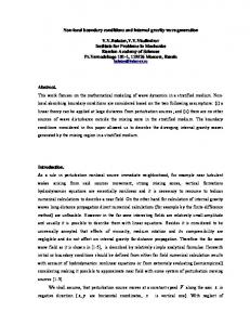
Figure 1. Isosurface of potential temperature with θ = 2.97 within the region of internal gravity wave breaking at (a) t = 62.5, (b) 65, (c) 67.5, and (d) 70.

3. Overview of enstrophy and vorticity evolution In this section, we provide an overview of the evolution of enstrophy and the emergence of coherent vortices within the breaking wave. To begin, the evolution of the breaking wave is illustrated by an isosurface of potential temperature at four times in figure 1, with the wave propagating to the right. This particular isosurface is shown because it resides within the region of vigorous wave breaking. Recalling that a buoyancy period is Tb = 14 in our non-dimensional units, we see that the entire interval displayed spans less than a buoyancy period; this evolution is both more rapid and more vigorous than was observed in our previous lower-resolution, more-viscous simulations. In the first stage of evolution of the breaking wave, regions of convective instability arise (see e.g. the overturning isosurface at t = 65.0 in figure 1) from both a compression of the vertical wavelength and an increase of the wave amplitude with height, due to a decrease in wave intrinsic frequency and mean density with upward propagation. This convective instability results in the formation of streamwise counter-rotating vortex pairs which cause a transition from two- to three-dimensional flow. These vortex pairs are visible in figure 2, which shows a volumetric rendering of the λ2 eigenvalue discussed in § 2.3. The entire wave field is shown (viewed from below with streamwise to the right and spanwise down at several times. Strong vortices are coloured by opaque yellow/green and weaker vortices are coloured by less-opaque blue. The streamwise vortex pairs are visible beginning at t = 62.5 as the ghostly white streaks. As will be discussed in the next section, the streamwise vorticity arises both from direct baroclinic generation of streamwise vorticity and from tilting spanwise shear vorticity into the streamwise direction. The former source dominates at early times, while the latter dominates at later times. This supports the observations of Fritts et al. (1994, 1996b) that the major sources of instability kinetic energy are a

34

Ø. Andreassen, P. Ø. Hvidsten, D. C. Fritts and S. Arendt

(a)

(b)

(c)

(d)

Figure 2. Volume renderings of λ2 viewed from positive x and below showing λ2 at (a) t = 62.5, (b) 65, (c) 67.5, and (d) 70. Colour and opacity scales are such that large negative values are yellow and opaque, and small negative values are blue and less opaque.

conversion from eddy† gravitational potential energy at early times and a conversion from shear kinetic energy at later times. The influences of the streamwise vortices on the isosurfaces of potential temperature can be seen in figure 1 in the panels at t = 62.5 and 65, where downward and upward displacements of the potential temperature surface occur inside and outside vortex pairs respectively. In the next phase of the evolution, the streamwise vortices stretch and tilt the spanwise vorticity of the shear (both the background shear and the shear of the wave itself). Figure 3 shows the enstrophy of the full domain at t = 65 and t = 70. Two views of each are shown: from positive x and above on the right, and from below on the left. High values of enstrophy (|ω 2 | ∼ 15–35 at t = 65.0 and |ω 2 | ∼ 50–150 at t = 70.0) are bright pink and opaque and low values (|ω 2 | ∼ 4–15 at t = 65.0 and |ω 2 | ∼ 4–50 at t = 70.0) are blue and nearly transparent. Enstrophy below 4.0 is not shown. Considering t = 65 first, note that there is significant enstrophy which is not represented in λ2 (compare figures 2b and 3a); this is because most of the enstrophy in figure 3 lies in sheets, as can be seen by comparing figures 3(a) and 3(b), and so does not have the rotational character required to appear in λ2 . Similarly, a careful examination shows that the enstrophy of the streamwise vortices shown in figure 2 at t = 65.0 is too weak to appear in figure 3. In fact, the enstrophy shown in figure 3 at t = 65 has vorticity predominantly in the spanwise direction, and represents the vorticity of the total shear. The vorticity is strong and positive at lower z where the wave shear is in the same direction to the background shear, and is weak and negative at higher z where the wave shear is in the opposite direction as the background shear. It has attained its spanwise-localized sheet shape in the following way. Prior to the appearance of the streamwise vortices, the spanwise vorticity due to the shear has no spanwise structure; it varies only in the streamwise and vertical directions. The streamwise vortices created by the convective instability then advect † The term eddy refers to the field with the spanwise average subtracted.

Vorticity dynamics in a breaking internal gravity wave. Part 1 (a)

(c)

35

(b)

(d)

Figure 3. Volume renderings of enstrophy viewed from below with positive x (streamwise) to the right in the left panels (a, c), and viewed from positive x and above in the right panels (b, d); (a, b) show t = 65 and (c, d) show t = 70. Enstrophy is shown with large values opaque and pink and weak values transparent and grey.

and stretch the spanwise vorticity in their flow. Note, in particular, the shape of the enstrophy in figures 3(a) and 3(b) at t = 65. The areas of brightest pink are strong regions of enstrophy with vorticity in the positive spanwise direction that have been advected downward by the convective rolls. As they are advected downward, their spanwise vorticity is stretched because the flow of the convective rolls diverges in the spanwise direction and so contributes to the straining term in (2.9). This amplifies the enstrophy advected downward over the background enstrophy, and makes the amplified regions thinner since the flow of the convective rolls is convergent in the vertical direction. Interspersing the regions of strong downward-advected enstrophy are regions of enstrophy that have been advected upward and have also been amplified by stretching. These regions, which have negative spanwise vorticity, are weaker than the downward-advected regions because the mean and wave shear are of opposite sign at this phase of the wave. The enstrophy at each wave phase is concentrated in sheets of spanwise vorticity with streamwise extents of roughly 10–20 sheet thicknesses, and spanwise widths of roughly 6 sheet thicknesses. The enstrophy sheets are unstable to the Kelvin–Helmholtz (KH) instability and roll up into a series of vortex tubes. The beginning of one of these roll-ups is visible in figure 3(a) in the topmost vortex sheet on the left side of that panel. That sheet is rolling up into four vortex tubes, all of which are curved in the same manner. This curvature is easily explained by noting that the edges of the original sheet are curved upward (see e.g. figure 3b), and so the ends of the rolled-up tubes lie above their centres. The mean shear flow (which, of course, is partially due to the tubes themselves) advects the tube ends downstream and rotates the curvature of the tubes. At the later time t = 70, all the sheets have rolled up into tubes. Noting that

36

Ø. Andreassen, P. Ø. Hvidsten, D. C. Fritts and S. Arendt (a)

(b)

(c)

Figure 4. Enstrophy (pink) and λ2 (yellow) in a subdomain in the upper left corner of figures 2 and 3 at t = 65. Parts (a) and (b) display side and bottom views with positive x to the left in each case. Part (c) shows a cut-away side view of λ2 (yellow) and a thin sheet of potential temperature in purple and white.

the dynamical timescale of a shear layer is t ∼ (dU/dz)−1 = ω −1 which is roughly t ' 0.2 for a typical vortex sheet, we see that the roll-up of the sheet takes about 10 shear timescales. This can be seen in figure 3, or in figure 2 which has finer time divisions. The resulting vortex tubes are clearly visible in figure 2 showing the λ2 eigenvalue. This KH instability (which we call the secondary instability as it follows and is triggered by the primary convective instability), then, is a distinct and robust feature of the flow which rolls all the vortex sheets into vortex tubes which then form intertwined horseshoe-shaped vortex loops. In figures 2 and 3, note that the enstrophy and vortex fields are advected toward larger x (to the right) by the mean streamwise motion so that the fields are translated by ∼ 1/3 of the domain length from t = 65 to 70. Because of the streamwise shear flow, however, the advection is weaker at lower

Vorticity dynamics in a breaking internal gravity wave. Part 1

37

levels (foreground of figure 2), with the lower structures moving more slowly toward larger x. To show the KH instability in the enstrophy sheets in greater detail, figure 4 displays several views of three vortex loops on one vorticity sheet in the upper central portion of the image at t = 67.5 in figure 2. Figure 4(a) shows the enstrophy (in red/orange for values over 9.0) and λ2 (in blue) viewed from below with positive x (streamwise) to the left; Figure 4(b) shows the same viewed from positive x and y. Figure 4(c) displays a slice through the three vortex loops and shows λ2 (in yellow/green) as well as a surface of potential temperature (with red above, white in the middle and purple below). Here, positive x (streamwise) is to the right. Figure 4 emphasizes the relationship between the vortices and the enstrophy distribution, with the vortices coaligned with the enstrophy maxima. The successive billows are spaced approximately uniformly, and resemble those seen in purely two-dimensional geometries, but have some differences. One difference is the horizontal scale at which the instability occurs. In a two-dimensional flow, the maximum instability occurs for a wavelength of ∼ 7 times the shear layer thickness. In our vortex sheets, however, this scale is approximately 5.0±0.5 times this thickness, where we define the thickness as the full width of the vorticity distribution at 42% maximum, following the convention used for a sech2 (z/d) shear. This difference is possibly a consequence of the localized extent of the vortex sheet, and/or the curvature of the sheet. Figure 4 also shows the detailed shape of the resulting vortex tubes; the tubes are curved, reflecting the curvature of the vortex sheet from which they formed, and their ends are stretched out by the shear. The ends of the tubes intertwine with the ends of neighbouring tubes (see figure 4c) as well as with the original streamwise vortices that intensified and curved the sheets. When the ends of the tubes are sufficiently stretched, the tubes form horseshoe vortices, inclined at an angle of about 45◦ , although this angle varies among the vortices and also changes with time for any given vortex as the vortices evolve and interact. This is broadly consistent with Gerz (1991) who found horseshoe vortices inclined at an angle of about 36◦ , again with some scatter. The net result of the primary convective and secondary dynamical (KH) instabilities is a collection of intertwined vortex loops having counter-rotating streamwise ‘legs’ inclined along the phase of the wave motion and having centres with positive spanwise vorticity (see figure 2d). Successive loops (toward negative x or upstream) have their streamwise legs above and within the adjacent downstream (toward positive x) loops. The result is a complex vorticity field having many sites where vortices with approximately parallel, antiparallel, or orthogonal alignments occur in close proximity and interact strongly. The vortex loops bear a close resemblance to the ‘horseshoe’ and ‘hairpin’ vortices that arise in turbulent boundary layer flows (Acarlar & Smith 1987; Robinson 1991; and Sandham & Kleiser 1992), in stratified and sheared turbulence (Gerz et al. 1994), and in rotating shear flows (Metais et al. 1995). The dynamics of these structures, then, may have implications for the evolution of a broad class of flows.

4. Sources of instability vorticity In this section we examine the vorticity sources accounting for the enstrophy and vorticity distributions described above. This perspective is quite different from the energetics discussion provided by Fritts et al. (1996a, b) and yields a clearer understanding of the origins of and interactions among the instability structures.

38

Ø. Andreassen, P. Ø. Hvidsten, D. C. Fritts and S. Arendt

(a)

(b)

(c)

(d)

Figure 5. A subdomain in the middle of the right edge of the domain shown in figure 2(a). Shown is the correlation of streamwise vortices (yellow) with enstrophy (pink) in (a), and with baroclinic sources (red positive and blue negative) in (b). Also shown are enstrophy (white) with the strain source of spanwise vorticity in (c) and the strain source of vertical vorticity in (d). For the sources, several magnitudes of positive (red) and negative (blue) sources are shown.

4.1. Initial convective instability To understand the initiation and evolution of the primary convective wave instability, we consider the major sources of vorticity at an early stage of wave breaking. In exploring our simulation results, we have found that the effects of dissipation at small eddy amplitudes and large eddy scales are negligible; referring to (2.9), the major sources of eddy vorticity are then baroclinic and strain generation. To begin, a thin (y, z) cross-section of a subdomain at large x and at t = 62.5 is displayed in figure 5. This is a cross-section through a pair of the blue vortex cores shown in figure 2(a). Part (a) shows the enstrophy (in white for values greater than 15.0 and red for values between 2.0 and 15.0) and the streamwise λ2 vortex cores (in yellow). The vortex cores are made transparent so that their interiors are visible. Figure 5(b) shows the streamwise vortices in yellow with the baroclinic source of streamwise vorticity with red positive and blue negative. Figures 5(c) and 5(d) show the enstrophy (white) together with strain sources of spanwise and vertical vorticity respectively (red positive and blue negative). Consider first the display of enstrophy and vortices (figure 5a). The vorticity was initially spanwise and lay in two horizontal sheets: an upper, very thin sheet with negative spanwise vorticity, and a lower thick sheet with positive spanwise vorticity.

Vorticity dynamics in a breaking internal gravity wave. Part 1

39

These sheets were deformed from advection by the flow of the vortex pairs, so that the thin sheet now corresponds to the curved red sheets above the bright white regions. The thick sheet corresponds to the thick white horizontal features near the bottom. The shape of the sheets, and its correlation with the yellow streamwise vortices, reflects the fact that the sheets have been advected by the flow of the vortices. For example, in the centre of the panel is a region being advected upward by the flow of the middle pair of vortices. Referring next to the baroclinic sources of streamwise vorticity (figure 5b) whose typical value is 0.5, we see a clear correlation between the streamwise vortices defined by λ2 and the stronger regions of baroclinic generation, implying that the vortices are generated by baroclinicity. In our flow regime, the baroclinic source of vorticity is equivalent to the torque that the buoyancy force places on the fluid. So, if a fluid is convectively unstable, the buoyancy force produces vortices via the baroclinic production term, and the flow of the resulting vortices mixes the unstable region. Thus, it is clear that the streamwise vortices are a convective, or baroclinicly driven, instability, despite the presence of nearby shear sources of eddy kinetic energy described in our previous wave breaking studies (Fritts et al. 1994, 1996a, b). Although it is not shown, the sign of the baroclinic source reverses with depth as a consequence of the reversals of the vertical gradient of potential temperature above and below the convectively unstable layer, i.e. the fluid above and below the region shown is convectively stable. Comparing figures 5(a) and 5(b), we see that the enstrophy sheets due to strong negative and positive spanwise vorticity lie in the convectively stable regions above and below the convectively unstable layer. At later times, the baroclinic sources become increasingly random in their orientation, due to both the restratification of the initial convectively unstable region and the more complex nature of the flow field and the accompanying potential temperature field (see figures 2 and 3, and the discussion by Fritts et al. 1998). In contrast to the baroclinic sources, the strain contributes to the generation of all components of vorticity at early times. Referring to figure 5(c), strain sources of spanwise vorticity due to stretching are seen in the centres of the enstrophy sheets, with a negative source in the negative upper sheet, and a positive source in the positive lower sheet, accounting for the intensification of those sheets. The latter are the vortex sheets which eventually undergo the KH instability, and it is this stretching which strengthens them to the point where they become dynamically unstable. Regions of spanwise vorticity weakening due to tilting of spanwise vorticity into the vertical and scrunching (i.e. vorticity weakening from local flow convergence) of spanwise vorticity occur at locations where the flow of the vortex pair tilts upward, e.g. the blue region in the centre of the lower half of this panel. These regions of tilting are shown better in figure 5(d) which shows the strain sources of vertical vorticity. Sites where there is strong creation of vertical vorticity due to tilting of spanwise vorticity by the streamwise vortices occur at the edges of each sheet, with oppositely signed sources at opposite edges. For example, note that the curved negative vortex sheet in the centre top of the panel has a positive source on the left and a negative source on the right. This pair of sources is caused by the advection of the sheet in the upward flow of the vortices. Since the sheet is deflected upwards in the middle, the vorticity vectors are tilted to point upward on the right of the sheet and downward on the left. Most of the rest of the sources shown in this panel form similar pairs and are from the same process occurring on different sheets. Finally, strain sources of streamwise vorticity were considered in our previous study and have maxima underlying and anti-correlated with the streamwise vorticity (Fritts

40

Ø. Andreassen, P. Ø. Hvidsten, D. C. Fritts and S. Arendt (a)

(b)

(c)

Figure 6. Same subdomain as in figure 4 at t = 65, showing vorticity vectors (blue weak and red strong) seen from below in (a). Parts (b) and (c) show the tilting source of streamwise vorticity and the stretching source of streamwise vorticity respectively. The view is from below in (b) and from positive x and below (c).

et al. 1996). They are thus correlated well with the strain sources of vertical vorticity shown in figure 5(d) and are not displayed here. 4.2. Secondary dynamical instability We saw above that strain sources contribute to all components of eddy vorticity at early times. The stretching component of this source leads to the intensification and thinning of the vortex sheets, while the tilting component reflects the advection of the sheets in the flow of the streamwise vortices. Thinning and intensification of these sheets drives their local Richardson number to values significantly less than the threshold for shear instability, Ri = 0.25, for two-dimensional plane parallel flows, and a shear instability results. However, the vortex sheets have three-dimensional structure in that they are localized in both the spanwise and streamwise directions,

Vorticity dynamics in a breaking internal gravity wave. Part 1

41

and are also curved (see figure 4); hence, the instability structure differs in important respects from the idealized KH instability in two-dimensions. This secondary KH instability with spanwise-localized structure was discussed in our earlier studies of wave breaking using lower resolution and higher dissipation. However, those studies did not consider the detailed vortex dynamics accounting for the structure and evolution of these features. To investigate the manner in which the secondary dynamical instability proceeds, we focus on the three vortices at the upstream (toward small x) end of the vortex sheet seen in the upper right of figure 2(b). These are shown in figure 6 at t = 65. Figure 6(a) shows the vorticity vectors, while figures 6(b) and 6(c) show enstrophy (in white) along with the off-diagonal tilting and twisting (6b) and diagonal stretching (6c) contributions from the strain source of streamwise vorticity. The views are from negative z in figure 6(a) and from negative z and negative y in figure 6(b, c). Vorticity vectors have magnitudes depicted by colour, with blue weak (ω ' 3.0), red strong (ω ' 6.0), and yellow intermediate (ω ' 4.0 − 5.0). Strain sources are shown with red positive and blue negative. Vorticity vectors in figure 6(a) show that the largest vorticity vectors are curved in the same direction as the enstrophy and vortex structures shown in figures 2 and 3. Looking more closely at the vortex sheet between adjacent maxima, however, we note that the curvature of these vectors in the (x, y)-plane has the opposite sense. This is a consequence of the roll-up of the vortex sheet. Since the sheet has finite spanwise extent, the roll-up of the sheet proceeds faster in the spanwise centre of the sheet than at the edges. This twists the vorticity lines and gives the senses of curvature just mentioned. This is displayed in figure 6(b), which shows the strain sources of streamwise vorticity due to twisting. Note that, at a given spanwise location, the sources within the vortex tubes have the opposite sign to the sources outside the tubes. This is just the twisting of the vortex lines described above. For a given streamwise location, the sources are of opposite signs at each spanwise edge of the sheet, since the two edges are twisted with different senses. This twisting and tilting of vortex vectors at the edges of the vortex tubes is important because it leads to the excitation of twist waves on the vortex tubes; these will be crucial for the dynamics of the tubes at later times and are discussed in the companion paper (Fritts et al. 1998) Less obvious, perhaps, are the strain sources of streamwise vorticity due to stretching displayed in figure 6(c). These are generally positive at the positive-y edge of the vortex sheet and negative at the negative-y edge of the vortex sheet. (Ignore for the moment the prominent red curved soures within the vortex tubes where the reverse is true.) Put another way, the stretching sources are of the same sign as the tilting sources within the vortex tubes and are of the opposite sign outside the vortex tubes. This stretching occurs because the vortex sheets and tubes are not strictly horizontal. They are tilted slightly into the vertical and are thus stretched by the vertical shear (both background and wave shear). Returning to the small regions of oppositely signed sources within the vortex loops, these sources are associated with the curvature of the vortex loops. As vortex lines are advected in the flow around a vortex, they are stretched when they are advected toward a larger radius of curvature, and scrunched when they are advected toward a smaller radius of curvature.

5. Enstrophy spectra To illustrate the enstrophy evolution accompanying wave field instability and the subsequent cascade toward smaller scales of motion more quantitatively, we now

42

Ø. Andreassen, P. Ø. Hvidsten, D. C. Fritts and S. Arendt 100

100

(a)

ö2(kx)

10–1

100

(b)

10–1

10–2

10–2

10–2

10–3

10–3

10–3

10–4

10–4

10–4

10–5

10–5

10–5

10–6

10–6

10–6

1

10

100

1

kx

10

(c)

10–1

100

1

kx

10

100

kx

Figure 7. Streamwise wavenumber (kx ) spectra for the component contributions and total enstrophy at times of t = 60 (a), 70 (b), and 80 (c). The streamwise, spanwise, and vertical contributions, ωi2 , for i = x, y, and z, are shown with dash-dotted, dashed, and dotted lines, respectively, at each time. The kx spectrum of total enstrophy is shown with a solid line. Note that the enstrophy associated with the mean shear flow is excluded in this presentation. 100

100

(a)

ö2(ky)

10–1

100

(b)

10–1

10–2

10–2

10–2

10–3

10–3

10–3

10–4

10–4

10–4

10–5

10–5

10–5 10–6

10–6

10–6 1

10

ky

100

(c)

10–1

1

10

ky

100

1

10

100

ky

Figure 8. As in figure 7, but for the spanwise (ky ) component and total enstrophy spectra.

examine the temporal development of the component and total enstrophy spectra and the domain-averaged enstrophy. While we have divided the discussions of the initial convective and dynamical instabilities and the subsequent vortex interactions between this paper and Part 2, the discussion in this section spans the entire evolution. Streamwise and spanwise spectra of the component and total eddy P wavenumber ωi2 , averaged over the upper domain for 0.2 < z2 /z20 < enstrophies, ωi2 and ω 2 = 0.6, are shown at times t = 60, 70, and 80 in figures 7 and 8†. Note that the ky spectra are corrected for the difference in the x and y domain size to permit comparison of spectral amplitudes at the same scales in each direction. These spectra at t = 60 exhibit clear differences. The ky spectra exhibit a series of discrete peaks corresponding to the scales at which the dominant spanwise instabilities (i.e. the streamwise convective rolls) arise (wavenumbers 4, 10, and 16 in figure 7 or 2, 5, and 8 relative to the spanwise domain). The kx enstrophy spectra, in contrast, have their major contributions at † The eddy enstrophy is the enstrophy with the mean and two-dimensional-wave contributions subtracted by taking a spanwise average.

Vorticity dynamics in a breaking internal gravity wave. Part 1

43

2.5 2.0 1.5

ö2 1.0 0.5 0 60

65

70

75

80

Time Figure 9. Temporal evolution of total enstrophy spanning initial wave field instability and the subsequent transition to turbulent flow. Line codes for component and total enstropies are as in figure 7.

somewhat lower wavenumbers, since the convective rolls are much longer than they are wide. In both spectra, the contributions due to spanwise vorticity are dominant at early times because all of the initial (two-dimensional) vorticity is spanwise and projects first onto spanwise eddy scales via stretching. Interestingly, the excess enstrophy associated with spanwise vorticity contributes preferentially at higher kx and lower ky relative to the other components. The differences at small ky are unimportant because all of the amplitudes here are low. However, those at larger kx are more significant and suggest an enhancement due to the KH instabilities that are emerging in the vorticity and enstrophy fields (see figures 2 and 3). By t = 70, the dominant enstrophy contributions for all components have shifted to wavenumbers kx ∼ 2 to 20 and ky ∼ 2 to 30 (in a variance-content form, the peak would occur at a kx for which the slope in figure 7 is −1) with the enstrophies due to each component of vorticity at higher wavenumbers achieving near isotropy. At later times (t = 80), the peaks in the ky spectra corresponding to the streamwise convective rolls are no longer present, as the vortex loops have interacted and driven the flow toward a more chaotic structure. There remain significant anisotropies at lower wavenumbers in the ky spectra, with the spanwise enstrophy dominating the streamwise and vertical enstrophies by factors of 2 and 4 respectively. The domain-averaged component and total enstrophies are shown as functions of time spanning the instability evolution and the subsequent turbulent decay in figure 9. In order to focus on the evolution of the eddy structures, this presentation excludes the enstrophy associated with the mean and two-dimensional wave motions by subtracting a spanwise average. As shown in § 4.1 and § 4.2, at early times the most significant contribution is that due to stretching (and projection onto non-zero spanwise wavenumbers) of spanwise mean and two-dimensional wave vorticity, with comparable, but smaller, contributions in the streamwise and vertical due to tilting and twisting of this spanwise component. Relative contributions of vorticity in the streamwise and vertical directions increase until the maximum enstrophy is achieved at t ∼ 76. At this time, the two horizontal components have exchanged their relative magnitudes, while the vertical component remains smaller by ∼ 30%. The decay of total enstrophy beyond t ∼ 76 indicates that the flux of enstrophy (and energy) from the mean and wave fields into the eddy, or turbulence, field has decreased at later stages and that our simulation has captured the peak in the level of turbulence

44

Ø. Andreassen, P. Ø. Hvidsten, D. C. Fritts and S. Arendt

activity. However, additional discussion of this stage will be deferred until Part 2 which addresses those aspects of the flow evolution.

6. Summary and conclusions We have presented an analysis of the vorticity dynamics accompanying the initial convective instability and secondary dynamical instability of a breaking internal gravity wave simulated with a three-dimensional, high-resolution numerical model. The gravity wave was excited in a lower model domain and propagated into a higherresolution upper domain having a streamwise wind shear designed to confine wave instability to the domain interior. Open boundary conditions permitting outward propagation of wave energy were used at the lower and upper boundaries of the lower and upper domains, respectively, and periodic boundary conditions were used at the lateral boundaries. Model parameters were chosen to be representative of wave propagation and instability in the middle atmosphere. Our simulation thus describes a common means by which turbulence arises in geophysical flows. Our previous studies at lower resolution examined the energetics of the wave breaking and instability processes and the transports of energy and momentum within the motion field. An important component of this evolution is the vertical transport of momentum by the gravity wave at early times. This transport leads to the formation of a layer of large spanwise vorticity along and below the unstable phase of the wave motion and establishes the initial environment for the vorticity evolution described in this paper. Initial convective instability within the wave field proceeds through the development of streamwise counter-rotating vortices arising due to baroclinic vorticity generation within the convectively unstable phase of the wave. These streamwise vortices evolve immediately above the large spanwise vorticity due to the superposition of wave and mean velocity shears. Strain due to these streamwise vortices contributes in several ways to the subsequent evolution of the spanwise vorticity layer. Stretching of the spanwise vorticity in regions of spanwise-divergent flow below adjacent streamwise vortices leads to thinning and intensification of this vorticity locally. The streamwise vortices also contribute to the generation of vertical vorticity through tilting the edges of each evolving spanwise vortex sheet. Next, secondary dynamical (Kelvin–Helmholtz) instabilities develop on each of the intensified spanwise vortex sheets, serving to concentrate the spanwise vorticity into vortex tubes. At the edges of each spanwise vortex sheet, tilting of vertical vorticity into the streamwise direction by the developing vortex tubes acts to connect each tube with the two counter-rotating streamwise vortices accounting for the intensification of that vortex sheet. The net result of the initial convective and secondary dynamical instabilities is a series of intertwined vortex loops having increasingly complex geometries and interactions with time. The breaking wave evolves from a highly anisotropic two-dimensional initial flow with eddy enstrophy initially associated only with the initial streamwise convective and spanwise dynamical instabilities. Initial spectral distributions of enstrophy are likewise highly anisotropic, with significant differences both in the kx and ky spectra and within the component vorticity contributions to each. As the flow evolves toward increasing complexity, the component contributions to each spectrum became comparable; the only persistent differences are at lower wavenumbers where isotropy in the decay stages of turbulence is not expected because of the large-scale mean flow and wave motion still present.

Vorticity dynamics in a breaking internal gravity wave. Part 1

45

This analysis shows that the vorticity evolution both offers a natural perspective from which to understand the evolution of a flow toward smaller scales of motion and complements the understanding obtained from the energetics analysis of the flow. Consideration of vorticity dynamics provides a simple understanding of the initial convective instability, its role in modulation and intensification of the initial spanwise vorticity layer, and the subsequent dynamical instability of the spanwise vortex sheets. Vorticity dynamics is also employed in Part 2 (Fritts et al. 1998) to examine the subsequent evolution of this flow toward isotropic turbulence. This research was supported by the Norwegian Defence Research Establishment, the National Science Foundation under grant ATM-9419151, and the Air Force Office of Scientific Research under grants F49620-95-1-0286 and F49620-96-1-0300. We are grateful to James Garten for assistance in preparing several of the figures used in the paper.

REFERENCES Acarlar, M. S. & Smith, C. R. 1987 A study of hairpin vortices in a laminar boundary layer. Part 2. Hairpin vortices generated by fluid injection. J. Fluid Mech. 175, 43–83. Andreassen, Ø., Anderson, B. N. & Wasberg, C. E. 1992 Gravity wave and convection interaction in the solar interior. Astr. Astrophys. 257, 763–769. Andreassen, Ø., Lie, I. & Wasberg, C.E. 1994a The spectral viscosity method applied to simulation of waves in a stratified atmosphere. J. Comput. Phys. 110, 257–273. Andreassen, Ø., Wasberg, C. E., Fritts, D. C. & Isler, J. R. 1994b Gravity wave breaking in two and three dimensions, 1. Model description and comparison of two-dimensional evolutions. J. Geophys. Res. 99, 8095–8108. Betchov, R. 1957 On the fine structure of turbulent flows. J. Fluid Mech. 3, 205-216. Canuto, C., Hussaini, M. Y., Quarteroni, A. & Zang T. A. 1988 Spectral Methods in Fluid Dynamics. Springer. Dunkerton, T. J. 1997 Shear instability of internal inertia-gravity waves. J. Atmos. Sci., in press. Erlebacher, G. & Sarkar, S. 1993 Statistical analysis of the rate of strain tensor in compressible homogeneous turbulence. Phys. Fluids A, 5, 3240–3254. Fritts, D. C., Arendt, S., & Andreassen, Ø. 1998 Vorticity dynamics in a breaking internal gravity wave. Part 2. Vortex interactions and transition to turbulence. J. Fluid Mech. 367, 47–65. Fritts, D. C., Garten, J. F. & Andreassen, Ø. 1996a Wave breaking and transition to turbulence in stratified shear flows. J. Atmos. Sci. 53, 1057–1085. Fritts, D. C., Isler, J. R. & Andreassen, Ø. 1994 Gravity wave breaking in two and three dimensions, 2. Three dimensional evolution and instability structure. J. Geophys. Res. 99, 8109–8123. Fritts, D. C., Isler, J. R., Hecht, J. H., Walterscheid, R. L. & Andreassen, Ø. 1996b Wave breaking signatures in sodium densities and OH airglow, Part II: Simulation of wave and instability structures. J. Geophys. Res. 102, 6669–6684. Fritts, D. C. & Yuan, L. 1989 Stability analysis of inertio-gravity wave structure in the middle atmosphere. J. Atmos. Sci. 46, 1738–1745. Gerz, T. 1991 Coherent structures in stratified turbulent shear flows deduced from direct simulations. In Turbulence and Coherent Structures (ed. O. Metais & M. Lesieur). Kluwer. Gerz, T., Howell, J. & Mahrt, L. 1994 Vortex structures and microfronts. Phys. Fluids A 6, 1242–1251. Herring, J. R. & Kerr, R. M. 1993 Development of enstrophy and spectra in numerical turbulence. Phys. Fluids A 5, 2792–2798. Isler, J. R., Fritts, D. C. & Andreassen, Ø. 1994 Gravity wave breaking in two and three dimensions 3. Vortex breakdown and transition to isotropy. J. Geophys. Res. 99, 8125–8137. Jeong, J. & Hussain, F. 1995 On the identification of a vortex. J. Fluid Mech. 285, 69–94. Jimenez, J. 1994 Hyperviscous vortices. J. Fluid Mech. 279, 169–176.

46

Ø. Andreassen, P. Ø. Hvidsten, D. C. Fritts and S. Arendt

Jimenez, J., Wray, A. A., Saffman, P. G. & Rogallo, R. S. 1993 The structure of intense vorticity in isotropic turbulence. J. Fluid Mech. 255, 65–90. Kelvin, Lord 1880 Vibrations of a columnar vortex. Phil. Mag. 10, 155–168. Lie, I. 1994 Multidomain solution of advection problems with Chebyshev spectral collocation techniques. J. Sci. Comput. 9, 39–64. Lundgren, T. S. 1982 Strained spiral vortex model for turbulent fine structure. Phys. Fluids 25, 2193–2203. Metais, O., Flores, C., Yanase, S., Riley, J. & Lesieur, M. 1995 Rotating free-shear flows. Part 2. Numerical simulations. J. Fluid Mech. 293, 47–80. Robinson, S. K. 1991 Coherent motions in the turbulent boundary layer. Ann. Rev. Fluid Mech. 23, 601–639. Sandham, N. D. & Kleiser, L. 1992 The late stages of transition to turbulence in channel flow. J. Fluid Mech. 245, 319–348. Vincent, A. & Meneguzzi, M. 1994 The dynamics of vorticity tubes in homogeneous turbulence. J. Fluid Mech. 258, 245–254. Wasberg, C. E. & Andreassen, Ø. 1990 Pseudospectral methods with open boundary conditions for the study of atmospheric wave phenomena. Comput. Meth. Appl. Mech. Engrg 80, 459–465. Winters, K. B. & D’Asaro, E. A. 1994 Three-dimensional wave breaking near a critical level. J. Fluid Mech. 272, 255–284. Winters, K. B. & Riley, J. 1992 Instability of internal waves near a critical level. Dyn. Atmos. Oceans 16, 249–278. Yuan, L. & Fritts, D. C. 1989 Influence of a mean shear on the dynamical instability of an inertio-gravity wave. J. Atmos. Sci. 46, 2562–2568.