Tennessee Tech University, Cookeville TN, USA. Email: {nguo, zhu21, assaini21, rqiu}@tntech.edu. AbstractâWideband waveform-level precoding with simple.
Waveform-level Precoding with Simple Energy Detector Receiver for Wideband Communication Nan Guo, Zhen Hu, Amanpreet S Saini, Robert Qiu Department of Electrical and Computer Engineering, Center for Manufacturing Research Tennessee Tech University, Cookeville TN, USA Email: {nguo, zhu21, assaini21, rqiu}@tntech.edu Abstract—Wideband waveform-level precoding with simple energy detector receiver is investigated in this paper. The motivation is to provide a cheap radio network with simple receivers and sophisticated transmitters. The energy detector receiver performs relatively poorly, but waveform-level precoding can be used to compensate for the performance loss. Waveform-level precoding is a transmitter-side processing taking advantage of known channel information. Given channel impulse response (CIR), transmitted waveform can be optimized in some criterion. In this paper the optimization goal is to maximize an equivalent signal-to-noise ratio (SNR) at the receiver, assuming no inter-symbol-interference (ISI). Close-form expressions are derived based on the Park’s empirical model for evaluating the receiver operating characteristic (ROC) of energy-detector. Numerical approach is adopted to handle continuous time signals. Channel data measured in office area is used to obtain numerical results. Performance comparison with time reversal precoding as benchmark shows that the optimal waveform can offer gains of several decibels. Index Terms—Energy detector, waveform optimization, time reversal.
I. I NTRODUCTION Recent advances in miniaturization, low-power electronics and wireless communications, stimulated by increasing demands for automation in home and industrial areas, have triggered tremendous interests in the wireless sensor network (WSN) research, development and deployment. Designing WSNs is a big challenge due to tough constraints and conditions posed by specific applications and environments. Examples of these constraints and conditions include power consumption, node simplicity, node cost, low signal leakage and non-line-of-sight propagation, severe multipath, etc. Mainly due to potentially low implementation complexity, suboptimal reception strategies, such as transmitted reference (TR) [1]–[8] and its variants [9]–[13] as well as energy (or square law) detector [14]–[17], have received increasing attention for complexity and cost constrained wideband applications. These suboptimal schemes are of low-complexity in the sense that no channel estimation is required and they are less sensitive to timing error. Of course, their performances are poor comparing to those of the optimal receivers. One philosophy to use simple receivers without sacrificing overall performance is to shift part of receiver side functions to the transmitter side, i.e., add preprocessing at the transmitter to compensate performance loss, which is meaningful for a centralized network where one powerful central station
communicates with a large number of nodes. In particular, high-bandwidth waveform level precoding is feasible as gigaHertz sampling rate becomes practical. Real-time arbitrary waveform precoding provides a new platform for ultimate performance optimization using channel information. Depending upon the channel information, each pair of transmitter and receiver in the system chooses a transmitted waveform that is optimal in some sense. An example of waveform precoding is time reversal pre-filtering at the transmitter to focus the signal in time at the receiver [18]–[24], where the transmitted waveform is simply a time-reversed version of the channel impulse response (CIR). In such a system the receivers can be very simple, because they do not need special means (like a RAKE combiner) to capture dispersed energy over time, and even equalizers may not be necessary. Waveform precoding can take into account both receive signal-to-noise ratio (SNR) and inter-symbol-interference (ISI). A common shortcoming is that the mentioned simple receivers are not able to work with typical linear equalization techniques, thus they are not suitable for applications when ISI exists apparently. Unlike linear receiver, the equivalent discrete channels of some suboptimal schemes behave nonlinearly, where an equivalent discrete-time channel has data input at one end and it outputs decision statistic plus noise at the other end [17], [24]–[26]. The decision statistic contains a desired signal and a nonlinear ISI component that cannot be well handled by normal linear equalization techniques. This fact suggests the use of some waveform-level channel shortening techniques. In addition, in a rich multipath environment waveform precoding combined with multiple transmitter antennas can focus signal into a spot spatially. This spatial focusing feature can enable spatial division multiple access (SDMA) or enhance physical-layer security without consuming additional radio resources [21], [27], [28]. In this paper, a radio system combining waveform precoding and simple energy detector receiver is considered. Both on-off keying (OOK) and pulse position modulation (PPM) can be adopted as modulation schemes. The receiver uses an integrator to accumulate signal energy. For better performance the signal can be weighted prior to integration and there must be a best weighting function depending on the signal waveform and the noise level [29]–[33]. In fact, implementation of weighting function is not of low complexity and
this contradicts the philosophy of low-complexity receiver design. A relatively simpler weighting method is a gating function which is equivalent to the use of a proper integration interval [17], [24], [34], [35]. A practical implementation of a smart integrator is to control the integrator’s on-duration. Denoted by Rb the symbol rate and consider a received symbol waveform with most of the energy concentrated in an interval TI . If TI < Tb = 1/Rb , then integrating over the interval TI outperforms integrating over the interval Tb , since both gather almost the same amount of signal energy but the latter gathers more noise. This paper tries to answer a fundamental question: given the transmission bandwidth and CIR, what are the best transmitted waveform and the best integration window size? Unlike performance evaluation of a linear receiver, analyzing an energy detector receiver is relative difficult. Park’s model is adopted as an approximate analytical tool to formulate the equivalent SNR. Waveform optimization can be conducted based on this equivalent SNR. However, for arbitrary CIR to find a continuous time closed-form optimal solution is not feasible. Instead, a numerical approach using matrix operation is adopted. This work is to be tested on a realtime wideband radio test-bed. To obtain meaningful and convincing results, measured channel data is used to process numerical results. The rest of the paper is organized as follows. The system is described in Section II. Theoretical analysis is presented in Section III. In Section IV, channel sounding are discussed. Numerical results are provided in Section V, followed by some remarks given in Section VI.
Square Law
BPF
Integration
zk
VT
Fig. 1.
Energy-detector receiver.
where h (t) , t ∈ [0, Th ] is the multipath impulse response that takes into account the effect of the RF front-end including the transceiver antennas. “⊗” denotes convolution operation. n(t) is a low-pass additive zero-mean Gaussian noise with one-sided bandwidth W and one-sided power spectral density N0 , and x(t) is the received noiseless symbol-“1” waveform defined as x(t) = h(t) ⊗ p(t). (4) def
We further assume that Tb ≥ Th + Tp = Tx , i.e. no existence of ISI. An energy detector receiver performs squaring operation, integration over a given time window TI , and threshold decision. Corresponding to the time index k, the k-th decision variable at the output of the integrator is given by Z kTb +TI0 +TI zk = r2 (t)dt (5) kTb +TI0 kTb +TI0 +TI
Z
(dk x(t − kTb ) + n(t))2 dt
=
(6)
kTb +TI0
where TI0 is the starting time of integration for each symbol and 0 ≤ TI0 < TI0 + TI ≤ Tx ≤ Tb . III. WAVEFORM D ESIGN A. Equivalent SNR
II. S YSTEM D ESCRIPTION We limit our discussion to a single-user scenario. Assume the channel remains static during a data burst (say 100µs [8]) and CIR is available at the transmitter. How CIR is obtained is not a task of this paper. An ideal low-pass filter with onesided bandwidth W is placed at the receiver’s front-end. The transmitted signal with OOK modulation is s(t) =
∞ X
dj p(t − jTb ),
(1)
j=−∞
where Tb is the symbol duration, p(t) is the transmitted symbol waveform defined over [0, Tp ], and dj ∈ {0, 1} is j-th transmitted bit. Without loss of generality, assume the minimal propagation delay is equal to zero. The energy of p(t) is normalized and defined as Eb , Z Tp p2 (t) dt = 1 (2) 0
The received noise-polluted signal at the output of the receiver front-end filter is r(t) = h(t) ⊗ s(t) + n(t) ∞ X = dj x(t − jTb ) + n(t), j=−∞
(3)
Analyzing an energy detector receiver as shown in Figure 1 is not as easy as analyzing linear receiver. The decision statistic zk can be approximated as a chi-square or a noncentral chi-square random variable, with 2T W degrees of freedom [36], [37]. A number of approximating models have been proposed to evaluate the performance of receiver operating characteristic (RCO) [38]. When 2T W is large, the chi-square or a non-central chi-square pdfs asymptotically become Gaussian by the central limit theorem. In this case, the required receive SNR and decision threshold can be determined, given the probability of false alarm Pf and the probability of detection Pd [38]. With the notation used in this paper, the received SNR before the square law is expressed as, R TI0 +TI 2 x (t) dt (7) dI = TI0 TI W N0 The ROC formulas based on Gaussian approximation can be extended to handle arbitrary value of 2T W by introducing an empirical loss function C(dI ) [39], [40], with its general form b + dI C(dI ) = , (8) dI where a and b are constants. In the following formula, the loss function links the received SNR and an equivalent SNR
which provides the same detection performance when applied to a coherent receiver, SNReq
= =
=
aTI W dI (9) C(dI ) aTI W d2I (10) b + dI �2 �R T +T 2 TI0I0 I x2 (t) dt (11) R T +T 2.3TI W N02 + N0 TI0I0 I x2 (t) dt
The equivalent SNR SNReq is used as a performance indicator in this paper. The parameters a and b take 2 and 2.3, respectively, the same as Park’s selection in [39].
x = Hp
(22)
and the constraint in the optimization problem 13 can be expressed as, 2 kpk2 Ts = 1 (23) where “k•k2 ” denotes the norm-2 of the vector. Meanwhile assume TI /Ts = NI and TI0 /Ts = NI0 , so the valid entries in x for integration constitute xI as, xI = [xNI0 xNI0 +1 · · · xNI0 +NI ]T
(24)
and EI in Equation 12 can be equivalently shown as,
B. Waveform Optimization In order to get the better performance, the equivalent SNR SNReq should be maximized. Define, Z TI0 +TI EI = x2 (t) dt (12) TI0
For given TI and W , SNReq is the increasing function of EI . So the maximization of SNReq in Equation 9 is equvalent to the maximization of EI in Equation 12. So the optimization problem is shown below, R T +T max TI0I0 I x2 (t) dt (13) R Tp 2 s.t. 0 p (t) dt = 1 In order to solve the optimization problem 13, p(t), h(t) and x(t) will be uniformly sampled and the count-part of the optimization problem 13 in the digital domain will be solved. Assume the sampling period is Ts . Tp /Ts = Np , Th /Ts = Nh and Tx /Ts = Nx . So Nx = Np + Nh . p(t), h(t) and x(t) are represented by pi , i = 0, 1, . . . , Np , hi , i = 0, 1, . . . , Nh and xi , i = 0, 1, . . . , Nx respectively, where, pi = p (its ) (14) hi = h (its )
(15)
xi = x (its )
(16)
So the count-part of Equation 4 in the digital domain is shown as, xi
where (•)i,j denotes the entry in the i-th row and j-th column of the matrix. Thus the matrix expression of Equation 17 is,
= pi ∗ hi Np X = pj hi−j
(17) (18)
j=0
Define, p = [p0 p1 · · · pNp ]T
(19)
x = [x0 x1 · · · xNx ]T
(20)
and Construct channel matrix H(Nx +1)×(Np +1) , � hi−j , 0 ≤ i − j ≤ Nh (H)i,j = 0, else
(21)
2
EI = kxI k2 Ts
(25)
Similar to Equation 22, xI can be obtained by, xI = HI p
(26)
where (HI )i,j = (H)NI0 +i,j and i = 1, 2, . . . , NI + 1 as well as j = 1, 2, . . . , Np + 1. So the count-part of the optimization problem 13 in the digital domain can be expressed as, max EI 2 s.t. kpk2 Ts = 1
(27)
This optimization problem can be solved by Lagrange Multiplier method. Define objective function as, � � 2 J = EI + λ 1 − kpk2 Ts (28) � � 2 2 = kHI pk2 Ts + λ 1 − kpk2 Ts (29) where λ is Lagrange Multiplier. From that, HTI HI p = λp
∂J ∂p
= 0, it is obtained (30)
So the optimal solution p∗ is the eigen-vector corresponding to the maximum eigen-value in eigen-function 30 and p∗ satisfies Equation 23. Furthermore, EI∗ will be obtained. IV. C HANNEL S OUNDING The time domain channel sounding is employed to get h(t). This kind of channel sounding consists of a pulse generator, a signal generator, a low noise amplifier (LNA), a transmitter antenna and a receiver antenna, and a digital sampling oscilloscope (DSO). Figure 2 shows the setup of the time domain channel sounding. The signal generator, the pulse generator and the transmitter antenna constitute the transmitter part and DSO along with the receiver antenna and LNA constitutes the receiver part. The signal generator is used to trigger the pulse generator and the pulse generator generates the pulse that is transmitted through the channel. On the receiver side the signal is amplified by LNA and then displayed and recorded on DSO. A triggering signal from the signal generator is also used to synchronize DSO to
Tx Antenna
Rx Antenna
20 15 Pulse Generator
Digital Sampling Oscilloscope
Low Noise Amplifier
10 Optimal SNReq (dB)
Signal Generator
Trigger Signal
Fig. 2.
The setup of the time domain channel sounding.
5 0 Eb/N0=−3dB −5
Eb/N0=−4dB Eb/N0=−7dB
0.6
−10
Eb/N0=−10dB
0.5 −15
0.4
Eb/N0=−13dB 0
10
0.3
20 30 Integration Time (ns)
CIR
0.2
Fig. 4.
0.1 0
15
Eb/N0=−3dB
Time Reversal SNReq (dB)
−0.4
Eb/N0=−4dB
10
−0.3 0
20
40
60
80
100
Time (ns)
Fig. 3.
CIR.
record the data of the received signal. The tapped-delay-line model of CIR will be estimated using “CLEAN”, a matching pursuit algorithm based on the recorded data from DSO and the noiseless waveform template of the transmitted pulse. Raised-cosine filter is used in this paper to emulate the RF front-end filter including the transceiver antennas, so h(t) can be obtained by convolving CIR and the raised-cosine filter with bandwidth W . V. N UMERICAL R ESULTS Figure 3 shows CIR under investigation in this paper and the energy of h(t) is normalized. W = 1GHz. Ts = 0.025ns, Th = 100ns, Tp = 100ns and TI0 + T2I = 100ns. If the optimal waveform p∗ is transmitted, EI∗ (TI ) and SNR∗eq (TI ) will be obtained. If the transmitted waveform is time reversed h(t), EITIR (TI ) and SNRTIR eq (TI ) will be obtained. Figure 4 shows SNR∗eq (TI ) and Figure 5 shows SNRTIR eq (TI ). For the relatively low Eb /N0 region, the optimal TI is less than 5ns seen from Figure 4 and Figure 5. Increasing TI will introduce more noise and the performance will degrade. For the relatively high Eb /N0 region, we can choose the proper TI such that the larger TI can not bring the obvious increase of SNReq . Let’s define two gains to quantify the performance of optimal waveform using time reversal as benchmark. One is an energy gain, Ge (TI ) =
EI∗ (TI ) EITIR (TI )
(31)
and the other is an SNReq gain, GSNReq (TI ) =
SNR∗eq (TI ) SNRTIR eq (TI )
50
SNR∗eq (TI ).
−0.1 −0.2
40
Eb/N0=−7dB Eb/N0=−10dB
5
Eb/N0=−13dB
0
−5
−10
−15
0
10
20 30 Integration Time (ns)
Fig. 5.
40
50
SNRTIR eq (TI ).
Figure 6 and Figure 7 show the energy gain and SNReq gain respectively. When TI → 0, the energy gain and the SNReq gain approach 1. In this kind of situation, the optimal waveform is the time reversed h(t). So, from peak detection’s point of view, time reversal is the optimal waveform-level precoding. However, when TI increases, the optimal waveform can bring obvious performance enhancement not only for the energy gain but also for the SNReq gain. Define, (33) TI∗ = arg max SNRTIR eq (TI ) TI
SNRTIR eq
If (TI∗ ) is used as the benchmark, then the other SNReq gain is defined as, G∗SNReq (TI ) =
SNR∗eq (TI ) ∗ SNRTIR eq (TI )
(34)
Figure 8 shows G∗SNReq (TI ). In the relatively high Eb /N0 region, the performance of optimal waveform can be improved by a few decibels over the time reversal scheme with optimal integration window when TI for optimal waveform is larger than a certain threshold. While if Eb /N0 is relatively low, the optimal TI for optimal waveform is still needed to get the better performance. VI. C ONCLUSION
(32)
Wideband waveform-level precoding with energy detector receiver has been studied. This work is a part of our effort
4.5
4
4
2 0 SNReq Gain (dB)
Energy Gain (dB)
3.5 3 2.5 2
−2 −4 −6 Eb/N0=−3dB
−8
Eb/N0=−4dB
1.5 −10
Eb/N0=−7dB
−12
Eb/N0=−10dB
1
Eb/N0=−13dB
0.5 −14 0
0
10
20
30 40 50 Integration Time (ns)
60
70
Fig. 8. Fig. 6.
Energy gain.
7 6 SNReq Gain (dB)
10
20 30 Integration Time (ns)
40
50
` ∗´ SNReq gain using SNRTIR TI as the benchmark. eq
R EFERENCES
8
5 4 3
Eb/N0=−3dB Eb/N0=−4dB
2
Eb/N0=−7dB Eb/N0=−10dB
1 0
0
Eb/N0=−13dB 0
10
20 30 Integration Time (ns)
Fig. 7.
40
50
SNReq gain.
in searching for simple-receiver solutions with enhanced performance. Thanks to the empirical loss function, elegant analytical frame has been established, enabling derivation of closed-form optimization results. Numerical results show that performance can be improved by a few decibels over the time reversal scheme with optimal integration window, meaning that time reversal is not the best waveform-level precoding for energy detector receiver. This research suggests that waveform-level precoding can significantly extend the communication range without consuming extra transmitted power. The results of this paper will be verified on the realtime wideband radio test-bed. ACKNOWLEDGMENT This work is funded by the Office of Naval Research through a grant (N00014-07-1-0529), and National Science Foundation through a grant (ECS-0622125). The authors wants to thank their sponsors Santanu K. Das (ONR), and Robert Ulman (ARO) for inspiration and vision. The director of Center for Manufacturing Research (CMR) at TTU (Kenneth Currie) and the chair of ECE (Stephen Parke) at TTU has provided the authors with good support for carrying out this research. P. K. Rajan is helpful in many discussions.
[1] J. Pierce and A. Hopper, “Nonsynclronous Time Division with Holding and with Random Sampling,” Proceedings of the IRE, vol. 40, no. 9, pp. 1079–1088, 1952. [2] C. Rushforth, “Transmitted-Reference Techniques for random or unknown Channels,” IEEE Transactions on Information Theory, vol. 10, no. 1, pp. 39–42, 1964. [3] G. Hingorani and J. Hancock, “A Transmitted Reference System for Communication in Random of Unknown Channels,” IEEE Transactions on Communications Technology, vol. 13, no. 3, pp. 293–301, 1965. [4] N. van Stralen, A. Dentinger, K. Welles, R. Gauss, R. Hoctor, and H. Tomlinson, “Delay Hopped Transmitted Reference Experimental Results,” in IEEE Conference on Ultra Wideband Systems and Technologies, 2002, pp. 93–98. [5] J. Choi and W. Stark, “Performance of Ultra-Wideband Communications with Suboptimal Receivers in Multipath Channels,” IEEE Journal on Selected Areas in Communications, vol. 20, no. 9, pp. 1754–1766, 2002. [6] D. Goeckel and Q. Zhang, “Slightly Frequency-Shifted Reference Ultra-Wideband (UWB) Radio: TR-UWB without the Delay Element,” in IEEE Military Communications Conference, 2005, pp. 1–7. [7] D. Goeckel, J. Mehlman, and J. Burkhart, “A Class of Ultra Wideband (UWB) Systems with Simple Receivers,” in IEEE Military Communications Conference, 2007, pp. 1–7. [8] H. Liu, A. Molisch, S. Zhao, D. Goeckel, and P. Orlik, “Hybrid Coherent and Frequency-Shifted-Reference Ultrawideband Radio,” in IEEE Global Telecommunications Conference, 2007, pp. 4106–4111. [9] M. Ho, V. Somayazulu, J. Foerster, and S. Roy, “A Differential Detector for an Ultra-wideband Communications System,” IEEE 55th Vehicular Technology Conference, vol. 4, pp. 1896–1900, 2002. [10] Y. Chao and R. Scholtz, “Optimal and Suboptimal Receivers for Ultra-wideband Transmitted Reference Systems,” in IEEE Global Telecommunications Conference, vol. 2, 2003, pp. 759–763. [11] S. Zhao, H. Liu, and Z. Tian, “A Decision-Feedback Autocorrelation Receiver for Pulsed Ultra-wideband Systems,” in IEEE Radio and Wireless Conference, 2004, pp. 251–254. [12] N. Guo and R. Qiu, “Improved Autocorrelation Demodulation Receivers based on Multiple-Symbol Detection for UWB communications,” IEEE Transactions on Wireless Communications, vol. 5, pp. 2026–2031, 2006. [13] L. V. and T. Z., “Multiple Symbol Differential Detection for UWB communications,” IEEE Trans. Wireless Commun., vol. 7, pp. 1656– 1666, 2008. [14] Y. Souilmi and R. Knopp, “On the Achievable Rates of Ultra-wideband PPM with Non-Coherent Detection in Multipath Environments,” in IEEE International Conference on Communications, vol. 5, 2003, pp. 3530–3534. [15] M. Weisenhorn and W. Hirt, “Robust Noncoherent Receiver Exploiting UWB Channel Properties,” in International Workshop on Ultra Wideband Systems, Joint with Conference on Ultrawideband Systems and Technologies, 2004, pp. 156–160.
[16] S. Paquelet, L. Aubert, B. Uguen, I. Mitsubishi, and F. Rennes, “An Impulse Radio Asynchronous Transceiver for High Data rates,” in International Workshop on Ultra Wideband Systems, Joint with Conference on Ultrawideband Systems and Technologies, 2004, pp. 1–5. [17] N. Guo, J. Zhang, R. Qiu, and S. Mo, “UWB MISO Time Reversal With Energy Detector Receiver Over ISI Channels,” in 4th IEEE Consumer Communications and Networking Conference, 2007, pp. 629–633. [18] N. Guo, R. C. Qiu, Q. Zhang, B. M. Sadler, Z. Hu, P. Zhang, Y. Song, and C. M. Zhou, Handbook of Sensor Networks. World Scientific Publishing, 2009, ch. Time Reversal for Ultra-Wideband Communications: Architecture and Test-bed, pp. 1–41. [19] M. Fink, “Time Reversal of Ultrasonic Fields. Part-I: Basic principles,” IEEE Transactions on Ultrasonics, Ferroelectrics and Frequency Control, vol. 39, no. 5, pp. 555–566, 1992. [20] A. Akogun, R. Qiu, and N. Guo, “Demonstrating Time Reversal in Ultra-wideband Communications Using Time Domain Measurements,” in 51st International Instrumentation Symposium, 2005, pp. 8–12. [21] N. Guo, R. Qiu, and B. Sadler, “An Ultra-Wideband Autocorrelation Demodulation Scheme with Low-Complexity Time Reversal Enhancement,” in IEEE Military Communications Conference, 2005, pp. 1–7. [22] R. Qiu, C. Zhou, N. Guo, and J. Zhang, “Time Reversal With MISO for Ultrawideband Communications: Experimental Results,” IEEE Antennas and Wireless Propagation Letters, vol. 5, p. 269, 2006. [23] N. Guo, J. Zhang, R. Qiu, and S. Mo, “UWB MISO Time Reversal With Energy Detector Receiver Over ISI Channels,” in IEEE Consumer Commun. and Networking Conf, 2007, pp. 11–13. [24] N. Guo, B. Sadler, and R. Qiu, “Reduced-Complexity UWB Timereversal Techniques and Experimental Results,” IEEE Transactions on Wireless Communications, vol. 6, no. 12, pp. 4221–4226, 2007. [25] K. Witrisal, G. Leus, M. Pausini, and C. Krall, “Equivalent System Model and Equalization of Differential Impulse Radio UWB Systems,” IEEE Journal on Selected Areas in Communications, vol. 23, no. 9, pp. 1851–1862, 2005. [26] M. Pausini, G. Janssen, and K. Witrisal, “Performance Enhancement of Differential UWB Autocorrelation Receivers Under ISI,” IEEE Journal on Selected Areas in Communications, vol. 24, no. 4 Part 1, pp. 815– 821, 2006. [27] R. Wilson, D. Tse, and R. Scholtz, “Channel Identification: Secret Sharing Using Reciprocity in Ultrawideband Channels,” IEEE Transactions on Information Forensics and Security, vol. 2, no. 3 Part 1, pp. 364–375, 2007. [28] M. Bloch, J. Barros, M. Rodrigues, and S. McLaughlin, “Wireless Information-Theoretic Security,” IEEE Transactions on Information Theory, vol. 54, no. 6, pp. 2515–2534, 2008. [29] J. Romme, G. Durisi, I. GmbH, and G. Kamp-Lintfort, “Transmit Reference Impulse Radio Systems using Weighted Correlation,” in International Workshop on Ultra Wideband Systems, Joint with Conference on Ultrawideband Systems and Technologies, 2004, pp. 141–145. [30] Y. Chao and R. Scholtz, “Weighted Correlation Receivers for UltraWideband Transmitted Reference Systems,” in IEEE Global Telecommunications Conference, vol. 1, 2004, pp. 66–70. [31] J. Romme and K. Witrisal, “Transmitted-Reference UWB Systems Using Weighted Autocorrelation Receivers,” IEEE Transactions on Microwave Theory and Techniques, vol. 54, no. 4, pp. 1754–1761, 2006. [32] Z. Tian and B. Sadler, “Weighted Energy Detection of Ultra-Wideband Signals,” in IEEE 6th Workshop on Signal Processing Advances in Wireless Communications, 2005, pp. 1068–1072. [33] J. Wu, H. Xiang, and Z. Tian, “Weighted Noncoherent Receivers for UWB PPM Signals,” IEEE COMMUNICATIONS LETTERS, vol. 10, no. 9, p. 655, 2006. [34] S. Franz and U. Mitra, “Integration Interval Optimization and Performance Analysis for UWB Transmitted Reference Systems,” in International Workshop on Ultra Wideband Systems, Joint with Conference on Ultrawideband Systems and Technologies., 2004, pp. 26–30. [35] Y. Chao, “Optimal Integration Time for UWB Transmitted Reference Correlation Receivers,” in Conference Record of the Thirty-Eighth Asilomar Conference on Signals, Systems and Computers, vol. 1, 2004. [36] H. Urkowitz, “Energy Detection of unknown Deterministic Signals,” Proceedings of the IEEE, vol. 55, no. 4, pp. 523–531, 1967.
[37] D. Torrieri, Principles of Secure Communication Systems. Artech House, Inc. Norwood, MA, USA, 1992. [38] R. Mills and G. Prescott, “A Comparison of Various Radiometer Detection Models,” IEEE Transactions on Aerospace and Electronic Systems, vol. 32, no. 1, pp. 467–473, 1996. [39] K. Park, “Performance Evaluation of Energy Detectors,” IEEE Transactions on Aerospace and Electronic Systems, vol. 14, pp. 237–241, 1978. [40] D. Barton, “Simple Procedures for Radar Detection Calculations,” IEEE Transactions on Aerospace and Electronic Systems, vol. 5, pp. 837–846, 1969.