arbitrary rank and stride. In particular .... rank, assuming the checker can move only diagonally left ...... for our real wavefront programs: Checkerboard, Financial,.
Wavefront template implementation based on the task programming model Antonio J.Dios, Rafael Asenjo, Angeles Navarro, Francisco Corbera and Emilio L. Zapata Dept. of Computer Architecture University of Malaga Malaga, Spain {antjgm, asenjo, angeles, corbera, ezapata}@ac.uma.es
Abstract—A particular characteristic of the parallel wavefront pattern is the multi-dimensional streaming nature of the computations that must obey a dependence pattern. Modern task based programming libraries like TBB (Threading Building Blocks) provide interesting features to improve the scalability of this kind of codes but at a cost of leaving some low level task management details to the programmer. We discuss such low level task management issues and incorporate them into a high level TBB based template that we present in this paper. The goal of the template is to improve the programmer’s productivity to allow a non expert user to easily code complex wavefront problems without worrying about task creation, synchronization or scheduling mechanisms. In our template, the user only has to specify a definition file with the wavefront dependence pattern and the function that each task has to execute. In addition, we describe our experience with the TBB based template when coding four complex real wavefront problems, finding that the programming effort of the user is reduced from 25% to 50% at a cost of increasing the overhead below 5% when compared with manual TBB implementations of the same problem.
I. I NTRODUCTION Wavefront is a programming pattern that appears in important scientific applications such as those based in dynamic programming [1] or sequence alignment [2]. In this paradigm, data elements or cells are distributed on multidimensional grids representing a logical plane or space. Although these elements have to be computed in a given order due to dependencies among them, there is also plenty of parallelism to exploit. One interesting feature of this type of problems is that computations can produce a variable number of independent tasks when the data space is traversed. In a previous research [3] we have explored the applicability of the task programming model in the parallelization of the wavefront pattern. We have found that this pattern fits well with the task programming paradigm for a number of reasons: i) The current state-of-the-art task based libraries (OpenMP 3.0 [4], TBB [5], CnC [6]) provide a programming model in which developers express the source of parallelism using tasks, leaving the burden of explicitly scheduling these tasks to the library runtime, offering this way a more productive programming environment; ii) Tasks are much lighter weight than threads, which allow a more scalable parallel
implementation of real wavefront problems (the workload of a cell use to be small -some floating point operations-); iii) The task schedulers of those library runtimes are based on the work-stealing scheduling algorithm, that leads to better load balancing than an OS thread scheduler, offering that way improved scalability [5]. In our research, we have evaluated the functionalities that each task library provides to the user when programming the wavefront pattern, and we have concluded that TBB offers some advantageous features that allow more scalable and efficient implementations of our pattern, namely the atomic capture of shared variables to control synchronization and the task passing (or task recycling) mechanism which is essential to reduce the task creation and scheduling overheads. However, for non expert parallel programmers, it may be difficult to implement a parallel wavefront algorithm in TBB taking care of task creation, synchronization and task recycling activities. To alleviate these difficulties, we propose a high level template in which the programmer only has to provide the dependence pattern and the actual task computation. The proposed template is built on top of TBB, in a similar style to other TBB templates, like the “parallel for” or “pipeline” ones. These templates main goal is to help programmers to parallelize the algorithm by using very high level constructors, so that an user who is not an expert in a parallel language is able to easily exploit a parallel architecture without worrying about platform details or low level task management mechanisms. So the main focus of this paper is to describe the wavefront template, its use and programmability advantages, as well as to present the specific TBB features that we have exploited in its internal design (Section II). In addition, we have conducted several experiments with real and complex wavefront problems (including an H.264 video decoder) to evaluate the abstraction penalty due to the use of the template, its performance and its “programmability” (Section V). Finally we present some related work (Section VI) and conclusions (Section VII). II. WAVEFRONT T EMPLATE In order to illustrate a basic wavefront code implementation using TBB and how to rewrite it to take advantage of the
proposed wavefront template, we will first consider a simple 2D wavefront problem. It is a classic problem consisting in calculating a function, foo, for each cell of a n × n 2D grid [2], as we can see in the sequential code presented in Fig. 1. In that code, on each iteration of the i and j-loop, cells that were calculated in previous iterations are needed: A[i,j] depends on A[i-1,j] and A[i,j-1] (line 3). For that reason, although the data grid, A, is defined as n × n, the iteration space is [1:n-1, 1:n-1], since the first row and column of A are just initial values. The gs parameter of the foo function is used to tune the workload associate to each cell, such that we can analyze the performance for fine, medium and coarse grain tasks, as we will see in section V. 1 2 3
for (i=1; i n − 1 i=0 otherwise
(1)
where function c(i, j) returns the cost associated with cells [i, j] and f (i, j) is computed as: f (i, j) = min(q(i − 1, j − 1), q(i − 1, j), q(i − 1, j + 1)) + c(i, j)
The Financial problem assumes that given m functions f1 , f2 , ..., fm (each one represents a financial interest function of a bank i) and a positive integer n (the budget), we want to maximize the function f1 (x1 )+f2 (x2 )+...+fm (xm ) with the restriction x1 + x2 + x3 + ... + xm = n where fi (0) = 0(i = 1, .., m). Thus the goal, is to maximize the total financial interest of investing n euros in different banks. The xi values represent the quantity of n to invest in the bank i. Now, to solve the problem we define a m × n matrix I where we keep partial values. The value I(i, j) is computed by eq. 2, getting the solution to the problem in I(m − 1, n − 1). Here, we will identify a task with the computation of I(i, j): ( I(i, j) =
f1 (j) max {I(i − 1, j − t) + fi (t)} 0≤t≤j
if i = 1 otherwise
with [1:m-2,1:n-1]->(1,0:n-j-1), which means two things: • The vectors are associated to cells with coordinates (i,j) that belong to the described region: i has to be in the range [1:m-2] and j in [1:n-1], and • For each one of the cells in the described region, there are n − j dependent cells, identified by vectors (1,0:n-j-1). So, for example, for cell [2,1], the dependent cells are those in the next row (row 2 + 1), and in columns within the range 1 + (0 : n − 1 − 1), so the dependent cells are (3,1), (3,2) and (3,3), if n = 4. As we said, from that dependence vector it is possible to generate the counter matrix, but with an extra initialization time because, for each cell, a loop has to increment the counter of each dependent cell. On the other hand, if the programmer provides the counter information ([2:m-1,1:n-1]=j) a single traverse of the matrix will initialize each counter to the column index value, which is actually the number of arrows reaching each cell (see Fig. 6). In the case of the Floyd algorithm, the sequential algorithm has a k-i-j triple nested loop in which D(i,j) is written in the inner loop body. For the wavefront approach we have removed the “j” dimension from the task space, so each task has to compute the D(i, :) row for each k and i iterations, as we show in Fig. 7. That way, the indices in the task region has been defined as (k,i). In that region, the subregion [0:m-2,k+1] identifies the cells in the superdiagonal due to these cells i=k+1 for k=0:m-2. Besides, the subregion [0:m-2,!(k+1)] represents all the other cells (removing those in the last row), due to in these cases i!=k+1. Note that for this last region, the dependence vector (1,0) applies, since Dk−1 (i, :) has to be ready in order to compute Dk (i, :) according to eq. 3. In addition, vectors (1,-i:m-i-1) associated to the superdiagonal cells, capture the fact that, as indicated in eq. 3, Dk−1 (k, :) is needed for all the i iterations of the iteration k. For example, if k=1, D0 (1, :) is read in all the i iterations. Also note that, as in the Floyd’s serial implementation, the wavfront algorithm can also be computed in place with a two dimensional D array due to Dk values can safely overwrite Dk−1 ones.
(2)
The Floyd’s algorithm [8] uses the dynamic programming method to solve the all-pairs shortest-path problem on a dense graph. The method makes efficient use of an adjacency matrix D(i, j) to solve the problem. The new values of that matrix are computed by eq. 3. Dk (i, j) = min{Dk−1 (i, j), Dk−1 (i, k) + Dk−1 (k, j)} k≥1
(3)
Finally, we have also implement the H.264 decoder. H.264 or AVC (Advanced Video Coding) is a standard for video compression. In H.264, a video sequence have multiples video pictures called frames. A frame has several slices, which are self contained partitions of a frame that contain some number of MacroBlocks (MBs). MBs are blocks of 16 × 16 pixels and are the basics unit for coding a decoding. MBs in a frame are usually processed in scan order, which means starting from the top left corner of the frame and moving to the right, row after row. However, processing MBs in a diagonal wavefront manner satisfies all the dependencies and at the same time allows to exploit parallelism between MBs. In [9] a 2D wavefront version of the H.264 decoder is implemented using Pthreads. In particular, we focus on the tf_decode_mb_control_distributed function where the MBs are processed following the wavefront pattern. With this implementation as a starting point we have recoded this H.264 procedure taking advantage of our wavefront template. In Fig. 6 we show the dependence pattern, counter matrix and corresponding definition file for these four algorithms. Although these definition files are self-explanatory if thoroughly analyzed together with the provided dependence pattern, we will pay attention to some remarkable details. For instance, in the Financial problem, although the data grid is m × n, tasks will be dispatched only for the subregion [1:m-1,1:n-1] (all the cells but those in the first row and column). Also, dependence vectors are described
1 2 3 4 5 6 7
void Operation::ExecuteTask() { int k = GetFirst(); int i = GetSecond(); for (int j=0; j(1,-1);(1,0);(1,1) [1:m-2,0]->(1,-1);(1,0) [1:m-2,n-1]->(1,0);(1,1) //Counter values [1,:]=0 [2:m-1,0]=2 [2:m-1,n-1]=2 [2:m-1,1:n-2]=3
Figure 6.
//Data grid [0:m-1,0:m-1] //Task grid [:,:] //Indices //Dependence vectors [0:m-2,k+1]->(1,-i:m-i-1) [0:m-2,!(k+1)]->(1,0) //Counter values [0,:]=0 [1:m-1,k]=1 [1:m-1,!(k)]=2
//Data grid [0:m-1,0:n-1] //Task grid [1:m-1,1:n-1] //Indices //Dependence vectors [1:m-2,1:n-1]->(1,0:n-j-1) //Counter values [1,1:n-1]=0 [2:m-1,1:n-1]=j
//Data grid [0:h-1,0:w-1] //Task grid [:,:] //Indices //Dependence vectors [0:h-2,1:w-2]->(0,1);(1,-1) [0:h-1,0]->(0,1) [0:h-2,w-1]->(1,-1) [h-1,1:w-2]->(0,1) //Counter values [0,0]=0 [0,1:w-2]=1 [0:h-1,w-1]=1 [1:h-1,0:w-2]=2
Dependence pattern, counters matrix and definition files for four wavefront algorithms
patter described in [9] and [10]. A data grid of h × w macroblocks, MBs, is defined, and a task takes care of each MB. Task dependences are described just with vectors (0,1) and (1,-1). Note that, although de (1,0) and (1,1) dependences also exist, these vectors are not really needed since they are implicit in the sequence (0,1)–(1,-1). The original wavefront code in [9] is a Pthread code with a master thread and a pool of worker threads that wait for work on a task queue. The master thread is responsible for handling the initialization and finalization operations. The dependencies of each MB are expressed by a dependence table. Each time that the dependencies for a MB are satisfied a new task is inserted in the task queue. Synchronization among threads and the accesses to the task pool were implemented using semaphores. However, in our implementation, besides the already discussed definition file, we only need to specify the task body, as shown in Fig. 8. This highly simplify the task of porting the code to TBB, since thanks to the template, we are released of many responsibilities: taking care of pthread/task creation, managing the task queue, synchronizing tasks, to name a few of the them. The H.264 task body of Fig. 8 uses a privatized work space (local_WS) per thread. This means that, although there may be thousand of tasks, in TBB these tasks will be carried out by the running threads, so the maximum number of simultaneous running tasks is equal to the number of
threads. Since this number of threads is much smaller (in TBB it is usually equal to the number of cores to avoid oversubscription overheads), using a privatized work space per thread instead of per task is much more efficient. Thus, the function Get_Local_Workspace (line 4 in Fig. 8) identifies the thread in wich the task is running and the corresponding local work space. Then, some information of the current MB, identified by the GetFirst() and GetSecond() template methods, is copied to the local work space (line 7) and later decoded (line 8). 1 2 3 4 5 6 7 8 9
void Operation::ExecuteTask() { H264mb * curr_MB, * local_WS; local_WS = Get_Local_WorkSpace(); curr_MB = Get_Curr_MB(GetFirst(),GetSecond()); // decode current MB copy_MB_to_WS(local_WS, curr_MB); decode_MB(local_WS); } Figure 8. tation
ExecuteTask() method for the H.264 template implemen-
III. I MPLEMENTATION DETAILS The template has been implemented taking into account that it should support 2D and 3D wavefront
problems. In this scenario and without loss of generality, all tasks are internally identified with an integer, ID, starting at 0. The functions GetFirst(), GetSecond() and GetThird() can be used from a given task to convert its ID in the corresponding task coordinates (typically needed to access the data space). There are also functions GetFirstFromID(ID), GetSecondFromID(ID) and GetThirdFromID(ID), that are used internally if coordinates of task ID are needed. The inverse functions CoordinateToID(i,j) and CoordinateToID(i,j,k) are also available. The internal machinery of the wavefront template is based on the Wave class, the TaskWave template class and the Operation class, derived from the latter and that can be used by the user. This Operation class has three public methods: ExecuteTask() that has to be overridden, as we have seen in figures 5, 7 and 8; GetCounter(ID) and GetDependency(o). The last two are automatically generated from the definition file and included in the wavefront.h, although they may be later modified if the programer realizes that they can be optimized somehow. In the wavefront.h it is also created the wavefront_init() function, which initializes some variables (data grid dimensions, task space frontiers, etc) and initializes a Wave *wavefront object. In the constructor of this object the matrix of counters is allocated and all the counters are initialized inside a parallel loop that traverse all the tasks IDs. In each iteration of this parallel loop, the automatically generated method GetCounter(ID) is called. The GetCounter method generated from the 2D wavefront definition file (Fig. 4), is shown in Fig. 9. As we can see in this figure, the method just return a counter value depending on the coordinates of the corresponding task ID. At the time we are initializing the counter matrix, we also collect in a list the IDs of all the tasks with that counter equal to 0.
in Fig. 5. This run() methods only spawn the ready to dispatch tasks which are in the list we gathered during the initialization. Each running task first executes the ExecuteTask() method and then the internally defined launch one. This launch method is the one that identifies all the dependent tasks, decrement their counters and spawn or recycle into them if they are ready. This process iterates until all the counters are nullified so there are no more tasks to spawn. The identification of the dependen tasks is carried out by iteratively calling the GetDependency(o++) method. In Fig. 10 we show the automatically generated GetDependency(o) method for the 2D wavefront example. As we see, this method first identify the (i,j) coordinates of the calling task. Then, depending on the region in which this task is located, the corresponding vectors specified in the definition file will apply one by one. For example, in the basic 2D wavefront we defined three regions (see Fig. 4) and in the first region there are two vectors. Now, assuming a task is in the first region, each time this task calls the function GetDependency(o++), a dependence vector is applied: (0,1) the first time (o==1) and (1,0) the second one (o==2). For each vector, the resulting task coordinates are checked to validate if they are inside the task space and in that case the ID of the resulting task is returned. Otherwise, INVALID_POSITION is returned pointing out that the task is in one of the task space frontiers and that there are no more tasks in that vector direction. When there is no more vectors to follow in the region, NO_MORE_DEPENDENCIES is returned, so the launch() method realizes that all dependent task have been considered and dispatched when ready. 1 2 3 4 5
1 2 3 4 5 6 7 8 9 10 11 12 13 14
int Operation::GetCounter(int ID){ int i= GetFirstFromID(ID); int j= GetSecondFromID(ID); int counter = 0; if((i==1) && (j==1)) counter= 0; if((i==1) && (j>=2 && j=2 && i=2 && i=2 && j=0, due to INVALID_POSITION is a negative number) and in that cases we decrement the counter value of the task and check if it has been nullified. In that case, if we have not decided to recycle into a previous ready task (line 8), we spawn a new one, or otherwise (line 10) we annotate that we are going to recycle the current task into the new one. Note, that a task is going to recycle into the first ready to dispatch dependent task, so the order in which GetDependency() returns the task is relevant. This is, the dispatching mechanism is biased towards recycling into the first tasks returned by GetDependency and spawning the other ones for later execution. Therefore, dependent tasks that can better exploit the data in the cache of the current task should be returned first by GetDependency() and this can be achieved by adequately ordering the dependency vectors in the definition file. Finally, in line 18, in case that the current task is going to recycle into a new one, we update the ID of the task by the one in which is going to be converted.
wavefront dependences with the provided syntax, it is always possible to write the GetDependency and GetCounter methods from scratch. In the next section we describe the BNF notation of the definition file grammar, and the code generator that translate a definition file into the corresponding wavefront.h header file. IV. D EFINITION FILE SYNTAX In Fig. 12 we see the BNF for the definition file syntax. The first rule in line 1 points out that the description file has a “Data Grid” line, a “Task Grid” one, an “Index” line, one or more “Dependency vectors” and zero or more “Counter values” definitions. 1
2 3 4 5
6 7
8 9 10
11 12 13 14 15 16
1
2 3 4 5 6
7 8 9
10 11 12 13 14 15 16 17 18 19 20
template int Wave:: launch(task *t1){ TaskWave * t = (TaskWave*) t1; int IDRecycledTask = -1; int o=1; int IDdepTask= t->getDependency(o++); while(IDdepTask>=0 || (IDdepTask==INVALID_POSITION )){ if ((IDdepTask>0) &&(--counters[IDdepTask]==0)){ if (IDRecycledTask>=0){ t->spawn( *new( this->allocate(t) ) TaskWave(this,IDdepTask) ); }else{ // no recycled task yet t->recycle_as_child_of(*t->parent()); IDRecycledTask = IDdepTask; } } IDdepTask = t->getDependency(o++); } if (IDRecycledTask>0) t->ID = IDRecycledTask; return IDRecycledTask; } Figure 11. The launch() method checks the counters and spawns or recicles into new tasks.
That explained, if the programmer does not like to start from the definition file or it is difficult to express the
:: = \n \n < Index> \n +( \n) *( \n ) :: = :: = ::= [, ] ::= | : | : : | : ::= < + , + > ::= | | < RegionesDep> ::=+|+|+ ::= (, ) ::= (,) | (,) ::= -> ::= ; ;| ; ::= = ::=a|b..|y|z ::= 0|1..|8|9 ::= *|+|-|/|% Figure 12.
Syntaxis of the definition file for 2D wavefronts in BNF
V. E XPERIMENTAL R ESULTS We conduct two main set of experiments, the first one to validate the efficiency of our template implementation and the second one to evaluate the template programmability. We have used as benchmarks the basic 2D, Checkerboard, Financial, Floyd and H.264 previously described codes. A. Template Overhead For these experiments, we have used a multicore machine with 8 cores, where each core is an Intel(R) Xeon(R) CPU X5355 at 2.66GHz, being SUSE LINUX 10.1 the Operating system in the target platform. The codes were compiled with icc 11.1 -O3. We executed each code 5 times and computed the average execution time of the runs to get the execution times. Then, we computed the speedups, that are calculated with respect to the sequential code time. In a first experiment, we analyzed in detail the behavior of the template for our basic 2D wavefront running example. In particular, the goal of this experiment was to evaluate the scalability of our template for different task
granularities. In Fig. 13 we can see the speedups for two implementations of the 2D code and three task granularities: i) TBB-Fine, TBB-Medium and TBB-Coarse represent the speedups for the manual TBB implementation (see Fig. 3) that was used as baseline; ii) Template-Fine, Template-Medium and Template-Coarse represent the speedups for our TBB Template implementation (details are shown in Fig. 5. In the experiments, the granularity of a task is controled by the gs parameter of the foo function (line 3 in Fig. 1). That parameter set the number of floating point operations per task: Fine granularity represents 200 FLOP, Medium 2,000 FLOP and Coarse 20,000 FLOP. In all the cases, the matrix data has 10,000 × 10,000 cells. From the results of Fig. 13, we clearly see that the greater the granularity, the better the scalability of the codes (both manual and Template versions). Besides, we can see that the differences of performance in both implementations are small. Similar results were obtained for other matrix data sizes. Speedups of TBB manual vs. Template in 2D code
Figure 13. Speedup for the basic 2D wavefront codes for different task granularities (200, 2,000 and 20,000 floating point operations). The x-axis represents the number of cores
Fig. 14 represents now the overhead due to the Template for our 2D code and the different granularities. The overhead is computed as the ratio between the difference of times of the template and manual version vs. the time of the manual version. In other words, the increasing of time regarding the optimized manual version. As we can see in the figure, the overhead is not significant for the coarse, even the medium granularity cases (less than 2%). However, in the fine granularity case, the overhead due to the Template may increment the execution times from 6% to 9%. More in detail, in Fig. 15 we show the contribution to this overhead, due to the different stages of our template (see Fig. 5): the initialization (wavefront_init method, line 12) and the computation (wavefront_run method, line 13) stages. Clearly, the computation stage represents the main source of overhead on any granularity case. This overhead is mainly due to the method call costs on that stage. In the next experiment, we focus in the Checkerboard,
Overhead of Template in 2D code
Figure 14. Overhead of the Template for the basic 2D wavefront code for different task granularities (Fine=200, Medium=2,000 and Coarse=20,000 Floating Point Operations). The x-axis represents the number of cores
Financial and Floyd codes. We selected a data matrix of 1,500 × 1,500 cells for Checkerboard, 300 × 300 elements for Financial and 5,000 × 5,000 elements for Floyd. In the Fig. 16 we show the speedups for two implementations of each code: TBB XXX represents the speedups for the manual TBB implementations whereas Template XXX represent the speedups for the Template versions. Now, from these results we see again that the differences of both implementations are small, although the TBB versions tend to scale better. Again similar results were obtained for other matrix input sizes. We could mention that in all these real problems we found fine to medium grain size tasks (around 100-1,000 FLOP), with load unbalance among the tasks in the Financial and H.264 cases. As pointed in the basic 2D wavefront experiment, the finer the granularity of a task, the poorer the performance of the code. In particular, the Checkerboard corresponds to the case of finer granularity task, what explains the lower scalability. The reason for the poor performance in problems with fine grain was found in the next experiment. We used Vtune (the performance analyzer of Intel [12]) to analyze which functions of the TBB manual version of the problems consumed more time. We got that the degradation of performance in problems with fine grain size (Checkerboard) was because the overhead introduces by the TBB functions spawn (this method is invoked each time a new task is spawned), allocate (it selects the best memory allocation mechanism available) and get_task (this method is called after completing the execution of a previous task). In fact, these methods accounted for more than 6% of the total execution time. In problems with medium or big grain size (Floyd code) the overhead of those functions was smaller and it was far lower than 1% of the total execution time. Now, Fig. 17 represents now the overhead due to the Template for our Checkerboard, Financial and Floyd codes. Again, the overhead is computed as the ratio between the
Fine
Figure 15.
Medium
Coarse
Contributions to the template overhead: the initialization stage and the computation stage. The x-axes represent the number of cores
Speedups of TBB manual vs. Template in real problems codes
Figure 16. Speedup for Checkerboard, Floyd and Financial codes for the manual and Template implementations. The x-axis represents the number of cores
difference of times of the template and manual version vs. the time of the optimized manual version. As we can see in the figure, the overhead of the Template is small, ranging from 5% in the Financial code, to less than 0.5% in the Floyd code. In detail, Fig. 18 illustrates the contributions to the overhead, due to the initialization and computation stages of our template in these codes. Now, the initialization overhead has a very low impact specially for the Checkerboard and Financial codes, because the matrix data for these experiments, and therefore the counters matrices are quite small. Overhead of Template in real code
Figure 17. Overhead of the Template for the Checkerboard, Financial and Floyd codes. The x-axis represents the number of cores
Summarizing, these experiments have shown us that our Template implementation is quite efficient for a variety of wavefront codes. The abstraction penalty of our Template due to the higher level problem management supposes an increasing of the execution times, ranging for 8% of increment for codes with fine grain tasks, to less than 1% of increment of time for codes with a coarse grain tasks. We think these are quite small contributions, provided the Template improves the programmer productivity. This issue will be discussed in Section V-B. In order to evaluate our template with even a more complex and large problem, we conduct a new experiment where we compare two parallel implementations of the H.264 decoder benchmark: the original Pthreads implementation [9] against the version based in our TBB Template. Both H.264 implementations were run in four eight-core Intel(R) Xeon(R) CPU X7550 2.00GHz (32 cores) running SUSE 11.1. The codes were compiled with g++ 4.1. We executed each code version 5 times and computed the average execution time of the runs to get the execution times. In particular, we measured the running times of the MBs decoding section (without CABAC). We executed each code version for different frame resolutions of the same video. The goal was now to evaluate the impact of different problem input sizes on the scalability of each version. In Fig. 19 we see the times (in ms.) for the two versions, in the low resolution (352 × 288 pixels=396 MBs), medium resolution (704 × 576 pixels= 1,584 MBs), and high resolution (1,280 × 720 pixels= 3,600 MBs) input video data. From the results, we see that the overhead incurred due to our template is negligible. Besides, our TBB template implementation has a better scalability behavior for any video resolution. Although for low core counts (1, 2 cores) both implementations have similar times, we see that for higher core counts (12, 16, 32 cores), the performance of the Pthreads implementation tends to degrade faster than our TBB template implementation, specially for the medium and high resolution cases. In these cases, the overhead due to contention on the global Pthreads task queue is one of the reasons of the degradation in the Pthreads implementation, a problem that does not arise in the distributed task queue
Checkerboard
Financial
Floyd
Figure 18. Contributions to the template overhead: the initialization stage and the computation stage in our real problems codes. The x-axes represent the number of cores
model of TBB. Anyway, the lack of scalability, specially for the low and medium resolution cases, is explained by the insuficient workload to keep busy all the cores. B. Template Programmability In this section we discuss our findings regarding our second experimental goal: to evaluate the template Programmability. In other words, how productive from a programmer point of view, is to use our Template to code complex wavefront codes. It is difficult to measure the ease of programming. We follow the methodology proposed in [13], where the authors suggest three quantitative metrics to measure the easy of programming of a code. These metrics are: the SLOC (Source Lines Of Code), the CC (Cyclomatic Complexity) and the PE (Programming effort). When computing the SLOC, comments and empty lines are excluded. This metric is perhaps the more dependent on the user programming style than the other two metrics. In general, we can assume that higher values for this metric can originate more error prone and difficult to maintain code. Regarding the CC, the authors in [14] define this metric as the number of predicates plus one. In a well structured program, higher values for this parameter uses to mean a more complex code. Respecting the PE parameter, it is defined in [15] as a function of the number of unique operands, unique operators, total operands and total operators found in a code. The operands correspond to constants and identifiers, while the symbols or combinations of symbols that affect the value of operands constitute the operators. This metric can be representative of the programming effort required to implement an algorithm. So, a higher value of PE means that it is more difficult for a programmer to code the algorithm. Fig. 20 shows the results of the Programmability metrics for our real wavefront programs: Checkerboard, Financial, Floyd and H.264. We compare the metrics on two implementations of each code: the manual TBB version (see Fig. 3) for the Checkerboard, Financial and Floyd codes or the original Pthreads implementation for the H.264 (see [9]), vs. the version using our Template. The SLOC, CC and PE values are normalized with respect to the corresponding values of the manual implementations. For all the codes, the metrics corresponding to our Template versions, have
always smaller values. For instance, the SLOC, the CC and the PE for the Template codes are typically about 50% below of the corresponding manual TBB implementations, except in the H.264 case, where the PE metric for our Template implementation is about 25% below of the Pthreads version. In any case, these results seem to indicate that we gain some easy of programming when using our Template. In summary, the experimental evaluation performed in this section has show us that the proposed TBB based Template for the wavefront pattern, suppose a productive tool with a low overhead cost, when coding complex applications. VI. R ELATED WORKS There have been several research works that have targeted the problem of parallelizing wavefront problems. In [16] the authors propose the concept of region-based programming and describe its benefits for expressing high level array computations in the context of the parallel language ZPL, being the wavefront pattern a particular case of array computation. Although the definition of the regions in that work is similar to the one we propose in this paper, we differ in the goal: the authors in [16] used the information provided by the regions to identify the communication patterns of the array computations in a distributed memory architecture, whereas in our work we just want to simplify the programmer effort when expressing the data dependence information of the problem. Other authors have addressed the implementation of parallel wavefront problems on heterogeneous architectures such as SIMD-enabled accelerators [17], or the Cell/BE architecture [18]. In these works, the authors have focused on vectorization optimizations and on studying the appropriate work distribution on each architecture, forcing the programmer to deal with several low level programming details. We depart from these works in that we rather focus on higher level programming approaches that release the user from the low level architectural details. Precisely, to free the user from dealing with those low level details, there has been substantial effort invested in characterizing parallel patterns. Patterns may also go by the name “algorithm skeleton”[19], being the wavefront one of these patterns [2]. In this research line, there have
Low Resolution: 352 × 288
Figure 19. of cores
Medium Resolution: 704 × 576
High Resolution: 1280 × 720
Time in seconds for the Pthreads and the TBB Template versions of H.264 and different frame resolutions. The x-axes represent the number
Checkerboard
Financial
Floyd
H.264
Figure 20. Program-ability metrics for the Checkerboard, Financial, Floyd and H.264 codes, comparing the manual (TBB) and Template implementations
been a recent proposal [20] in which the authors propose a “wavefront” abstraction for multicore clusters. We differ from this work in that they address specific regular wavefront problems, where the granularity of a computation is very coarse (one cell needs around 117 sec. in a 1Ghz CPU). They use Pthreads and rely on the O.S. scheduler to process the work. On the contrary, our study focus on much more fine task granularity workload, both in regular and irregular problems. A distinguish feature of our work from all the previous related work, is that we propose a wavefront Template in the context of a modern task programming-based library. We identify the low level features of the task programming model needed in the wavefront pattern, and through a high level Template we hide them from the programmer.
case of the H.264 code, the TBB-based template version outperforms the original Pthreads manual version, although in this case thanks to the work-stealing scheduler of the TBB library runtime. Additionaly, we have evaluated the programmability of our template in our four complex codes, using three quantitative metrics that characterize the effort of programming, finding that the template based codes reduce the effort programming metrics from 25% to 50% when compared to the manual versions. Therefore, for the evaluated codes, we conclude that our template is a productive tool with a low overhead cost.
VII. C ONCLUSIONS
[2] J. Anvik, S. MacDonald, D. Szafron, J. Schaeffer, S. Bromling, and K. Tan, “Generating parallel programs from the wavefront design pattern,” Parallel and Distributed Processing Symposium, International, vol. 2, p. 0104, 2002.
The parallel wavefront pattern is an interesting paradigm for which the task based TBB library has no template. Precisely in this paper we propose a TBB based template for this pattern that helps the programmer by hiding the low level task management mechanisms such as: i) the task synchronization through the use of the atomic capture; ii) the task recycling or spawning when a new computation has to be performed; and iii) the task priorization that can exploit the spatial locality. When using our template, the programmer only has to specify a configuration file with the dependence pattern information, and the function that each task has to perform (the ExecuteTask method). Using four complex benchmarks we have found that the abstraction penalty due to the template only supposes at most a 5% of additional overhead when compared to a manual TBB implementation of the same code. Even in the
R EFERENCES [1] V. U. Dasgupta Sanjoy, Papadimitriou Christos, Algorithms. McGraw-Hill Higher Education, 2007.
[3] A. J. Dios, R. Asenjo, A. Navarro, F. Corbera, and E. L. Zapata, “Evaluation of the task programming model in the parallelization of wavefront problems,” High Performance Computing and Communications, 10th IEEE International Conference on, vol. 0, pp. 257–264, 2010. [4] E. Ayguade, N. Copty, A. Duran, J. Hoeflinger, Y. Lin, F. Massaioli, X. Teruel, P. Unnikrishnan, and G. Zhang, “The design of openmp tasks,” IEEE Transactions on Parallel and Distributed Systems, vol. 20, no. 3, pp. 404–418, 2009. [Online]. Available: http://dx.doi.org/10.1109/TPDS.2008.105 [5] J. Reinders, Intel Threading Building Blocks (Scientific and Engineering Computation). O‘Reilly, 2007, http://www.threadingbuildingblocks.org/.
[6] “Intel concurrent collections for c/c++,” http://software.intel.com/en-us/articles/intel-concurrentcollections-for-cc. [7] G. Brassard and P. Bratley, Fundamentals of algorithmics. Upper Saddle River, NJ, USA: Prentice-Hall, Inc., 1996. [8] R. W. Floyd, “Algorithm 97: Shortest path,” Commun. ACM, vol. 5, pp. 345–, June 1962. [Online]. Available: http://doi.acm.org/10.1145/367766.368168 [9] M. A. Mesa, A. Ramirez, A. Azevedo, C. Meenderinck, B. Juurlink, and M. Valero, “Scalability of macroblock-level parallelism for h.264 decoding,” Parallel and Distributed Systems, International Conference on, vol. 0, pp. 236–243, 2009. [10] E. B. V. D. Tol, E. G. T. Jaspers, and R. H. Gelderblom, “Mapping of h.264 decoding on a multiprocessor architecture,” 2003, pp. 707–718. [11] A. Dios, R. Asenjo, A. Navarro, F. Corbera, and E. L. Zapata, “Wavefront template implementations based on the task programming model,” in Technical Report at http://www.ac.uma.es/∼asenjo/research/, February 2011. [12] S. E. S. Programme, “Intel(r) vtune(tm) performance analyzer 8.0.2 for linux,” Mathematical Software Group Rutherford Appleton Laboratory Chilton, Tech. Rep., 2006, http://www.sesp.cse.clrc.ac.uk/. [13] C. H. Gonzalez and B. B. Fraguela, “A generic algorithm template for divide-and-conquer in multicore systems,” High Performance Computing and Communications, 10th IEEE International Conference on, vol. 0, pp. 79–88, 2010. [14] T. McCabe, “A complexity measure,” Software Engineering, IEEE Transactions on, vol. SE-2, no. 4, pp. 308 – 320, dec. 1976. [15] M. H. Halstead, Elements of Software Science (Operating and programming systems series). New York, NY, USA: Elsevier Science Inc., 1977. [16] E. C. Lewis and L. Snyder, “Pipelining wavefront computations: Experiences and performance,” in In Fifth IEEE International Workshop on High-Level Parallel Programming Models and Supportive Environments (HIPS, 1999. [17] O. Storaasli and D. Strenski, “Exploring accelerating science applications with fpgas,” in Proc. of the Reconfigurable Systems Summer Institute, July 2077. [18] A. M. Aji, W.-c. Feng, F. Blagojevic, and D. S. Nikolopoulos, “Cell-swat: modeling and scheduling wavefront computations on the cell broadband engine,” in CF ’08: Proceedings of the 5th conference on Computing frontiers. New York, NY, USA: ACM, 2008, pp. 13–22. [19] J. Falcou, J. Srot, T. Chateau, and J. Laprest, “Quaff: Efficient c++ design for parallel skeletons,” Parallel Computing, vol. 32, no. 7–8, pp. 604–615, 2006, algorithmic Skeletons.
[20] L. Yi, C. Moretti, S. Emrich, K. Judd, and D. Thain, “Harnessing parallelism in multicore clusters with the all-pairs and wavefront abstractions,” in HPDC ’09: Proceedings of the 18th ACM international symposium on High performance distributed computing. New York, NY, USA: ACM, 2009, pp. 1–10.