Wavelet-based Scalable Coding of Still and Time-varying ...

Wavelet-based Scalable Coding of Still and Time-varying Stereoscopic Imagery

Sumit K. Nath Supervisor: Dr. Eric Dubois

School of Information Technology and Engineering (S.I.T.E), Faculty of Graduate and Postdoctoral Studies, University of Ottawa, 880 King Edward Avenue, Ottawa ON - K1N 6N5 Canada

June 2004

Thesis submitted in partial fulfillment of requirements for the degree of Doctor of Philosophy. c 2004 Sumit K. Nath

i

Abstract This thesis addresses the issue of encoding and decoding still and time-varying stereoscopic imagery. A review of current encoding techniques is undertaken, with special emphasis on algorithms having SNR and spatial scalability. A stereo image pair consists of two views of the same scene. Due to the redundant nature of both views, prediction-based techniques produce superior results when compared with independent encoding of both images. Some of the most widely used embedded still-image coding techniques rely on discrete wavelet transform (DWT)-based analysis. However, these schemes cannot be adapted in a straightforward manner to encode stereoscopic still-image pairs. In this thesis, a novel DWT-based embedded stereoscopic still-image codec structure is proposed. This scheme preserves the progressive transmission capability of still-image coding algorithms, while suitably adapting to the nuances and special characteristics of stereoscopic imagery. A comparative study of variable-block and fixed-block disparity estimation is also undertaken. Partition artifacts result due to imperfect disparity compensation. Drawbacks in existing compensation techniques are discussed and a novel loop-filtering scheme is proposed. This is used to smooth disparity-compensated images before generating and subsequently encoding residual images. As seen from this thesis, this scheme improves on the performance of current techniques. In addition, the dyadic sampling structure of a 2-D DWT is exploited to obtain discrete levels of spatial-scalability and forms part of an embedded scheme for transmission of stereoscopic still-images at different spatial resolutions. The proposed algorithm is suitably modified to encode time-varying stereoscopic imagery. Drawbacks of current moving-picture hierarchies are analyzed and a novel hierarchy is proposed that insures that a user has the flexibility to view a sequence either in monoscopic (default) or stereoscopic modes. Independent objective results, explaining SNR and spatial scalability features, are presented when encoding a few pictures of a stereoscopic moving image sequence. In addition, informal subjective results are presented when viewing encoded versions a time-varying sequence.

ii

Acknowledgment “The secret to creativity is knowing how to hide your sources” Albert Einstein

I would like to graciously acknowledge the following individuals who have, directly and indirectly, helped me during the course of this research. It is rightly said that the difference between ordinary and extraordinary is just a little extra. This sums up my work under the supervision of Dr.

Eric Dubois. His patience

and unrelenting zeal for perfection has helped me in raising the standard and outlook of the research work presented in this thesis. I would also like to thank Dr.

James

Walker at the University of Wisconsin, Eau Claire for useful discussions pertaining to the ASWDR algorithm. I would also like to acknowledge Dr.

Tam´ as Frajka for the

(FZ) results presented in Chapter 5. In addition, I would like thank Rahul Shukla at EPFL, Switzerland for the (RS) results presented in the same chapter. The display of stereoscopic moving image sequences, discussed in Chapter 7, was made possible by my colleague Xiaodong Huang at the VIVA Laboratory. I would also like to thank my other colleagues at the VIVA laboratory who have helped me in various miscellaneous aspects during the course of this research work. The “angioMR” stereo image pair has been provided by Dr.

Thomas Langø at SINTEF Unimed, Trondheim, Norway. Source

codes for the ASWDR algorithm was provided by Dr.

James Walker .

In addition, this thesis would not have appeared in its current shape without the help and support of the following individuals. I would like to extend my gratitude to my good friend Mr.

Andreas Moser for his help and support that made my arrival in Canada

possible. I would also like to thank Dr.

Jayanta Kumar Ray and Mr.

Rakesh A.

Nayak for their help and support during my stay in Calgary. I will always be indebted to my good friends Rohini and Katla Chandrasekhar for their support at various stages of this thesis. I would also like to extend the same feeling of indebtedness to my friend Ravi Sridhar Murthy . I would also like to my friend Mr.

Kulbhushan

iii Kapoor and his extended family. They have been a surrogate family and have made my stay in Ottawa very worthwhile. In the same vein, I would like to thank Mr.

G´ erald

Levert and his family. Last but not the least, I will always be indebted to my Mama and Mami in Calcutta, India for their emotional support throughout the course of this research.

iv

Contents 1 Problem Definition and Thesis Scope

1

1.1 Background information . . . . . . . . . . . . . . . . . . . . . . . . . . .

1

1.2 Summary of proposed research work . . . . . . . . . . . . . . . . . . . . .

5

1.2.1

Problem definition . . . . . . . . . . . . . . . . . . . . . . . . . .

5

1.2.2

Justifying the proposed research work . . . . . . . . . . . . . . . .

7

1.3 Thesis organization . . . . . . . . . . . . . . . . . . . . . . . . . . . . . .

11

2 Preliminaries on Stereoscopic Imaging and Wavelets

14

2.1 Concepts of stereoscopic imaging . . . . . . . . . . . . . . . . . . . . . .

14

2.2 Wavelets and multiresolution analysis . . . . . . . . . . . . . . . . . . . .

19

2.3 Summary of disparity- and motion-estimation algorithms . . . . . . . . .

26

2.3.1

Justification for disparity and motion estimation in stereoscopic moving-image coding . . . . . . . . . . . . . . . . . . . . . . . . .

2.3.2

26

Summary of relevant algorithms for disparity- and motion-estimation 27

2.4 Hierarchical-search strategy . . . . . . . . . . . . . . . . . . . . . . . . . 3 Adaptively-Scanned Wavelet-Difference-Reduction Algorithm

30 34

3.1 Progressive coding of still images . . . . . . . . . . . . . . . . . . . . . .

34

3.2 Summary of wavelet-based image coding schemes . . . . . . . . . . . . .

36

3.3 Justification of using an adaptively-scanned wavelet-difference-reduction algorithm . . . . . . . . . . . . . . . . . . . . . . . . . . . . . . . . . . .

39

Contents

v

3.4 Steps implemented in an ASWDR algorithm . . . . . . . . . . . . . . . .

40

3.5 An example . . . . . . . . . . . . . . . . . . . . . . . . . . . . . . . . . .

48

4 Stereoscopic Still-Image Coding - A summary

51

4.1 Introduction . . . . . . . . . . . . . . . . . . . . . . . . . . . . . . . . . .

51

4.2 Solutions for disparity estimation and compensation . . . . . . . . . . . .

53

4.2.1

Disparity estimation . . . . . . . . . . . . . . . . . . . . . . . . .

53

4.2.2

Disparity compensation

. . . . . . . . . . . . . . . . . . . . . . .

55

4.3 Summary of algorithms . . . . . . . . . . . . . . . . . . . . . . . . . . . .

56

4.4 Asymmetrical Coding . . . . . . . . . . . . . . . . . . . . . . . . . . . . .

59

5 Proposed Wavelet-Based Scalable Stereoscopic Still-Image Codec 5.1 Proposed codec . . . . . . . . . . . . . . . . . . . . . . . . . . . . . . . .

65 65

5.1.1

SNR-scalability . . . . . . . . . . . . . . . . . . . . . . . . . . . .

67

5.1.2

Spatial-scalability . . . . . . . . . . . . . . . . . . . . . . . . . . .

70

5.2 Justification for a new loop-filtering scheme

. . . . . . . . . . . . . . . .

73

5.3 Edge-preserving noise-reduction filter . . . . . . . . . . . . . . . . . . . .

75

5.4 Variable-block-based partitioning schemes . . . . . . . . . . . . . . . . .

77

5.4.1

Rate-distortion constrained quadtree-partitioning schemes . . . .

77

5.4.2

Image content based quadtree-partitioning . . . . . . . . . . . . .

80

5.5 Results and analysis . . . . . . . . . . . . . . . . . . . . . . . . . . . . .

83

5.5.1

Performance evaluation when using a loop filter . . . . . . . . . .

5.5.2

Qualitative results when using fixed-block and variable-block dis-

83

parity estimation . . . . . . . . . . . . . . . . . . . . . . . . . . .

85

5.5.3

Experimental results with monochrome images . . . . . . . . . . .

85

5.5.4

Results for encoding stereoscopic color images . . . . . . . . . . . 100

Contents

vi

6 Summary of Stereoscopic Moving-Image Encoding and Decoding Algorithms

110

6.1 Introduction . . . . . . . . . . . . . . . . . . . . . . . . . . . . . . . . . . 110 6.2 Current picture hierarchies and their drawbacks . . . . . . . . . . . . . . 112 6.3 Selected stereoscopic moving-image encoding algorithms

. . . . . . . . . 115

6.4 Temporal interleaving in stereoscopic moving-image encoding . . . . . . . 119 7 Proposed Wavelet-Based Scalable Stereoscopic Moving-Image Codec 121 7.1 New picture hierarchy . . . . . . . . . . . . . . . . . . . . . . . . . . . . 121 7.2 Design characteristics of the proposed codec . . . . . . . . . . . . . . . . 124 7.2.1

SNR-scalability . . . . . . . . . . . . . . . . . . . . . . . . . . . . 124

7.2.2

Encoding color stereoscopic moving-images . . . . . . . . . . . . . 128

7.2.3

Spatial-scalability . . . . . . . . . . . . . . . . . . . . . . . . . . . 130

7.3 Results and analysis . . . . . . . . . . . . . . . . . . . . . . . . . . . . . 131 7.3.1

Experimental results with monochrome images . . . . . . . . . . . 131

7.3.2

Informal results when encoding color stereoscopic moving-image sequence . . . . . . . . . . . . . . . . . . . . . . . . . . . . . . . . 135

7.3.3

Sequences when viewed in monoscopic mode . . . . . . . . . . . . 139

7.3.4

Sequences when viewed in a stereoscopic mode . . . . . . . . . . . 140

8 Conclusion and Future Work

143

8.1 Summary of proposed algorithm . . . . . . . . . . . . . . . . . . . . . . . 143 8.1.1

Stereoscopic still-image coding . . . . . . . . . . . . . . . . . . . . 143

8.1.2

Stereoscopic moving-image coding . . . . . . . . . . . . . . . . . . 145

8.2 Summary of original contributions made in the thesis . . . . . . . . . . . 145 8.3 Scope for future research work . . . . . . . . . . . . . . . . . . . . . . . . 148 A “CDF-9/7”, “Odegard-9/7”, “Cooklet-17/11” - Lifting Steps

150

Contents B ASWDR algorithm - Some Results B.1 Comparison between WDR and ASWDR algorithms

vii 154 . . . . . . . . . . . 154

B.2 Comparison with JPEG2000 and SPIHT . . . . . . . . . . . . . . . . . . 155 C Software, Hardware and CD ROM Details

163

C.1 Software . . . . . . . . . . . . . . . . . . . . . . . . . . . . . . . . . . . . 163 C.2 Hardware . . . . . . . . . . . . . . . . . . . . . . . . . . . . . . . . . . . 163 C.3 CD ROM . . . . . . . . . . . . . . . . . . . . . . . . . . . . . . . . . . . 164 References

165

viii

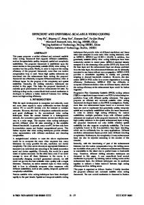
List of Figures 1.1 QoS frameworks for transmission of monoscopic video content in (a) independent and (b) embedded simulcast modes. K1 , K2 and K3 represent bit-rates. . . . . . . . . . . . . . . . . . . . . . . . . . . . . . . . . . . . .

2

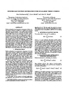
1.2 QoS frameworks for transmission of stereoscopic video content in (a) independent and (b) embedded simulcast modes. K1 , K2 and K3 represent bit-rates. . . . . . . . . . . . . . . . . . . . . . . . . . . . . . . . . . . . .

3

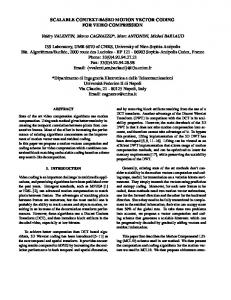
2.1 Schematic of a Binocular Stereoscopic Imaging System. Proper optical arrangements are incorporated so as to prevent inversion of images. Both camera’s are assumed to be stationary. . . . . . . . . . . . . . . . . . . . 2.2 2-channel filter-bank.

. . . . . . . . . . . . . . . . . . . . . . . . . . . .

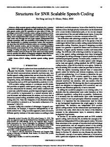
15 20

2.3 1-level, 2-D separable, forward and inverse wavelet transform using Mallat’s algorithm. cm is a 2-D discrete signal.

. . . . . . . . . . . . . . . .

23

2.4 3-scale wavelet decomposition of a 2-D image (having dyadic dimensions), using Mallat’s algorithm. Image dimensions are (M, N ). . . . . . . . . .

24

2.5 Lifting-based implementation of a 1-scale DWT, previously shown in Fig. 2.2 . . . . . . . . . . . . . . . . . . . . . . . . . . . . . . . . . . . . . . .

25

2.6 Block disparity- or motion-vector estimation . . . . . . . . . . . . . . . .

29

List of Figures

ix

2.7 Hierarchical disparity-vector estimation, in a DWT framework. ↑2 indicates a dyadic upsampling performed in a 2-D separable DWT. Disparityestimation is performed between the all low-pass subband at each scale. Disparity-vectors from coarse-scales are scaled by a factor of two, when moving to a finer scale. A similar strategy can be used when estimating motion-vectors. . . . . . . . . . . . . . . . . . . . . . . . . . . . . . . . .

32

3.1 Progressive image coding of wavelet-transformed coefficients. The x-axis indicates magnitudes of coefficients. |T1 | > |T2 |. The y-axis indicates the number of coefficients satisfying a “greater than threshold ” criterion.

. .

36

3.2 Parent-child or inter-scale relationship between wavelet coefficients at different subbands. Coefficients have been scaled for display purpose.

. . .

37

3.3 Intra-scale relationship between wavelet coefficients in any given subband. Coefficients have been scaled for display purpose. The direction of arrows indicate that all coefficients at a particular scale are examined before a coefficient can be deemed significant. . . . . . . . . . . . . . . . . . . . .

39

3.4 Methodology used in an ASWDR algorithm. Significance of coefficients is determined via intra-scale correlation. Inter-scale correlation is used to “bring forward” descendants of previously identified significant coefficients. This reduces overall bits required to encode positions of significant coefficients. . . . . . . . . . . . . . . . . . . . . . . . . . . . . . . . . . . 3.5 Shapiro’s 8×8 image having three levels of wavelet transform

41

. . . . . .

42

3.6 Scan order employed in accumulating coefficients. . . . . . . . . . . . . .

42

4.1 Two distinct stereoscopic still-image coding hierarchies . . . . . . . . . .

54

4.2 Residual error quantization . . . . . . . . . . . . . . . . . . . . . . . . . .

55

List of Figures

x

4.3 Raw and residual versions of an extracted portion from the “basketball ” target (left) image. Images have been scaled for display purposes. . . . .

58

4.4 An example of Gaussian-blurred target image, with a higher perceptual quality reference image. . . . . . . . . . . . . . . . . . . . . . . . . . . . .

60

4.5 Raw target (left view) image and an anaglyph with a full-resolution reference image from the “outdoors” stereo-image pair (dimensions = 640×480). 61 4.5 Medium level of blur applied on the target image, and a corresponding anaglyph with a full-resolution reference image. Target (left) image has been blurred using a 2-D Gaussian filter G(x, y) =

1 2πr 2

e−

x2 +y 2 2r 2

. . . . . .

62

4.5 High level of blur applied on the target image, and a corresponding anaglyph with a full-resolution reference image. Target (left) image has been blurred using a 2-D Gaussian filter G(x, y) =

1 2πr 2

e−

x2 +y 2 2r 2

. . . . . . . . . . . . . .

63

5.1 Block diagram of proposed codec, with SNR-scalability, at a specified spatial-resolution. . . . . . . . . . . . . . . . . . . . . . . . . . . . . . . .

66

5.2 Global structure for spatial scalability . . . . . . . . . . . . . . . . . . . .

71

5.2 contd. The dotted box depicts the procedure in which energy of a residual image at a finer scale is minimized, using a locally decoded version of a residual image from a coarse scale. The modified residual image is encoded and subsequently decoded using an ASWDR encoding/decoding scheme, at a bit-rate of Ki . These are indicated as E(Ki ) and D(Ki ), respectively. A previously encoded residual image, at a coarse scale, is subtracted (X) and subsequently added (Y) to regenerate the residual at the current scale. Other notations are similar to that shown in Fig. 5.1(a). . . . . . . . . .

72

5.3 Overlapped-block disparity compensation (OBDC). All blocks must have same dimensions.

Different regions of the block (enclosed within the

dashed line) are estimated from different neighbours. . . . . . . . . . . .

73

List of Figures

xi

5.4 Examples of region-based disparity-compensation . . . . . . . . . . . . .

74

5.5 Representative examples of quadtree-partitioning schemes . . . . . . . . .

78

5.6 Quadtree-partitioning of Y-component of a textured image, with quadtreemap generated at scale-0 (i.e., at original spatial resolution). Vt = 30. Block dimensions range from 8×8 - 32×32. Image dimensions are 1024×1024. 81 5.7 Image from Fig. 5.6, partitioned using a quadtree-map generated at scale2 (e.g., as in Fig. 2.7) with a threshold Vt = 120. Block dimensions range from 8×8 - 32×32. Image dimensions are 1024×1024. . . . . . . . . . . .

82

5.8 Sections of disparity compensated residual images when encoding the “basketball ” stereo-image pair. The images have been scaled for display purposes. A raw version of this image section can be seen from Fig. 4.3(a). 84 5.9 Residual image obtained when predicting image shown in Fig. 5.7. A 3-scale hierarchical fixed-block-based disparity estimation scheme is used, with scale-0 block size of 16×16. Image has been scaled for display purposes. 86 5.10 Residual image obtained when predicting image shown in Fig. 5.7. A 3scale hierarchical variable-block-based disparity estimation scheme is used, with a scale-0 block sizes ranging from 8×8 - 32×32. Image has been scaled for display purposes. . . . . . . . . . . . . . . . . . . . . . . . . . . . . .

87

5.11 “outdoors”, “fruits” and “arch” stereo-image pairs. . . . . . . . . . . . .

88

5.12 Block structure of “outdoors” and “fruits” target image-views, when using fixed- and variable-block-based disparity estimation. . . . . . . . . . . . .

90

5.13 PSNR plots and residual images at scale-0 when encoding the “outdoors” stereo-image pair. Variable-block-based disparity estimation, 4-scale DWT and EPNR filter (with λ = 1.35 and two filter iterations) have been used. Images have been scaled for display purposes. . . . . . . . . . . . . . . .

99

List of Figures

xii

5.14 4:4:4 RGB to 4:2:0 YCbCr conversion. Cbs and Crs represent downsampled versions of Cb- and Cr-components. . . . . . . . . . . . . . . . . . . 100 5.15 File structure of an encoded color stereo-image pair (independent simulcast mode). . . . . . . . . . . . . . . . . . . . . . . . . . . . . . . . . . . 102 5.16 Representative examples of individual target images (raw and encoded) and anglyphs (raw and encoded) from the “bull ” stereo-image pair. . . . 105 5.16 contd. . . . . . . . . . . . . . . . . . . . . . . . . . . . . . . . . . . . . . 106 5.16 contd. . . . . . . . . . . . . . . . . . . . . . . . . . . . . . . . . . . . . . 107 5.16 contd. . . . . . . . . . . . . . . . . . . . . . . . . . . . . . . . . . . . . . 108 6.1 Encoding and display hierarchy of contiguous pictures in a, MPEG-2 compliant, monoscopic moving-image sequence (GOP = 10). . . . . . . . . . 113 6.2 MPEG-2 complaint multiview picture hierarchy for encoding stereoscopic imagery. . . . . . . . . . . . . . . . . . . . . . . . . . . . . . . . . . . . . 114 6.3 Disparity-compensated multiview picture hierarchy for encoding stereoscopic imagery. . . . . . . . . . . . . . . . . . . . . . . . . . . . . . . . . 114 6.4 Stereoscopic moving-image codec structure proposed by Sethuraman, Siegel and Jordan . . . . . . . . . . . . . . . . . . . . . . . . . . . . . . . . . . 115 6.5 Stereoscopic moving-image encoding structure proposed by Thanapirom, Fernando and Edirisinghe . . . . . . . . . . . . . . . . . . . . . . . . . . 116 6.6 Two-loop, DCT-based SNR-scalable encoder, proposed by Arnold, Frater and Wang. . . . . . . . . . . . . . . . . . . . . . . . . . . . . . . . . . . . 118 7.1 Proposed contiguous picture hierarchy, used in stereoscopic moving-image encoding (GOP = 10) . . . . . . . . . . . . . . . . . . . . . . . . . . . . 122 7.2 Proposed contiguous picture hierarchy, when used in multi-view (i.e., more than 2 views) moving-image encoding (GOP = 10) . . . . . . . . . . . . 123

List of Figures

xiii

7.3 Fundamental Structure employed when encoding different pictures of a stereoscopic moving-image sequence at the highest spatial resolution. . . 125 7.3 cont. . . . . . . . . . . . . . . . . . . . . . . . . . . . . . . . . . . . . . . 126 7.4 Bit-streams of various components when encoding a stereoscopic movingimage sequence at a specific spatial resolution.

e.g., YIPT ar indicates

the Y-component of the disparity compensated residual image between a reference I-picture and a target P-picture. QT Map(.) indicates the quadtree map for the picture that is being estimated. DVX , MVX indicates disparity- and motion-vectors as per notations previously introduced in Chapter 2. . . . . . . . . . . . . . . . . . . . . . . . . . . . . . . . . . 129 7.5 PSNR plots when encoding motion- and disparity compensated residual images with loop-filtering (2), independent ASWDR coding (◦) and without loop-filtering () in an independent simulcast mode. Image dimensions are 704×576. . . . . . . . . . . . . . . . . . . . . . . . . . . . . . . . . . 133 7.6 Comparative PSNR plots when encoding motion- and disparity compensated residual images in independent (2) and embedded simulcast modes (◦). Image dimensions are 704×576. . . . . . . . . . . . . . . . . . . . . . 134 7.7 Residual images when encoding P-pictures from I-pictures. Image dimensions are 704×576. Images have been scaled for display purposes. . . . . 136 7.8 Residual images when encoding B-pictures from I-Pictures. Image dimensions equals 704×576. Images have been scaled for display purposes.

. . 137

7.9 Modified asymmetrical coding frameworks for stereoscopic moving-images. “H” and “L” indicates overall high and low bit-rates when encoding reference and target pictures. . . . . . . . . . . . . . . . . . . . . . . . . . . 138 B.1 Right image-view from the “angioMR” stereo-image pair. Image dimensions equals 384 × 352. . . . . . . . . . . . . . . . . . . . . . . . . . . . . 156

List of Figures

xiv

B.2 Disparity-compensated residual image from the “angioMR” stereo-image pair. Image dimensions equals 384 × 352. Image has been scaled for display purposes. . . . . . . . . . . . . . . . . . . . . . . . . . . . . . . . 157 B.3 Original and ASWDR encoded “Barbara” image. Image dimensions are 512×512 . . . . . . . . . . . . . . . . . . . . . . . . . . . . . . . . . . . . 158 B.4 “Barbara” image encoded with SPIHT and JPEG2000. Image dimensions are 512×512 . . . . . . . . . . . . . . . . . . . . . . . . . . . . . . . . . . 159 B.5 Original and ASWDR encoded “mandrill ” image. Image dimensions are 512×512 . . . . . . . . . . . . . . . . . . . . . . . . . . . . . . . . . . . . 160 B.6 “Mandrill ” image encoded with SPIHT and JPEG2000. Image dimensions are 512×512 . . . . . . . . . . . . . . . . . . . . . . . . . . . . . . . . . . 161

xv

List of Tables 3.1 Output data stream for the matrix shown in Fig. 3.5 using a WDR encoding process. The column on the left indicates the current pass (Di = dominant pass, Si = refinement pass). The column on the right indicates the threshold for the current pass. Boldfaced numbers indicates an occurrence of EOS . . . . . . . . . . . . . . . . . . . . . . . . . . . . . . .

50

3.2 Output data stream for the matrix shown in Fig. 3.5 using an ASWDR encoding process. The column on the left indicates the current pass (Di = dominant pass, Si = refinement pass). The column on the right indicates the threshold for the current pass. Boldfaced numbers indicates an occurrence of EOS . . . . . . . . . . . . . . . . . . . . . . . . . . . . . . .

50

5.1 Ref. (right) view of “outdoors” stereo-image pair encoded at 2.00 bpp. .

92

5.2 Ref. (right) view of “outdoors” stereo-image pair encoded at 5.33 bpp. .

92

5.3 Encoding “outdoors” stereo-image pair with different wavelet filters. Ref. image at 2.00 bpp. . . . . . . . . . . . . . . . . . . . . . . . . . . . . . .

92

5.4 Encoding “outdoors” stereo-image pair with different wavelet filters. Ref. image at 5.33 bpp. . . . . . . . . . . . . . . . . . . . . . . . . . . . . . .

92

5.5 Encoding “outdoors” stereo-image pair with fixed-block (F.B) and variableblock-based (V.B) disparity estimation using “CDF-9/7” filters. Ref. image at 2.00 bpp. . . . . . . . . . . . . . . . . . . . . . . . . . . . . . . . .

92

List of Tables

xvi

5.6 Ref. (right) view of “fruits” stereo-image pair encoded at 2.00 bpp. . . .

93

5.7 Ref. (right) view of “fruits” stereo-image pair encoded at 5.33 bpp. . . .

93

5.8 Encoding “fruits” stereo-image pair with different wavelet filters. Ref. image at 2.00 bpp. . . . . . . . . . . . . . . . . . . . . . . . . . . . . . .

93

5.9 Encoding “fruits” stereo-image pair with different wavelet filters. Ref. image at 5.33 bpp. . . . . . . . . . . . . . . . . . . . . . . . . . . . . . .

93

5.10 Encoding “fruits” stereo-image pair with fixed-block (F.B) and variableblock-based (V.B) disparity estimation using “CDF-9/7” filters. Ref. image at 2.00 bpp. . . . . . . . . . . . . . . . . . . . . . . . . . . . . . . . .

93

5.11 Ref. (left) view of “arch stereo-image pair encoded at 0.25 bpp. . . . . .

94

5.12 Encoding “arch” stereo-image pair with different wavelet filters. Ref. image at 0.25 bpp. . . . . . . . . . . . . . . . . . . . . . . . . . . . . . . . .

94

5.13 Encoding “arch” stereo-image pair with fixed-block (F.B) and variableblock-based (V.B) disparity estimation using “CDF-9/7” filters. Ref. image at 0.25 bpp. . . . . . . . . . . . . . . . . . . . . . . . . . . . . . . . .

94

5.14 Subjective results when viewing decoded images from the “medallion” stereo-image pair in a stereoscopic mode. . . . . . . . . . . . . . . . . . . 103 5.15 Subjective results when viewing decoded images from the “bull ” stereoimage pair in a stereoscopic mode. . . . . . . . . . . . . . . . . . . . . . . 103 A.1 “CDF-9/7” Analysis filter coefficients . . . . . . . . . . . . . . . . . . . . 151 A.2 Lifting coefficients - “CDF-9/7” . . . . . . . . . . . . . . . . . . . . . . . 151 A.3 “Odegard-9/7” Analysis filter coefficients . . . . . . . . . . . . . . . . . . 152 A.4 Lifting coefficients - “Odegard-9/7” . . . . . . . . . . . . . . . . . . . . . 152 A.5 “Cooklet-17/11” Analysis filter coefficients . . . . . . . . . . . . . . . . . 153 A.6 Lifting coefficients - “Cooklet-17/11” . . . . . . . . . . . . . . . . . . . . 153

List of Tables

xvii

B.1 Significant coefficients obtained when decoding an encoded version of the image shown in Fig. B.1 . . . . . . . . . . . . . . . . . . . . . . . . . . . 156 B.2 Significant coefficients obtained when decoding an encoded version of the image shown in Fig. B.2 . . . . . . . . . . . . . . . . . . . . . . . . . . . 157

xviii

Acronyms 2DLS 3SS 4SS AC ASWDR BPP CA CB CDF CONCOD CLDC DC DCT DDV DE DEMUX DFD DWT EBCOT EOS EPNR EZW FB FS FZ GOP HBDE HBME HDTV HVS JPEG LF MAD MC ME MGE MPEG MSE MUX MV MVP

2-D logarithmic search 3-step search 4-step search Arithmetic coding Adaptively-scanned wavelet-difference-reduction Bits-per-pixel Coding artifacts Color bleeding Cohen-Daubechies-Feauveau Conditional coder Closed loop disparity codec Disparity compensation Discrete cosine transform Displaced disparity vector Disparity estimation Demultiplexer Displaced frame difference Discrete wavelet transform Embedded block coding with optimized truncation End-of-scan Edge preserving noise reduction Embedded zerotree wavelet Fixed-block Full search Frajka and Zeger’s algorithm Group of pictures Hierarchical (fixed or variable) block-based disparity estimation Hierarchical (fixed or variable) block-based motion estimation High definition television Human visual system Joint photographic experts group Loop filter Mean-absolute-difference Motion compensation Motion estimation Multigrid embedding Moving pictures experts group Mean-squared error Multiplexer Motion vector Multiview profile

xix ND1 ND2 ND3 NDnf OBDC OBMC OLDC PR PSNR RGB QoS QTMap R-D RS SAD SDTV SDV SNR SPIHT RS VB VQEG WDR YCbCr

Proposed algorithm with “CDF-9/7” filters and with loop-filtering Proposed algorithm with “Odegard-9/7” filters and with loop-filtering Proposed algorithm with “Cooklet-17/11” filters and with loop-filtering Proposed algorithm with “CDF-9/7” filters and without loop-filtering Overlapped-block disparity compensation Overlapped-block motion compensation Open loop disparity codec Perfect-reconstruction Peak signal-to-noise ratio Red-Green-Blue color space Quality of service Quadtree Map Rate-distortion Refinement search Sum-of-absolute-difference Standard definition television Standard disparity vector Signal-to-noise ratio Set partitioning in hierarchical trees Shukla and Radha’s algorithm Variable block Video quality experts group Wavelet-difference-reduction Luminance-Chrominance color-space

xx

Notations Image I I (.) Ib(.) [M, N ] 4:4:4 4:2:0 K(.)

Color image with three, two-dimensional, gray-scale components 2-D gray-scale image Reconstructed 2-D gray-scale image Dimensions of a 2-D image Unsampled image in RGB domain Sub-sampled image in YCbCR domain Overall bitrate of Y, Cb or Cr components

Wavelets cm cm−1 dm−1 ˜ H(z) ˜ G(z) H(z) G(z) DWTk DWT−1 k c0x d1i d2i d3i P˜ (z) P (z) Si (z), Ti (z)

1-D input signal Approximate coefficients of cm Detail coefficients of cm z-transform of 1-D analysis low-pass filter coefficients z-transform of 1-D analysis high-pass filter coefficients z-transform of 1-D synthesis low-pass filter coefficients z-transform of 1-D synthesis high-pass filter coefficients k-level 2-D separable forward discrete wavelet transform k-level 2-D separable inverse discrete wavelet transform All low-pass subband High-low (HL) subband at scale-i Low-high (LH) subband at scale-i High-high (HH) subband at scale-i Polyphase components of analysis wavelet filters Polyphase components of synthesis wavelet filters Lifting step polynomials

ASWDR T w γ ICS SCS TPS pos. R C Csec

Maximum threshold used during ASWDR encoding Wavelet-transformed image coefficient Maximum value of all wavelet-transformed image coefficients List containing all coefficients of an image List containing significant coefficients List containing scan-updated coefficients relative positions of significant coefficients Rfinement bit EOS value Length of secondary list at end of current dominant scan

xxi Di Si E(Ki ) D(Ri )

ith dominant scan ith refinement scan All steps of an ASWDR encoding scheme, at bit-rate Ki , excluding a forward DWT All steps of an ASWDR decoding scheme, at bit-rate Ri , excluding an inverse DWT

Estimation Bi vi bi v

ith block from target image Actual displacement vector representing either motion vector (MV) or disparity vectors (DDV, SDV) Estimated displacement vector

d(x, vi )

Displaced frame difference

bik v bk ∆

Estimated displacement vector at scale k

i k−1 bi v

Vt

Estimated refinement vector at scale k Estimated displacement vector at scale (k − 1)

Homogeneity threshold during quadtree partitioning

Compensation Xn U¯n en bn X bn U ebn Q E[.] E

Signal to be quantized Signal subtracted from Xn Unquantized error signal Quantized signal ¯n Quantized version of U Quantized error signal Quantization operator Expected value of a random variable Distortion due to quantization process

Loop Filter [n1 , n2 ] f [n1 , n2 ] [α, β] λ g[n1 , n2 ]

Co-ordinates of image being filtered Input image being filtered Additional parameters dependent on [n1 , n2 ] Smoothing parameter Filtered output image

1

Chapter 1 Problem Definition and Thesis Scope 1.1 Background information

T

HE advent of high definition television (HDTV) systems has revolutionized the way in which we view visual information. It is envisaged that some future tele-

vision systems will be able to display stereoscopic imagery. This is different from monoscopic imagery as it has two views of visual information. This mimics the binocular nature of the human visual system (HVS). It is also envisaged that future telemedicine applications (e.g., remote surgeries) will require transmission of stereoscopic images. Due to the binocular composition of stereoscopic imagery, depth from the scene being imaged can be perceived by the HVS. The advent of high speed networks and high density digital versatile discs (DVD) have greatly affected the means by which stereoscopic imagery can be transmitted or stored. As gargantuan amounts of data are involved, compressing them would indeed improve the performance of such networks or storage devices. Recently there has been tremendous growth of HDTV systems and Internet based broadcasting (otherwise known as webcasting). Transmission and delivery of stereoscopic moving-image content to consumers having these systems, in addition to traditional standard definition television (SDTV) systems is a challenging problem. This leads to the concept of scalable trans-

1.1

2

Background information

mission. This can be defined as a simultaneous transmission of the same visual information to consumers having such varying display devices as Internet, SDTV or HDTV systems. In literature this method of media content delivery is sometimes referred to as a quality of service (QoS) framework. A current framework used for simultaneous transmission of monoscopic moving-image sequences can be seen from Fig. 1.1(a). As observed from this

Channel

K1

DECODER

Trans.

De - M U X

MUX

Internet

ENCODER

SDTV

K2 HDTV

K3

Camera Monoscopic Image Acquisition System

Simultaneous Layers (a) Independent Mode

Base Layer

Channel

Camera Monoscopic Image Acquisition System

DECODER

Trans.

De - M U X

MUX

Internet

ENCODER

K1 SDTV

+

K2 HDTV

+

K3

Refinement Layers (b) Embedded Mode

Fig. 1.1: QoS frameworks for transmission of monoscopic video content in (a) independent and (b) embedded simulcast modes. K1 , K2 and K3 represent bit-rates.

figure, three versions of the same data, at different spatial resolutions, are independently generated and transmitted. This is commonly referred to as an independent simulcast

3


Stereoscopic Image Acquisition System

Channel

DECODER

Trans.

De - M U X

Internet

MUX

Right Camera Camera Left

ENCODER

1.1

K1 SDTV

K2 HDTV

K3

Simultaneous Layers (a) Independent Mode

Base Layer

Camera

Left

Channel

DECODER

Trans.

De - M U X

MUX

Internet

ENCODER

Right

K1 SDTV

+

K2 HDTV

+

K3

Camera

Stereoscopic Image Acquisition System

Refinement Layers (b) Embedded Mode

Fig. 1.2: QoS frameworks for transmission of stereoscopic video content in (a) independent and (b) embedded simulcast modes. K1 , K2 and K3 represent bit-rates.

1.1


4

(i.e., simultaneous-telecast) QoS-framework. This is not an optimal framework for data transmission. Separate data streams must be generated for each level of service leading to a highly redundant operation. Content meant for Internet and SDTV systems are downsampled versions of HDTV system content. Hence, transmission of such redundant visual content can place enormous constraints on available bandwidth. An alternative framework for simultaneous transmission of monoscopic data is shown in Fig. 1.1(b). This is referred to as an embedded simulcast QoS-framework in this thesis. Unlike the independent simulcast framework, a base layer of information is generated. This layer, though specifically intended for webcasting, can be used in SDTV and HDTV displays as well. A set of refinement layers are also generated. Hence, a SDTV display would have a base layer along with the addition of a single refinement layer. On the other hand, a HDTV display would have the base layer with both refinement layers added to it. These frameworks can be extended to encode stereoscopic imagery as well (Fig. 1.2). Specifics of these frameworks are discussed in later chapters of this thesis. It is also shown that an embedded QoS framework is more suitable for transmission of stereoscopic imagery than its independent counterpart (both in terms of rate-distortion (R-D) and perceptual quality). The overall performance of a stereoscopic moving-image transmission system depends individually on the performance of the image acquisition system, encoder, multiplexer, transmission channel, de-multiplexer, and display system. This thesis addresses the problem of design specifications for encoding and decoding stereoscopic moving-image content. It is assumed that stereoscopic images, such as these used in the thesis, have been acquired from “reasonably good” imaging systems. Furthermore, it is also assumed that these images can be viewed on “visually pleasing” display systems. Design of a multiplexer/de-multiplexer system is (generally) a hardware related problem and hence

1.2

Summary of proposed research work

5

not discussed in this thesis. An error-free transmission channel is assumed when evaluating the performance of the decoder. Given this background information, the specific problem addressed in this thesis is described in the following section.

1.2 Summary of proposed research work This section is organized into two parts. The first part highlights salient features and sections of the proposed algorithm. The second part provides a justification for performing the research work described in this thesis. 1.2.1 Problem definition As mentioned in the previous section, the scope of this thesis is limited to the design of an efficient coding system for stereoscopic imagery. Initially, a novel stereoscopic still-image codec is presented. Underlying principles from this codec are subsequently applied in designing a codec for encoding stereoscopic moving-images. From a compression and coding point of view, various features sought in designing this codec are outlined as follows: • Embedded coding: A bit-stream is said to be embedded if subsets from it contain complete to near-complete information about an image. This is a highly desired feature in image coding as it enables users to specify any arbitrary bit-rate during decoding. Higher bit-rates imply adding a series of “refinement” layers to an original “base-layer” of information. This feature marks out the current JPEG2000 image coding standard [1] over conventional standards. • Spatial-scalability: A bit-stream is said to be spatially scalable if it contains the same visual information at different spatial resolutions. As seen from Fig.1.2(b) (and discussed in the later chapter) an embedded framework is a qualitatively

1.2


6

and quantitatively superior technique for obtaining spatial-scalability. A dyadic subsampling structure is generally used to reduce computational complexities of full-search (FS) motion- or disparity-estimation techniques [2]. In the proposed algorithm, the subsampling structure of a discrete wavelet transform (DWT) is exploited to obtain finite levels of spatial-scalability. • SNR-scalability: As previously defined, subsets of an embedded bit-stream contains nearly all relevant information about an image. Assuming that the spatial resolution is kept constant, these subsets, when decoded and viewed at the given spatial resolution, will have a particular SNR. In order to improve this SNR, additional bits need to be decoded. This decoded information can be added to previously decoded information, making the bit-stream SNR-scalable. Evidently, this is a desirable feature in any embedded stereoscopic image codec. Wavelet-based transforms have inherent capabilities of embedded image coding with high levels of SNR-scalability (i.e., progressive coding). Hence this feature is also present in the proposed algorithm. • Asymmetrical coding: From psycho-visual experiments, it has been deduced [3] that both views of a stereoscopic image pair need not be displayed at full perceptual quality. This led to the concept of asymmetrical coding wherein one image view is displayed at a higher SNR than the other view. Within certain limits, when viewing both images in a stereoscopic mode, the overall quality is entirely dependent on the quality of the image having a higher SNR. This is a useful feature from a compression point of view. As a result, this concept is incorporated in the design of this codec. • Miscellaneous features: Current standards of moving-image encoding facilitate objectscalability. This involves selectively decoding various regions of an image at dif-

1.2


7

ferent time instants and at varying perceptual qualities. In order to achieve this, the proposed codec incorporates a feature for limited object-scalability. This is (generally) a first stage when implementing similar techniques discussed in literature [4]. Finally, a feature in any moving-image encoding technique is a desire to achieve temporal-scalability. This involves viewing an image sequence at a low frame-rate and progressively improving the quality by increasing this rate. This is not discussed during the course of this thesis. However, as shown in Chapter 4, this feature can be implicitly derived when implementing the proposed codec structure. Having underlined various features in the proposed codec, reasons and justification are presented as to the need for undertaking this research project. 1.2.2 Justifying the proposed research work Various algorithms have been proposed for encoding stereoscopic still- and movingimages. It is well established that independent coding of both image views is not an optimal solution. On the other hand, algorithms that exploit inter-view redundancies between both images have been shown to produce better results. Previous work, [5], [6], [7], [8], relied on DCT-based coding techniques. However it has been shown, [9], [10], that wavelet based encoding techniques provide superior results than their DCT-based counterparts. Use of wavelet-based techniques in stereoscopic still- and moving-images have been reported in literature. These algorithms have varying degrees of success. However they leave scope for further improvement. Notable amongst these are work by Bolugouris and Strintzis [11] and Frajka and Zeger [12]. The codec proposed in this thesis relies on work discussed in these papers. However both these algorithms have some drawbacks. The codec structure, presented in [11] relies on an embedded zerotree wavelet (EZW) coding technique. This has been superseded by other algorithms, [10], [13]. The algorithm in

1.2


8

[12] utilizes a multigrid embedding (MGE) of wavelet coefficients in encoding. Results have been presented that prove the superiority of this algorithm when compared with the one presented in [11]. The proposed research work attempts at a hybrid solution. In [11], a closed-loop formulation has been proposed for optimal stereoscopic still-image encoding. Use of a MGE algorithm in [12] stems from previously published results [14]. Further improvements can be made in this algorithm. EZW [9] and SPIHT [10] rely on identification of zerotrees in subbands. In [15] this is termed inter-scale correlation. The MGE algorithm abandons this correlation in favor of intra-scale correlation amongst subbands. During this research, it was conjectured that an algorithm utilizing both inter- and intra-scale correlation amongst subbands would provide superior results. Hence a novel stereoscopic coding technique is presented that utilizes an adaptively scanned waveletdifference-reduction (ASWDR) technique [16]. As mentioned previously, object-scalability is a desired feature in current movingimage encoding techniques. The algorithms described in previous paragraphs of this sub-section do not have such features. Preliminary work in this context have been reported by Shukla and Radha [17]. The algorithm proposed in this thesis uses a variable block-based disparity-estimation scheme, similar to the one proposed in [17]. Such a scheme forms a first-stage, when implementing other sophisticated techniques used for object-scalability [4]. Partition-artifacts are a problem with any disparity related coding scheme. In algorithms cited in previous paragraphs, these are referred to as blocking artifacts, as fixed block-based disparity-compensation is used in all of them. Optimal solutions have been reported in literature that overcome such artifacts. Notable amongst them would be an overlapped block disparity compensation (OBDC) scheme, proposed by Woo and Ortega [18]. Unfortunately this scheme cannot be extended to the algorithm proposed in this the-

1.2


9

sis. Instead, loop-filtering constitutes a viable alternative. At the time of writing this document, no specific references have been found that addressed this issue in conjunction with variable block-based compensation techniques. As an original contribution, a novel scheme is presented that alleviates the problem of arbitrarily shaped partitions in disparity-compensation. An edge preserving noise reduction (EPNR) filter, originally proposed to clean images corrupted with Gaussian noise [19], is adapted as a loop filter. Hence the proposed algorithm combines a closed-loop formulation, ASWDR embedded encoding scheme and an EPNR loop-filter to effectively encode stereoscopic still-images. Results shown in Chapter 3 indicate the superiority of this algorithm when compared with similar methods indicated in [12] and [17]. In literature, very few references have been found that address the problem of waveletbased stereoscopic moving-image coding. The closest work that has been identified is by Chang and Wu [20]. This is an improvement over current industry standards for stereoscopic moving-image coding [21]. High levels of SNR-scalability cannot be obtained from the latter, while the former technique does not provide scope for embedded moving-image coding. In addition, both these formulations have no scope for object-scalability. This stems from the picture hierarchy used in encoding such moving-images. As an original contribution, a novel picture hierarchy is proposed. This is combined with the algorithm used in encoding stereoscopic still-images. This involves motion-estimation between successive pictures of both streams. Due to similarities in motion- and disparity-estimation1 the algorithm can be seamlessly used to encode moving-images as well. This formulation ensures high levels of drift-free SNR-scalability during encoding and decoding such moving-images. As mentioned in the previous sub-section, spatial-scalability is a desired feature in the proposed codec. During the literature survey, no references have been found that 1

Explained in Chapter 2

1.2


10

provide scope for spatial-scalability in conjunction with encoding stereoscopic imagery. In this thesis, a dyadic subsampling structure of a discrete wavelet transform (DWT) is exploited to obtained finite-levels of spatial scalability. This is different from related work presented for monoscopic moving-image encoding [22]. In this, images need to be explicitly downsampled before encoding them at different spatial resolutions. However in the algorithm described in this thesis, the downsampling operation is intrinsic in nature. A detailed discussion is presented in later chapters. Finally, for the sake of completeness, preliminary subjective results have been presented when encoding stereoscopic still- and moving-images in an asymmetrical (or mixed-SNR-resolution) framework. Psycho-visual experiments conducted by Tam et al. [23] have revealed that visual fatigue may arise in the HVS when continuously viewing asymmetrically coded stereoscopic image data. As such the authors in this work proposed a novel temporal interleaving of such asymmetrically data. As a result, they conjectured that visual fatigue can be reduced. In a coding framework this is tantamount to degrading the quality of images from one stream with respect to the other. To achieve this goal, the authors have proposed a Gaussian blurring of one image stream. This blurred image stream is subsequently encoded using a state-of-the-art monoscopic moving-image coding technique. The other image stream is also independently coded, but at a higher bit-rate than the Gaussian blurred image stream. However, as previously described, independent coding of stereoscopic images is not an optimal solution [3]. Furthermore, disparity-estimation between two images at varying perceptual qualities may lead to biased results. This can affect overall coding performances. Hence, this scheme cannot be incorporated in the algorithm presented in this thesis. However, removal of visual fatigue is still a desirable feature. To achieve this, a novel solution is proposed. This involves temporal-interleaving of stereoscopic moving-images at arbitrary time instances. This is different from the scheme presented in [23], where

1.3

Thesis organization

11

such an interleaving is implemented at scene-cuts only. Degradation in image quality is achieved exclusively by using the progressive encoding and decoding feature of an ASWDR algorithm. Unlike [23], a priori blurring of images is not implemented. Limited subjective results indicate that the HVS is not able to readily differentiate between regular and the proposed temporal-interleaving of asymmetrically coded stereoscopic moving-image data. Having defined the problem, the concluding section of this chapter describes the general organization of this thesis.

1.3 Thesis organization As indicated in Sec. 1.2.1, various features have been included in designing the algorithm proposed in this thesis. A structure for coding and decoding stereoscopic still-images is presented. This structure is then incorporated in a new structure used for encoding time-varying stereoscopic imagery. To facilitate a better understanding of concepts, each chapter is preceded by an abstract highlighting its contents. A detailed literature review, pertinent to aspects covered in a chapter is then presented. The chapter then concludes by providing a detailed discussion on relevant concepts. Thus, the remaining chapters in this thesis are organized as follows: • Chapter 2 : In this chapter, the reader is introduced to some concepts on stereoscopic imaging. A brief discussion of wavelets is also provided. The concept of lifting in wavelet analysis is also discussed. Appendix A completes this discussion. Next, a summary of relevant motion- and disparity-estimation techniques is provided. The drawbacks of current disparity- and motion-compensation techniques is also presented, followed by a discussion on hierarchical-search strategies in motionand disparity-estimation. Similarities and subtle differences in estimating motionand disparity-vectors using this algorithm are presented.

1.3

Thesis organization

12

• Chapter 3 : This chapter begins with a discussion on the concepts of progressive image coding. Next, a brief review of current state-of-the-art embedded coding techniques is presented. Limitations of such schemes, in the context of stereoscopic imaging is discussed and how an ASWDR algorithm can overcome such limitations. This is followed by a review of an ASWDR algorithm. For the sake of completeness, some comparative results are provided in Appendix B. • Chapter 4 : A survey of current stereoscopic still-image encoders is presented. This is followed by a discussion on optimal conditions for stereoscopic still-image encoding. This chapter is concluded by a discussion on two current algorithms [11, 12] used in stereoscopic still-image coding. Useful features and drawbacks (in the context of this research work) of both algorithms are presented. • Chapter 5 : This chapter introduces the reader to current motion and disparity compensation techniques. Limitations of these techniques are presented, followed by a discussion on a novel EPNR filtering scheme. Justification is also provided in using this as a loop-filter to smooth disparity- and motion-compensated images. This is followed by a discussion on the proposed algorithm, when encoding stereoscopic still-image pairs. Comparative objective results between algorithms presented in [12], [17] and the proposed algorithm are provided. In addition, limited subjective results are also presented when encoding stereoscopic color-images. A conclusion and scope for further research work rounds up this chapter. • Chapter 6 : This chapter presents a discussion on various picture hierarchies employed, when encoding monoscopic and stereoscopic moving-image sequences. A survey of existing stereoscopic moving-image encoding systems (using these picture hierarchies) is presented. This is followed by a discussion on perceived limitations of these systems. As previously indicated in this chapter, no suitable references have

1.3

Thesis organization

13

been found that addressed the problem of spatial-scalability in conjunction with stereoscopic moving-image coding. Hence an algorithm [22], that addresses the problem of spatial-scalability in the context of monoscopic moving-image encoding is discussed briefly. • Chapter 7 : Drawbacks of picture hierarchies, introduced in Chapter 6, are presented here. To alleviate these limitations, a novel picture hierarchy is proposed. It is shown that this picture hierarchy can faithfully be used to obtain high-levels of SNR-scalability when viewing a moving-image sequence, either in monoscopic or stereoscopic modes. Objective results are presented when encoding various pictures of a test stereoscopic moving-image sequence. In addition, a limited subjective discussion is presented that compares the performance of encoded versions of this sequence, with and without temporal interleaving. This sequence2 does not have any scene cuts and, hence, is a key factor in differentiating the proposed algorithm when compared with the scheme presented in [23]. • Chapter 8 : This chapter summarizes the salient features of the proposed algorithm when encoding stereoscopic still and moving-images. In doing so, it highlights various contributions made during the course of this research work. Finally, a discussion is provided that highlights future research topics that have emerged during the course of this research work.

2

Please refer to the enclosed CD-ROM.

14

Chapter 2 Preliminaries on Stereoscopic Imaging and Wavelets Overview A discussion is presented on some aspects of stereoscopic imaging techniques. Concepts of disparity and motion in stereoscopic sequences are presented. This is followed by a discussion on relevant concepts of wavelets and lifting-based implementations of a DWT. A justification and discussion is also provided on the efficacy of hierarchical-search strategies for disparity- or motion-vector estimation.

2.1 Concepts of stereoscopic imaging

V

ISUAL information, as perceived by the HVS, is basically three-dimensional in nature. Traditional monoscopic imaging systems offer extensive detail about

real world scenes. However they are unable to provide a viewer with the sense of “depth” in perceiving a scene. This is possible with binocular imaging and hence led to the development of stereoscopic imaging systems. In such systems, visual information about a scene is recorded by two different cameras (Fig. 2.1) as opposed to a single camera. This is analogous to a binocular HVS. In general both image views contain nearly the same visual content. However, there are some areas in one view that are absent from the other; these are generally referred to as occluded regions. To better appreciate the flow of discussion, the following paragraphs describe notations used in conjunction with

2.1

15

Concepts of stereoscopic imaging

Left View ] , y4 [x 4

Right View ] , y2 [x 2

] , y3 [x 3

t2

, [x 1

era

y 1]

ne

seli

Ba

m Ca

re ent sC n e L

t1

’s

Optic Axis (Left Camera)

Optic Axis (Right Camera)

P (t1 )

Actual Motion Experienced

P (t2 )

Fig. 2.1: Schematic of a Binocular Stereoscopic Imaging System. Proper optical arrangements are incorporated so as to prevent inversion of images. Both camera’s are assumed to be stationary.

2.1

16


stereoscopic imaging in this thesis. From Fig. 2.1, consider point P in a 3-D space. Let this point be projected into a 2-D continuous space, and be indicated as C. Due to resolution-dependent imaging systems, this 2-D image must be sampled at discrete points. In addition, systems imaging these discrete points should have capabilities to acquire three separate channels of information. This corresponds to tri-stimulus color values of a HVS and are usually acquired and displayed in the RGB domain. Let this sampled color-image be represented as I = {IR , IG , IB } where IR , IG , and IB are 2-D discrete matrices. Due to the redundant nature of information contained in the individual matrices, it is convenient to transform them into a luminance/chrominance space. This is is known as the YCbCr domain. At a particular discrete point [x, y] in the color image, YCbCr values can be obtained from the corresponding RGB values as per the transformation shown below1 :      IY 0.299 0.587 0.114 IR ICb  = −0.169 −0.331 0.5  IG  ICr 0.5 −0.419 −0.081 IB

(2.1)

Here IR , IG , and IB represent intensity values of matrices IR , IG , and IB at co-ordinates

[x, y]. Generally, these values lie between [0,1]. Let the transformed matrices be represented as IY , ICb , and ICb. The discussion provided in this thesis generally corresponds to the luminance component IY of an image. Unless otherwise indicated, the symbol I generally refers to IY . Let Ir represent an intensity-only, right-view image and let Il represent such an intensity-only image obtained from the left camera. Let the point P be imaged by both these cameras. Intensity values from both images are indicated as Ir (x1 , y1 ) and Il (x2 , y2 ), where [x1 , y1 ] and [x2 , y2 ] indicate spatial co-ordinates of the projected point in both cameras. In an ideal scenario, both intensity values should be equal. However, this 1

Assuming that RGB values are gamma-corrected

2.1


17

may not be exactly true due to illumination conditions and problems associated with optical or electronic components in the camera. Hence Ir (x1 , y1 ) ≈ Il (x2 , y2 ). Assume that the right image-view Ir constitutes a reference view while the left-view Il constitutes a target view. If approximate equality between intensity values is satisfied, then the relative difference in spatial co-ordinates indicates the disparity of the point P in the target-view with respect to the reference-view. Hence SDV (x2 , y2 ) = [x1 − x2 , y1 − y2 ]

(2.2)

Thus, every spatial co-ordinate x in the target image will have a disparity vector SDV (x) associated with its corresponding location in the reference image, while satisfying the approximate equality condition. This can be mathematically represented as Il (x) ≈ Ir (x + SDV (x)) This discussion is valid if P is stationary. Assume that this point now experiences a displacement over time. An additional time variable t must be introduced in the aforementioned expression. Thus, at time instant t, Il (x, t) ≈ Ir (x + SDV (x, t), t) where SDV (x, t) represents the disparity-vector field between the reference and target images at time instant t. Let P (t1 ) represent the position of the point at time instant t1 . Assume that at time instant t2 the point has been displaced and is indicated as P (t2 ). As seen from the figure, this point is captured by both cameras and the image of this point has moved to coordinates [x3 , y3 ] and [x4 , y4 ] in the right- and left-views, respectively. If the approximate equality in intensity is extended then Ir (x1 , y1 , t1 ) ≈ Ir (x3 , y3 , t2 ) Il (x2 , y2 , t1 ) ≈ Il (x4 , y4 , t2 )

2.1


18

where an additional index of ti reflects the displacement experienced by the point. This apparent displacement in two consecutive images indicates the motion experienced by the point. Two such motion-vectors, corresponding to both views, can be identified as: M V (x3 , y3 ) = [x3 − x1 , y3 − y1 ] M V (x4 , y4 ) = [x4 − x2 , y4 − y2 ]

(2.3)

As with a disparity-vector field, there exists two such motion-vector fields for both images at time instant t2 , with respect to t1 . The approximate equality condition can be similarly expressed as Ik (x, t2 ) ≈ Ik (x + M V (x, t2 ), t1 ) where Ik (.) indicates either a right or left image stream. The motion vector field at time instant tj is given by M V (x, tj ). Eq. 2.2 defines disparity between two views at the same time instant. This is termed as a standard disparity-vector (SDV ) in this thesis. In addition, a vector is defined identifying the relative displacement of P between images at different views and at different time instants. This is termed as a displaced disparity-vector (DDV ). If I r (x, t1 ) is assumed to be the reference then, from the principle of approximate equality of intensities Il (x, t2 ) ≈ Ir (x + DDV (x, t2 ), t1 ) where DDV (x, t) indicates the displaced disparity-vector field for the target image at t2 with respect to the reference image at t1 . For the point P shown in the figure DDV (x4 , y4 , t2 ) = [x4 − x1 , y4 − y1 ] Usefulness of these vectors in stereoscopic moving-image compression will be established in a future chapter. As previously mentioned, real world imaging systems have discrete spatial-sampling

2.2

Wavelets and multiresolution analysis

19

structures. In this thesis, non-interlaced (sometimes called progressive2 ) imaging systems having rectangular sampling structures are considered. However, some commercial imaging systems have non-rectangular sampling structures that give rise to interlaced images which introduce interlacing artifacts [2]. Current video systems rely on interlaced transmission, due to the widespread use of interlaced display systems. It is expected that in future, progressive display systems will predominate over their interlaced counterparts. This forms the justification of using progressive images in discussing the performance of the proposed algorithm in this thesis research.

2.2 Wavelets and multiresolution analysis Most state-of-the-art image compression algorithms use some form of transform-based analysis. A widely used standard, designed in the 1990’s, is the Joint Photographic Experts Group (JPEG) compression algorithm. This is based on the discrete cosine transform (DCT) [24]. This algorithm yields reasonably good results for moderate compression ratios. However at higher compression ratios, the underlying block structure used in the DCT begins to manifest itself in the compressed image. These distortions are referred to in literature as blocking artifacts, and the HVS is extremely perceptive to them. In the late 1990’s, work was undertaken on a new compression standard that utilized the discrete wavelet transform (DWT) as an analysis tool. Wavelet methods involve overlapping transforms with a set of variable-length basis functions. Due to the overlapped nature of wavelet transforms, perceptually discomforting blocking artifacts are completely eliminated. In addition, the multiresolution character of such transforms leads to superior energy compaction and visually pleasing compressed images. These factors were responsible for incorporating the DWT as a transform tool in the new 2

Not to be confused with the term progressive coding used in Chapter 3.

2.2

20


JPEG-2000 image coding standard [1]. Design specifications for wavelets are beyond the scope of this thesis. The concerned reader is directed to books by Daubechies [25], Mallat [26] and Chui [27] for a rigorous mathematical description of wavelets. As stated previously, wavelets help in transformation of signals at multiple scales. Let cm represent a one-dimensional discrete signal at scale-m. It can be transformed into its detail dm−1 and approximate cm−1 signals as 1 cm−1 [n] = √ 2 1 dm−1 [n] = √ 2

2n+K X1 −1 k=2n 2n+K X2 −1 k=2n

˜ − 2n], cm [k] h[k cm [k] g˜[k − 2n].

(2.4)

˜ and g where h ˜ represent K1 - and K2 -coefficient filters (sometimes loosely referred to as wavelet-filters). Eq. 2.4 is otherwise referred to as multiresolution analysis equations. Evidently, it is necessary to recover cm from its detail and approximate components. This involves a combination of signals at coarse resolutions, sometimes referred to as multiresolution synthesis. This is obtained as n

1 cm [n] = √ 2

b2c X

(n−K2 +1) k=d e 2

n

1 cm−1 [k] h[n − 2k] + √ 2

b2c X

(n−K1 +1) k=d e 2

dm−1 [k] g[n − 2k]

(2.5)

It can be observed that filter lengths have been reversed when implementing a multiresolution synthesis. This is explained shortly. Fig. 2.2 depicts a multiresolution analysis and synthesis operation. There are several methods for designing these wavelet filters, cm

e H(z)

e G(z)

cm−1

2

2

H(z)

2

G(z)

dm−1

2

Fig. 2.2: 2-channel filter-bank.

P

c ˆm

2.2

21


e.g., those based on spectral factorization [28, 29], lattice structure [30], time-domain optimization [31] and quadratic-constrained least-squares [32]. Filters shown in Fig. 2.2 are perfect-reconstruction (PR) filters if they satisfy the following properties [26]: ˜ ˜ H(z)H(z) − H(−z)H(−z) = 2z −(2L+1) ˜ G(z) = H(−z) ˜ G(z) = −H(−z)

(2.6)

The filters used in these equations are related to each other as: ˜ g[k] = (−1)k−1 h[k] h[k] = (−1)k−1 g˜[k]

(2.7)

In the literature, this criterion leads to the design of biorthogonal filters. This explains the difference in lengths when implementing an analysis or synthesis operation. A special scenario occurs when ˜ g˜[k] = (−1)k h[2K + 1 − k], k = 1, 2, . . . , 2K.

(2.8)

Filters satisfying this criterion are termed orthogonal filters. If this is true, all four filters can be computed from a single mother wavelet. Orthogonal filters would thus form a natural candidate in wavelet-based image compression. These filters should also be short in length, so as to speed up computation. Linear-phase properties are preserved when these filters are cascaded together (e.g., in a pyramidal decomposition). Aside from the Haar wavelet filter [26], non-trivial symmetric filters with real coefficients, satisfying Eqs. 2.7 and 2.8, do not exist. Symmetric filters are an asset in image compression as they maintain the correct spatial and time positions of coefficients [16]. As a result, biorthogonal filters are invariably used in state-of-the-art still- and moving-image coding algorithms. The most popular amongst these is the “CDF-9/7”

2.2


22

˜ filter [25, p 279]. This is a symmetric filter having 9 and 7 filter taps in h[n] and g˜[n]. This is also a part of the JPEG2000 image coding standard [1]. Consequently, most results presented in this thesis use a “CDF-9/7” filter. However, additional filters have been proposed that result in improved compression performance in a R-D context. In this thesis two such filters are used. These are the “Odegard-9/7” and “Cooklet-17/11” filters. Analysis-stage coefficients of these three filters can be found in Tables A.1, A.3 and A.5, listed in Appendix A. The classic algorithm by Mallat [33] extended the 1-D DWT analysis scheme for transforming images. This involves an iterative and separate transformation of rows and columns of an image. This is shown in Fig. 2.3. Initially the 2-D discrete signal, cm , is transformed. This involves separately applying Eq. 2.4 on each row. The next stage involves applying the same set of equations on the columns generated from the first pass. The resulting coefficients are arranged in a “Mallat-order ”. These operations are continued until the iteration levels have been exhausted. Fig. 2.4 depicts a three-scale wavelet decomposition using Mallat’s algorithm. In the literature, the subband having coefficients c0i is generally referred to as a LL-subband; d1i as a HL-subband; d2i as a LH -subband and d3i as a HH -subband. As rule-of-thumb, it is assumed that the top-left corner of an image is the reference point. This co-ordinate system is also followed when dealing with wavelet-transformed images (as seen from Fig. 2.4). Throughout this thesis, it is assumed that image dimensions are dyadic in nature. This limits the actual number of scales of decomposition. Non-separable versions of this algorithm have been proposed [34]. As two-dimensional convolution is involved, these transforms do not find much use in practical applications. Mathematically speaking, the transform previously discussed is implemented on data sets of infinite length. However in real-world applications, implementing this algorithm on finite datasets introduces edge artifacts. Symmetric extension is commonly used

2.2

23


Transformation Over Columns Transformation Over Rows

cm

e H(z)

e G(z)

2

Iterations

e H(z)

2

c0m

e G(z)

2

d2m

e H(z)

2

Further

e G(z)

d1m

2

d3m

2

(a) Analysis-stage Transformation Over Columns Transformation Over Rows

H(z)

2

c0m

d2m

c ˆm H(z)

2

G(z)

2

G(z)

2

H(z)

2

G(z)

2

d1m

d3m

(b) Synthesis-stage

Fig. 2.3: 1-level, 2-D separable, forward and inverse wavelet transform using Mallat’s algorithm. cm is a 2-D discrete signal.

2.2


24

Fig. 2.4: 3-scale wavelet decomposition of a 2-D image (having dyadic dimensions), using Mallat’s algorithm. Image dimensions are (M, N ).

[35, 36, 37, 38] to minimize this problem in reconstructed images. As reported in [39], using symmetric extension introduces artificial discontinuities at edges. This tends to introduce edge artifacts in image subbands. As part of this thesis research, an extrapolated DWT was proposed [40]. In this a one-dimensional Burg extrapolation was implemented on the rows and columns, prior to a wavelet analysis or synthesis. This was an improvement on the polynomial-extrapolation technique presented in [39]. However, it is computationally more intensive than a symmetric extension technique. A new approach to the DWT was proposed by Sweldens [41] to further simplify the transformation process. This approach is known as Lifting. It attempts to predict the approximate data from its detail counterpart and updates it in the first step. Subsequently the detail data is predicted from its approximate counterpart in the next step. A diagram for this implementation can be seen in Fig. 2.5. The non-unique nature of polynomial division, associated with the lifting step generation, can lead to many dif-

2.2

25


cm−1 P

P

K

cm s1 (z)

t1 (z)

s2 (z)

t2 (z)

P

z −1

1/K

P

dm−1

(a) Analysis stage cm−1 P

1/K

P

c ˆm −t2 (z)

dm−1

K

−s2 (z)

P

−t1 (z)

−s1 (z)

P

z −1

(b) Synthesis stage

Fig. 2.5: Lifting-based implementation of a 1-scale DWT, previously shown in Fig. 2.2 ferent implementations of the wavelet transform [42]. When compared with a standard implementation, there is a significant reduction in computational complexity when implementing a lifting-based DWT [42]. Let P˜ (z) represent polyphase components of the analysis filters[41] ˜ e (z) H ˜ o (z) H P˜ (z) = ˜ ˜ o (z) Ge (z) G

(2.9)

Then, the lifting steps shown in Fig. 2.5(a) are related to P˜ (z) by

P˜ (z) =

(

n Y 1 0 1 si (z) 0 1 ti (z) 1 i=1

) K 0 0 1/K

(2.10)

In a similar manner, lifting steps from the synthesis stage can be represented as (Y ) n 1 −ti (z) 1 0 1/K 0 (2.11) P (z) = 0 1 −si (z) 1 0 K i=1

A similar strategy can be employed in performing a 2-D separable transform. Due to these advantages, a lifting-based strategy is employed when implementing a DWT in

2.3

Summary of disparity- and motion-estimation algorithms

26

this thesis. For the sake of completeness, lifting-steps associated with the filters listed in Tables A.1-A.5, can be found in Appendix A.

2.3 Summary of disparity- and motion-estimation algorithms 2.3.1 Justification for disparity and motion estimation in stereoscopic moving-image coding As mentioned in a previous section, stereoscopic image pairs acquired from two different cameras have nearly the same visual content. In any given view, there is also a strong correlation amongst images acquired at different time instants. Removal of such inter-view (former) and intra-view (latter) redundancies are an essential part of any state-of-the-art moving-image encoding standard. A straightforward solution would be to independently encode all images acquired from a camera. However this has been shown to be inefficient when encoding monoscopic moving-images [2]. This led to the formulation of current industry standard moving-image encoding techniques. Such standards fall under the scope of H.264 and Moving Picture Experts Group-4 (MPEG-4) specifications. More information about current MPEG-4 standards can be found in [43, 44]. The standards specify that various contiguous images can be efficiently encoded by applying prediction-based techniques. For example, in Fig. 2.1 it is observed that P is present in both pictures (as projections) of the right image-view. Rather than encoding both images separately, MPEG standards specify estimating disparity- and motion-vector fields. These vector fields are used to generate disparity or motion compensated images. Residual images, generated by subtracting these compensated images from their originals, are instead encoded. The following sub-section summarizes relevant motion and disparity estimation techniques.

2.3


27

2.3.2 Summary of relevant algorithms for disparity- and motion-estimation In an ideal scenario, it would be pertinent to estimate motion- or disparity-vectors for all possible pixel locations. However, this is a computationally expensive operation. Various solutions have been proposed to overcome this drawback. Due to the nature3 of disparity- and motion-vectors in motion- or disparity-vector estimation, a generic review of some algorithms is presented. A comprehensive review of motion-estimation algorithms, in the context of video coding, can be found in the paper by Stiller and Konrad [45]. When encoding video data, motion information constitutes overhead. Hence the goal of any motion-estimation algorithm is minimization of some objective criterion. Furthermore, as a sub-optimal solution, region-based estimation techniques [4] have been proposed to overcome the computational complexity of estimation over all pixel locations. This presupposes the fact that all pixels in the region being estimated have a constant motion- or disparity-vector. When performing region-based estimation, it should be remembered that information about a region must be made available at the decoder. Hence in addition to motion- or disparity-vector information, information about regions used in estimating these vectors should be transmitted. This tends to further increase the overhead information. Region-based techniques can generally be classified into two distinct categories: blockbased and arbitrary-shape-based estimation techniques. In the former, the image to be estimated is predicted from non-overlapping rectangular blocks from the reference image. If these blocks are of equal size and partition the image, then it is referred to as fixedblock-based estimation. On the other hand, if these blocks assume a finite number of rectangular shapes (e.g., 2×2 - 32×32) it falls under the category of variable-block-based estimation. A quadtree-partitioning is effected on the reference image in order to obtain these variable-shaped blocks. Generally, this is often used as a first stage when devel3

Subtle differences between them are explained in a later part of this chapter.

2.3


28

oping other arbitrary-shaped (otherwise referred to as object-based) estimation schemes [4]. Due its relative simplicity, and ease of encoding, fixed block-based estimation algorithms are used in commercial video encoders [2] as well as disparity-estimation schemes [18, 11, 12]. Object-scalability is a desired feature of the new MPEG-4 video coding standard [43, 44]. In such scenarios, fixed block-based estimation would be deemed unsuitable when compared with their variable-block-based counterparts. It has also been reported that variable-block-based techniques outperform their fixed-block-based counterparts in a R-D sense. Compared with their fixed-block-based counterparts, variable-block-based estimation schemes preferentially segment images. In other words, a few large blocks may be sufficient to represent large non-textured areas. On the other hand, smaller sized blocks would be utilized to represent textured regions. This results in an uneven distribution of bits when encoding disparity- or motion-vectors. Compared to this, both textured and non-textured regions are predicted from blocks of similar sizes in fixed-block-based estimation. Consequently, this uneven block-size distribution guarantees generation of “better” compensated images. This in turn insures residual images with sufficiently less energy content. The reader is directed to [46] and [17] for numerical results, justifying this fact. To better explain block-matching and related notations, the reader’s attention is directed towards Fig. 2.6. Let Bi represent a block from the target image. Assume that a best-matched block is found from the reference image. Let the displacement (motion or disparity) vector of Bi , with respect to this best-matched block, be indicated as vi . On application of an approximate equality of intensity between both blocks Il (x) ≈ Ir (x + vi ), x ∈ Bi , i = 1, 2, . . . , Nb

2.3

29


Pixels from Target Image Il

[x1 , y1 ]

Pixels from Reference Image Ir

R1

Bl

R2

[x2 , y2 ]

Block from Target Image

v = (vx , vy )

Matching block from Reference Image Br

Fig. 2.6: Block disparity- or motion-vector estimation

where Bi = {x|x within the ith block boundary} and Nb is the number of blocks possible from the target image. In other words, the intensity of a block (positioned at x) in the target-image is approximately equal to the intensity of a corresponding block from the reference image, but displaced by a vector v. Due to this approximate equality, additional residual information needs to be transmitted. To achieve this, a displaced frame difference (DFD) is generated as d(x, v i ) = Il (x) − Ir (x + v i )

(2.12)

where v i is the actual displacement vector4 . An objective function, sum-of-absolutedifference (SAD), is defined as SAD(i, v i ) =

X

x∈B i 4

|d(x, v i )|

The subscript t, omitted in these expressions, is implicitly assumed.

(2.13)

2.4

30

Hierarchical-search strategy

bi can be obtained by minimizing this objective function as An estimate v bi = arg v

min

|vx |≤R1 ,|vy |≤R1

SAD(i, v i )

(2.14)

Here (vx , vy ) are the horizontal and vertical components of the displacement vector v, while (R1 , R2 ) indicate the limits of the search area. Having estimated displacement vectors for all blocks in the target image, the DFD is encoded using an embedded image coding scheme. Estimating these displacement-vectors involves positioning the reference image block at each pixel location in a region, and comparing it with the block under consideration from the target image. This exhaustive search strategy is referred to as a full-search (FS). This provides an optimal solution when estimating v. However this benefit is outweighed by its computationally prohibitive costs in real-time applications. As a result, many sub-optimal strategies have been proposed to replace this. Some of these include a 2D-logarithmic search (2DLS) [47], three-step search (3SS) [48], four-step search (4SS) and a fast full-search [49] algorithm. A hierarchical-search strategy is an efficient solution that optimizes computational speed with respect to coding efficiency. This uses a combination of fewer search locations in addition to fewer pixels in determining v. This technique has been successfully ported for real-time stereoscopic moving-image coding [50]. The following section presents a discussion of this technique, in conjunction with the previously described wavelet transforms.

2.4 Hierarchical-search strategy Hierarchical estimation involves a two-step process. Initially, both reference and target images are repeatedly downsampled by a factor of two in each dimension [51, 2]. Next, a coarse disparity- or motion-estimate is made at a coarse scale using a FS strategy. Vectors obtained from this stage are scaled by a factor of two and refined in successive scales. A limited number of picture co-ordinates need to be scanned during this refinement process.

2.4

31


As seen from Fig. 2.3, the intrinsic downsampling structure of a 2D-separable DWT can be employed in hierarchical-search framework. An inverse wavelet transform using Mallat’s 2-D separable transform is performed on locally quantized5 reference and target images. As seen from Fig. 2.7, this estimation is performed on the all low-pass subband b ki is obtained at a coarse (LL). Assume that a displacement-vector (disparity or motion) v scale k, subject to the criterion presented in Eq. 2.13. This vector, at the next fine-scale

k − 1, is estimated as bik−1 = v

bk 2v |{z}i

Coarse Estimate

b k−1 + ∆ i | {z }

(2.15)

Refinement

This is tantamount to first positioning the reference block at spatial co-ordinates indicated by 2b v ki . A FS is implemented on a reduced area. This generally is ±1 and ±2 pixels6 in either dimension when estimating motion- and disparity-vectors, respectively. b k−1 in order to decode v bik−1 , provided v b ki is known. This It would suffice to transmit ∆ i

process is continued until all remaining scales have been exhausted. This search strategy

is indicated as RS in Fig. 2.7. The concerned reader is directed to [2, p 128-134] to better appreciate the computational savings obtained, when using this search strategy. Thus the output of a hierarchical-search strategy consists of vectors from a coarse-scale and refinement-vectors, with reduced magnitude, for all successive scales. By reducing the spatial-resolution of images, motion or disparity between images are reduced by a factor of 2m . Previously discussed algorithms (e.g., 2DLS, 3SS, etc.) have a high probability of getting trapped in local minima during disparity- or motion-vector estimation. Low-pass filtering used in generating a wavelet pyramid significantly reduces this probability [2]. A major drawback of hierarchical search strategies lies in its ability to reduce the disparity or motion between contiguous pictures. As the number of levels of decomposition 5 6

Explained in a later chapter Empirical values

2.4


32

Fig. 2.7: Hierarchical disparity-vector estimation, in a DWT framework. ↑2 indicates a dyadic upsampling performed in a 2-D separable DWT. Disparity-estimation is performed between the all low-pass subband at each scale. Disparity-vectors from coarse-scales are scaled by a factor of two, when moving to a finer scale. A similar strategy can be used when estimating motion-vectors.

2.4


33

increases, more features are removed from the image. This removes any semblance of disparity or motion between these pictures. In this thesis, disparity- or motion-estimation is limited to three scales. Fig. 2.7 indicates a 3-scale hierarchical variable-block-based disparity estimation. Another major drawback is its inherent inability to track regions containing small objects. To conclude this chapter, subtle differences between disparity- and motion-vector estimation is discussed. Disparity between images is primarily dependent on camerageometry. Due to this fact, further simplification can be made when estimating disparities. From Fig. 2.6 the vertical co-ordinates, R2 , can be limited to at most a few pixels (e.g., ±2) when performing a FS estimation at a coarse scale. This, eventually reduces the computational complexity of the proposed algorithm. The following chapter presents a review of pertinent still-image, wavelet-based, coding algorithms with special emphasis on an ASWDR algorithm.

34

Chapter 3 Adaptively-Scanned Wavelet-Difference-Reduction Algorithm Overview This chapter introduces the concept of progressive image coding and decoding. A review of zerotree and non-zerotree based algorithms is also presented. Limitations of such algorithms, in the context of stereoscopic image coding are presented. This leads to the justification in using an adaptively-scanned wavelet-difference-reduction (ASWDR) algorithm in encoding stereoscopic imagery. This chapter is concluded by a detailed discussion of steps involved in implementing an ASWDR algorithm. Results from Appendix B complement this discussion.

3.1 Progressive coding of still images

P

SYCHO-VISUAL experiments have revealed that the HVS is less sensitive to perturbations in high-frequency components of an image than in the low-frequency

components. In a compression strategy this implies that high-frequency components in an image can be more coarsely represented than their lower-frequency counterparts. This reasoning applies to gray-scale image coding. Redundancies due to color are discussed in a later chapter. Mean-squared error (MSE) is a widely used objective metric to test the performance

3.1

35

Progressive coding of still images

of any image coding scheme. The efficiency of any coding algorithm can be gauged by its ability to reduce the MSE between the original and reconstructed image for a given bit-rate. Let the original intensity image be represented as I and let the reconstructed ˆ Thus MSE is defined as image be represented as I. 2 1 X ˆ MSE = I(xi , yi ) − I(xi , yi ) M N x ,y i

i

Here (M, N ) represent the dimensions of the image being encoded. Generally, MSE is expressed in a different form. This is known as peak signal-to-noise (PSNR) ratio and defined as k2 PSNR = 10 log10 MSE n 1, I ∈ [0,1] k = 255, I ∈ [0,255] Progressive image coding may be defined as a sequential transmission of wavelet-transformed coefficients, wherein coefficients with higher magnitudes1 are reconstructed prior to lowermagnitude components. Consider Fig. 3.1. This depicts a section of a histogram of wavelet-transformed coefficients. It should be indicated that positions of these coefficients cannot be deduced from this histogram. Coefficients with higher magnitudes are significantly less frequent than those with lower magnitudes. Consider two representative threshold values T1 and T2 with T1 > T2 . Progressive image coding implies that all coefficients with magnitude greater than T1 are encoded prior to coefficients whose magnitude is greater than T2 but less than or equal to T1 . The energy-compaction properties of wavelet transforms [26] insures that (nearly) all regions of an image can be efficiently reconstructed with a limited set of coefficients. As indicated in the previous paragraph, positions of these wavelet coefficients cannot be inferred from Fig. 3.1. Benefits of wavelet-based transforms in image coding becomes evident if positions of these “significant coefficients” can be encoded efficiently. This 1

From any subband

3.2

Summary of wavelet-based image coding schemes

36

Fig. 3.1: Progressive image coding of wavelet-transformed coefficients. The x-axis indicates magnitudes of coefficients. |T1 | > |T2 |. The y-axis indicates the number of coefficients satisfying a “greater than threshold ” criterion.

forms the basis of any modern embedded image coding algorithm. A trivial solution would be to independently encode each subband. However more sophisticated encoding schemes have since been proposed. As the reference view in a stereo-image pair is encoded using a state-of-the-art coding algorithm, the following section summarizes some widely used coding algorithms. In addition, a discussion is provided that highlights one such algorithm used in this thesis.

3.2 Summary of wavelet-based image coding schemes In his classic paper [9], Shapiro identified a parent-child dependency among wavelet coefficients. For example, in a 3-scale wavelet-transformed image (Fig. 2.4), a parent

3.2


37

Fig. 3.2: Parent-child or inter-scale relationship between wavelet coefficients at different subbands. Coefficients have been scaled for display purpose.

coefficient in d22 induces four child coefficients in d12 . Each child coefficient further induce four additional child coefficients in d02 . This parent-child relationship exists at all subbands except for the all low-pass subband c02 . This is visually depicted in Fig. 3.2. Shapiro conjectured that in such pyramidal image representations, if a coefficient at a given scale (e.g., d12 ) is deemed insignificant with respect to a certain threshold value, then descendants of this coefficient (i.e., 4 children, 16 grandchildren etc.) lying in finer scales and at same spatial orientations would most likely be insignificant. Shapiro termed this as a decaying spectrum hypothesis. Consequently, he coined the term zerotree in order to identify such coefficients and its descendents. The ease with which zerotrees can be identified determines the overall performance of an embedded image coding algorithm. As a result, positions of these descendants need not be encoded. This crucial fact, in identifying locations of zerotrees, led to the development of Shapiro’s classic Embedded Zerotree Wavelet (EZW) coding algorithm [9].

3.2


38

A simplified representation of zerotrees in an embedded bit-stream was made possible by the pioneering work of Said and Pearlman [10] referred to as Set Partitioning in Hierarchical Trees (SPIHT). This is very similar to Shapiro’s original work. However a new feature, called state-transitions, was incorporated when classifying zerotrees in subbands [16, Sec. 6.3.3]. This results in a bit-stream containing three symbols in the dominant pass (+, - and St ) where St indicates a state-transition. This significantly improves the coding performance, when compared with Shapiro’s EZW technique having 4 symbols in the dominant pass (+, -, I, ZT ). Here I refers to an isolated significant coefficient, while ZT indicates a zerotree root. The concerned reader is directed to [16] for an explanation of the aforementioned terms as well as a comparative study of both these algorithms. As seen from Fig. 3.2, zerotree-based algorithms rely on inter-scale correlation among wavelet-transformed coefficients. This assumption stems from the decaying-spectrum hypothesis. In reality this is partially true. As noted by Shapiro [9, Pg. 3451] “. . . Experiments run on about 30 images of all different types, show that the correlation coefficient between the square of a child and the square of its parent tends to be between 0.2 and 0.6 with . . .” This indicates that inter-scale correlation amongst coefficients need not be an optimal criterion for encoding images. An alternate criterion, in which bit-plane correlation rather than inter-scale correlation is used to encode coefficients. This involves significance determination with respect to coefficients in all subbands at a given scale. Hence, this criterion is termed as intra-scale correlation and illustrated in Fig. 3.3. This was identified by Lan and Tewfik [15]. The algorithm proposed by these authors was termed Multigrid Embedding (MGE) of wavelets. In this, positions of coefficients at a given level are encoded by quadtree-partitioning. A similar scheme, based on encoding positions of significant coefficients via quadtrees, was independently proposed by

3.3

Justification of using an adaptively-scanned wavelet-difference-reduction algorithm

39

Fig. 3.3: Intra-scale relationship between wavelet coefficients in any given subband. Coefficients have been scaled for display purpose. The direction of arrows indicate that all coefficients at a particular scale are examined before a coefficient can be deemed significant.

Munteanu et al. [52]. It has been reported that an MGE algorithm is useful in encoding natural images [15] and disparity compensated residual images [12] (without entropy coding) when compared with traditional SPIHT algorithms. This fact forms the basis for the discussion presented in the next section.

3.3 Justification of using an adaptively-scanned wavelet-difference-reduction algorithm Independent of the authors in [15] and [52], a technique that utilizes intra-scale correlation in encoding images was proposed by Tian and Wells [53]. This was termed a wavelet-difference-reduction (WDR) algorithm. Unlike the MGE algorithm, this technique does not rely on quadtrees to locate the positions of significant coefficients, making it a computationally simpler process. Instead, the coefficients are accumulated in a pre-

3.4

Steps implemented in an ASWDR algorithm

40

determined scan order. Positions of significant coefficients in the scan order are encoded using a binary-difference-reduction technique, explained later in this chapter. As with MGE, WDR also has been shown to provide improved perceptual and quantitative results when encoding images with high-frequency content [53] (without entropy coding) when compared with SPIHT. From Figs. 3.2 and 3.3 it is observed that the aforementioned techniques sacrifice either intra- or inter-scale correlation when encoding coefficients. Non-exploitation of intra-scale correlation affects the performance of SPIHT when encoding images with high frequency content. Similarly, non-exploitation of inter-scale correlation amongst subbands affects the performance of both MGE and WDR when encoding natural images. To alleviate this problem, Walker and Nguyen proposed an improved version of the WDR algorithm [16]. This is referred to as an adaptively-scanned wavelet-differencereduction (ASWDR) algorithm. Initially, coefficients are scanned in a pre-determined order. Significant coefficients are identified in a manner similar to that of a WDR algorithm. These significant coefficients are then used to adjust the positions of remaining insignificant coefficients. Insignificant child coefficients induced from significant parent coefficients are scanned prior to other coefficients at a particular scale. This new arrangement of coefficients is used to modify positions of coefficients at finer scales. This can be observed from Fig. 3.4. Details of this algorithm is presented in the following section.

3.4 Steps implemented in an ASWDR algorithm To better understand the discussion, some notations are first presented. • ICS is a 1-D vector, containing all coefficients from the transformed image and scanned in a certain order,

3.4


41

Fig. 3.4: Methodology used in an ASWDR algorithm. Significance of coefficients is determined via intra-scale correlation. Inter-scale correlation is used to “bring forward” descendants of previously identified significant coefficients. This reduces overall bits required to encode positions of significant coefficients.

• SCS is a 1-D vector, containing coefficients that have been deemed significant during dominant passes, • T P S is a temporary 1-D vector, containing scan-updated coefficients, • w indicates a wavelet-transformed coefficient, and • γ is the wavelet coefficient, from the transformed image, with the largest magnitude. The ASWDR encoding algorithm for a grey-scale image can be explained in a 7-step procedure. To better understand these steps, Shapiro’s example of an 8×8 matrix, consisting of wavelet transformed coefficients [9, Fig.8], shown in Fig. 3.5, is considered. The steps are as follows:

3.4

42


63 -34 49 10 7

13 -12 7

-31 23 14 -13 3

4

6 -1

15

-7

3

-2 6

3 2 -2 2

14 3 -12 5

-9 -7

9

-5

9

-14 8 4 -1 47 4

3

0

-3

3

-2

0

4

2

-3

-6 -4 3

6

3

6

5

11

5

0

3

-4

4

2

6

Fig. 3.5: Shapiro’s 8×8 image having three levels of wavelet transform

(a) Global

(b) Individual subbands

Fig. 3.6: Scan order employed in accumulating coefficients. • Step 1: A 2-D separable lifting wavelet transform (Fig. 2.3), using Mallat’s algorithm [33] and lifting procedures outlined by Daubechies and Sweldens [54] is performed on the image. • Step 2: The wavelet coefficients are globally scanned as per the order shown in Fig. 3.6(a). The coefficients in individual subbands are scanned in a: – JPEG-style zigzag order [24] in the all low pass (LL) subband, – Column-wise order in HL subbands,

3.4

43


– Row-wise order in LH subbands, and – JPEG-style zigzag order in HH subbands. This is shown in Fig.3.6(b). These coefficients, having been scanned in the aforementioned order, are placed in the ICS list. Additionally, an empty SCS list is also initialized. For this example, ICS = [63, −34, −31, −23, 49, 14, −13, 10, 15, 14, −7, −9, 3, −14, −12, 8, 7, 3, 5, 4, −2, −7, 4, 13, −12, 6, 3, 3, 2, 9, −1, 7, −5, 9, −1, 47, 2, −3, 0, 3, 2, −3, −6, −4, 6, 5, 11, 5, 4, 3, 6, −2, −2, 3, 0, 6, 0, 2, 4, 3, 3, −4, 6, 4] • Step 3: γ is calculated as γ = arg

max

i∈[1,M N ]

|ICS[i]|

(3.1)

where M N is the length of ICS. (M, N ) are the dimensions of the image. An initial threshold T = 2b log2 γ c

(3.2)

is chosen. Finally, a counter j = 0 is initialized. In this example γ = ICS[1] = 63 and T = 32 • Step 4: A dominant scan is performed on ICS. This involves scanning all coefficients in an ascending index (ICS[1], ICS[2], . . . , ICS[M N ]) order. During this process if the magnitude of a coefficient ICS[k], at position k, is greater than T it

3.4


44

is removed from ICS. It is modified and placed in the SCS list, at position l + 1. Here l is the current length of the SCS list. In other words ( |ICS[k] − T |, |ICS[k]| > T SCS[l + 1] = no change, |ICS[k]| ≤ T The original position of this significant coefficient, k, is encoded along with the sign of the coefficient. This is achieved by a binary reduction process. This involves a two stage process. In the first stage a binary representation of the (unsigned) integer is obtained with a minimum number of bits. For example 5 = 101 24 = 11000 If observed, the most significant bit (MSB) of these binary representations is always equal to one. This can be omitted and instead, the sign of the coefficient can be used as a separator between two successive position values. During decoding, the MSB removed during the encoding process can be appended back in the binary representation. This correctly identifies the position of the coefficient in the list. In addition, the sign of the coefficient can also be decoded from this reduced binary representation. It has been shown [55], that a binary-reduced value is the shortest length by which a signed integer can be represented. Positions of all coefficients, after this currently identified significant coefficient is decremented by one as ICS[k + n] ← ICS[k + n + 1], n = 1, 2, . . . , last index position of the list and shrinks the list. In other words, the position index of the next significant coefficient is calculated relative to the position of the just extracted significant coefficient. The steps involved in extracting significant coefficients, in the first

3.4


45

dominant pass, for the given example are as follows: pos. = +1,

sig.coeff. = 63

ICS = [−34, −31, −23, 49, . . . , 7, 3, . . . , −5, 9, . . . , 47, 2, . . . , 4, 3, . . . , 6, 4] SCS = [31] pos. = −1, sig.coeff. = 31 ICS = [−31, −23, 49, . . . , 7, 3, . . . , −5, 9, . . . , 47, 2, . . . , 4, 3, . . . , 6, 4] SCS = [31, 2] pos. = +3,

sig.coeff. = 49

ICS = [−31, −23, 14, . . . , 7, 3, . . . , −5, 9, . . . , 47, 2, . . . , 4, 3, . . . , 6, 4] SCS = [31, 2, 17] pos. = +31,

sig.coeff. = 47

ICS = [−31, −23, 14, . . . , 7, 3, . . . , −5, 9, . . . , 2, −3, . . . , 4, 3, . . . , 6, 4] SCS = [31, 2, 17, 15] The relative nature of index positions can be guaged by observing the original ICS list. For example, 47 has an absolute index position of 5 while the actual value encoded is +3 (where the + indicates the sign of the coefficient). Hence, at the end of the first dominant scan, the following position indices, [+1, -1, +3, +31], are output. A reduced binary representation of these signed integers would be as follows: + − 1 + 1111+ An end-of-scan (EOS) indicator is also needed to enable the decoder to differentiate between two successive dominant or refinement scans. This is achieved by outputting a binary-reduced value C = M N − Csec + 1

3.4


46

followed by a + symbol, at the end of a dominant scan. This value is chosen, as it is guaranteed to be out-of-range when compared with the maximum index position in the modified list. Here M N is the length of the original ICS list, prior to encoding. Csec indicates the length of the SCS list at the end of the current dominant scan. At the end of the first dominant scan, four coefficients are deemed significant. The maximum index position of the modified ICS list is 60. Thus, C = 61 making it just out-of-range with respect to 60. Hence, the complete bit-stream at the end of the first dominant scan would be as follows: bit − stream = + − 1 + 1111 + 11101+ • Step 5 : This is a refinement scan and is implemented only if j > 0. This is similar to the refinement scans implemented in current embedded image coding algorithms like EZW, SPIHT, MGE, etc. All elements of SCS obtained from previous dominant scans, except for the one just concluded, are examined. For a particular coefficient SCS[l] a refinement bit R is generated, subject to the following conditions: ( 1, SCS[l] > T R= 0, SCS[l] ≤ T Consequently the values of these coefficients are also modified as: ( SCS[l] − T, R = 1 SCS[l] ← unchanged, R = 0 In this example, the first refinement scan occurs after the second dominant scan, where T = 16. Hence, the bit-stream and the modified SCS list would be as follows: bit − stream = 1010 SCS = [15, 2, 2, 15]

3.4


47

• Step 6: Here, the scan-order of coefficients remaining in ICS is modified. As seen from Step 4, the minimum number of bits required for a binary representation of an integer increases with increasing magnitude. In this step, descendants and siblings of coefficients previously deemed significant are “brought forward ”. This is tantamount to reducing magnitudes of position indices of coefficients that may be deemed significant in future dominant scans. Justification for using these steps can be found in [16, 56]. Initially, the remaining insignificant coefficients from the all low-pass subband are scanned and placed in T P S. The following steps are implemented to update the scan order: – Significant parents at scale k, generated from previous scans, are noted. Here, significance is derived with respect to the current threshold value. The first part of the scan, at the next fine scale k − 1, contains the insignificant values lying amongst the children induced by these parents. The remaining insignificant values (parents) at level k are then scanned and joined to T P S. – The second part of the scan order at scale k − 1 consists of insignificant child values, having at least one significant sibling. – The third part of the scan order at scale k − 1 consists of insignificant child values, having no significant sibling. In order to reflect the hierarchical importance of coefficients at this bit-plane, three different chains are created. At the completion of the current scale (bit-plane), these chains are sequentially joined to the T P S. Subsequently, this modified ordering is used to update the scan order of coefficients in the next fine scale. This process is repeated until all levels have been exhausted. ICS is subsequently replaced with T P S.

3.5

An example

48

• Step 7: The counter j is incremented by 1, while the present threshold T is scaled by a factor of 21 . Subsequently Steps 4-6 are repeated until a specified bit-budget is exhausted. There are 3 possible symbols that are output during the course of the aforementioned steps: • Dominant Scan : 0, 1, and ‘S’. Here 0, 1 are used to represent values from the binary-reduced sequence. ‘S’ indicates the occurrence of a separator between two consecutive positions. The sign of the coefficient is determined by the bit following ‘S’. A positive value is inferred if this bit is 0 while a 1 indicates the occurrence of a negative number. This extra bit is omitted when outputting the binary reduced values for an EOS. • Refinement Scan : 0, 1. These are the only two possible values that emanate during this scan. These symbols are losslessly encoded using a context-based arithmetic coder (CAC) [57]. Similar to other state-of-the-art algorithms (e.g., SPIHT, EZW, WDR, etc.) the encoded bit-stream is preceded by a header information. This generally consists of the image dimensions and initial threshold T . During decoding, the steps described above are recapitulated and a quantized output is produced. An inverse wavelet transform is performed on these quantized values to obtain a final decompressed image.

3.5 An example To conclude this chapter, a complete (unencoded) bit-stream2 is provided, when encoding Shapiro’s image in Fig. 3.5. The main objective of this example is to show the “bringforward” effect in an ASWDR algorithm when compared with a WDR counterpart. For 2

It should be emphasized that position indices are eventually represented as binary-reduced values.

3.5

An example

49

additional results and qualitative discussion between ASWDR, SPIHT and JPEG2000, the concerned reader is directed to Appendix B. Closely observing both tables, it can be noticed that “position indices” of significant coefficients are represented as smaller numbers in Table 3.2 when compared with Table 3.1. As an example consider the last value at the end of each dominant scan. In most instances, this value is less in Table 3.2 than in Table 3.1. This indicates that using a scan-update procedure (Step 6 of Sec. 3.4) insures that, in general, more number of coefficients are encoded. This fact may not be easily perceived from this trivial example. In order to explain this the reader is directed to results presented in Appendix B.

3.5

50

An example

Table 3.1: Output data stream for the matrix shown in Fig. 3.5 using a WDR encoding process. The column on the left indicates the current pass (Di = dominant pass, Si = refinement pass). The column on the right indicates the threshold for the current pass. Boldfaced numbers indicates an occurrence of EOS . D1 D2 S1 D3 S2 D4 S3 D5 S4 D6 S5 D7 S6

1+1-3+31+61+ 1-1+59+ 1010 1+1-1+1+1+2-2-1-9+1-5+4+12+ 46+ 100100 1-2+1+2+3-2+5+1-8+2+1+1+3+5+7+ 31+ 1001011001100010000 1+1+1+2+1+1+5-2+2-1-1+1+3+4+1+1+1-1+ 13+ 1001010001000000001011000100000000 1-1+3+2+1-1-3+ 6+ 0000001010100000000010001001100111001100000010010001 1-1- 4+ 10110110111000101110111011011111111111110100111111010111001

32.0 16.0 16.0 8.0 8.0 4.0 4.0 2.0 2.0 1.0 1.0 0.5 0.5

Table 3.2: Output data stream for the matrix shown in Fig. 3.5 using an ASWDR encoding process. The column on the left indicates the current pass (Di = dominant pass, Si = refinement pass). The column on the right indicates the threshold for the current pass. Boldfaced numbers indicates an occurrence of EOS . D1 D2 S1 D3 S2 D4 S3 D5 S4 D6 S5 D7 S6

1+1-3+31+61+ 1-1+59+ 1010 1+1-1+1+1+2-2-1-5+11+1-5+9+ 46+ 100100 1-2+1+3+3-4+2+1-8+3+6+2+1+3+4+ 31+ 1001011001100010000 1+1+1+1+2+1+4+3-1-2-1+2+4+1+1-1+1+1+ 13+ 1001010001000000001011000100000000 1-1+4+1+1-2-2+ 6+ 0000001010100000000010001000111011001100000000100110 1-2- 4+ 10110110111000110110111011011111111111111000111101110111001

32.0 16.0 16.0 8.0 8.0 4.0 4.0 2.0 2.0 1.0 1.0 0.5 0.5

51

Chapter 4 Stereoscopic Still-Image Coding - A summary Overview A review of current trends in stereoscopic still-image coding is presented. This is followed by a mathematical derivation of optimal solutions when encoding such imagery. The concept of asymmetrical coding of stereoscopic imagery is also discussed. Two specific algorithms [11, 12], pertinent in the proposed research work, are also discussed here. Limitations of these algorithms are presented. This provides a justification in designing the algorithm proposed in this thesis.

4.1 Introduction

I

MAGES in a stereoscopic pair essentially depict the same scene, but imaged from two slightly different points of view (e.g., Fig. 2.1). Hence, independent storage or

transmission of these images is an extremely redundant operation [3]. Instead, methods that exploit the disparity between them have been shown to produce better results in a rate-distortion (R-D) framework. The concepts of disparity and disparity-vector estimation in stereoscopic imagery were previously discussed in Chapter 2. From an encoding point of view it has been shown [3] that, when viewed in a stereoscopic mode, both images need not be displayed at full perceptual quality. This fact is validated from extensive subjective results presented in [3, 58, 59]. This also led to the

4.1

Introduction

52

development of asymmetrical coding in stereoscopic imagery, a fact discussed later on in this chapter. In [60] a simple wavelet-transform-based method was presented for encoding stereoscopic still-images, without disparity-estimation. This system uses Lloyd-Max quantizers while exploiting properties of the HVS. Lack of disparity-estimation makes it an inefficient system. In addition, Lloyd-Max quantizers have been reported to provide sub-optimal results when encoding wavelet coefficients [61]. Superiority of disparity compensated coding techniques have been previously demonstrated. In [5, 6, 7], DCT-based methods have been proposed. Due to inherent drawbacks of DCT-based systems, as discussed in Chapter 2, DWT-based methods were developed. In [8] a sophisticated wavelet-based coding scheme has been proposed. This uses disparity-compensation in a wavelet domain and subspace projection techniques for encoding wavelet coefficients. This method is computationally expensive as different basis functions need to be constructed for representing each block of wavelet coefficients. It addition, this technique does not support progressive transmission of wavelet coefficients. To overcome these drawbacks, Boulgouris and Strintzis [11] proposed a novel solution. This scheme guarantees high levels of SNR-scalability, subject to some conditions. In addition, a very simple disparity-estimation is performed making it computationally efficient. Fixed-block-based disparity-estimation techniques were used by the authors of that paper. A similar concept has been proposed in [17], but variable-block-based disparity-estimation is used. The authors of [17] have shown the superiority of using such a technique when compared with fixed-block-based counterparts. Frajka and Zeger [12] proposed an alternative theory with respect to encoding stereoscopic imagery. They argued that global encoding of residual images may not produce superior results in a R-D framework. Their hypothesis was based on work, previously reported by Moellenhoff and Maier [14], that identified the distinctive nature of disparity

4.2

Solutions for disparity estimation and compensation

53

compensated residual images. The results, reported by the authors [12], were obtained using a conditional coder (CONCOD) [3]. This has been shown to be slightly inferior when compared with a closed-loop structure [11]. Details of this technique are also discussed in this chapter.

4.2 Solutions for disparity estimation and compensation To better understand the algorithms discussed in this chapter, as well as the algorithm proposed in this thesis, some background information must be discussed. These pertain to disparity estimation and disparity compensation. 4.2.1 Disparity estimation In the state-of-the-art of the algorithms [12, 11] discussed in this chapter, disparity estimation is performed between two images having full perceptual quality and at full spatial resolution. In Chapter 2 the efficacy of using a multiresolution-based hierarchical disparity estimation has been shown. The following paragraphs argue against the use of full-perceptual-quality images in disparity estimation. Figs. 4.1(a) and 4.1(b) illustrate typical disparity estimation that can be performed between images, having full perceptual quality (i.e., highest SNR-resolution). These are discussed shortly. These are useful if only stereoscopic still-image coding is desired. If on the other hand the proposed encoding structure is extended to stereoscopic movingimage coding, some problems may arise. As explained in Chapter 6, certain images from the reference stream will not be available at full perceptual quality. This implies that disparity estimation should not be performed at full perceptual resolution. Assume that both images at full perceptual quality are represented at 8.0 bits-perpixel (bpp). This can be restated as disparity estimation being performed when images are represented at the same bit-rate. If this criterion is used, the problem described in

4.2

54


the previous paragraph can be overcome by using locally decoded versions of both images Reference Image

Target Image

Disparity Estimation / Compensation

Wavelet

Embedded

Transform

Coding

Wavelet

Embedded

Transform

Coding

Entropy Coding

Disparity Vectors

(a) Open-loop (CONCOD) disparity encoder structure Reference Image

Wavelet

Embedded

Transform

Coding

Inverse Wavelet Transform

Embedded Decoding

Local Decoder Target Image

Disparity Estimation / Compensation

Disparity Vectors

Wavelet

Embedded

Transform

Coding

Entropy Coding

(b) Closed-loop disparity encoder(CLDC) structure

Fig. 4.1: Two distinct stereoscopic still-image coding hierarchies for disparity estimation. While this scheme may introduce some additional quantization noise during decoding, it also insures that unbiased disparity estimation is performed between both images.

4.2

55


P

Xn +

en

Q

ebn

-

+

P

bn X

+ bn U

U¯n

Fig. 4.2: Residual error quantization 4.2.2 Disparity compensation In order to explain the process of efficient disparity compensation, consider Fig. 4.2 ([62, ¯n represents a signal p 204, Fig. 7.1]). Xn indicates the signal to be quantized while U that is subtracted from Xn . The unquantized error signal en is represented as en = Xn − U¯n , A quantized version of this signal, ebn is obtained by passing it through a quantizer Q as ebn = Q(en ),

bn represent a signal that is added to ebn in order to obtain a quantized version of Let U Xn as

bn = ebn + U bn , X

The distortion E incurred as a result of this quantization process is expressed as b n )2 ] E = E[(Xn − X

¯n ) − (b bn ))2 ] = E[((en + U en + U

bn ))2 ] = E[((en − ebn ) + (U¯n − U

bn )] bn )2 ] + 2E[(en − ebn )(U¯n − U = E[(en − ebn )2 ] + E[(U¯n − U

(4.1)

The dashed-box term in Eq. 4.1 can be assumed to be negligible as it represents the expected value of the product of two uncorrelated random variables. As a consequence,

4.3

56

Summary of algorithms

the distortion E in Eq. 4.1 can be approximated as bn )2 ] E ≈ E[(en − ebn )2 ] + E[(U¯n − U

(4.2)

bn when generating X bn . The distortion is minimized if U¯n equals U

In the context of disparity compensation, this implies that distortion in a recon-

structed target image is minimized if the reference image, used in disparity compensation at the encoder, is the same as the reference image used in disparity compensation at the decoder. This concept is further explained when describing the algorithms proposed in [11, 12].

4.3 Summary of algorithms A widely used structure for encoding stereoscopic still-images is shown in Fig. 4.1(a). In the literature this is sometimes referred to as a conditional coder (CONCOD) [3]. Disparity estimation is performed between images having full perceptual quality. These disparity vectors are used by the reference image to generate a disparity compensated image. A residual image is generated by subtracting a generated disparity compensated image from the target image at full perceptual quality. Both reference and residual images are encoded using any state-of-the-art embedded image coding algorithm. It is observed that the dashed-box term in Eq. 4.2 can never be minimized from this structure. It is also observed from Fig. 4.1(a), that a residual image is generated from a full perceptual quality target image. During decoding, a full perceptual quality reference image is not available. As a result, the disparity compensated image obtained during decoding is not the same as that generated during encoding. When information from the residual bit-stream is added to this mismatched disparity compensated image, the reconstructed target image is said to suffer from drift. In order to overcome this problem, Boulgouris and Strintzis proposed a closed-loop disparity codec (CLDC) structure to encode these image pairs [11]. A block diagram of

4.3


57

this structure can be found in Fig. 4.1(b). The additional feature in this structure is a local decoding of the reference image. A disparity compensated image is generated using this locally decoded reference image. As such this image is also available when decoding bits from the reference image. Thus, the expression in the dashed-box of Eq. 4.2 is minbn , which in this case would be the same disparity compensated images. imized as U¯n = U This makes a CLDC a better structure for encoding stereoscopic still-images. It should

be emphasized here that problems due to drift can arise in this structure. This occurs if disparity-compensation is performed with a decoded reference image at a bit-rate less than that version used to generate a compensated image. Hence, this structure is limited by its a priori dependence on bit-rates of reference image-views. The authors in [11] proposed an EZW codec for encoding residual as well as reference images. As previously mentioned, fixed-block-based disparity estimation is performed between the images. In addition, they also proposed a novel yet ad-hoc approach to obtain asymmetrical coding. This involves a biased scaling of reference image wavelet coefficients when comparison with those from the residual image. This insures that during decoding, perceptual quality of reference images improves more rapidly than target images. Frajka and Zeger [12] proposed an alternate approach to efficiently encode these disparity compensated residual images. As an example consider Fig. 4.3(a). Two representative regions have been indicated. Occluded regions consists of areas present in one image view and absent in another. It is evident that occluded regions have very similar characteristics to that of natural images. However. non-occluded regions consist of near zero-intensity coefficients. The authors in [12] conjectured that embedded coding of residual images does not guarantee high levels of SNR-scalability in stereo-image coding.

They propose that occluded and non-occluded regions in an residual image warrant

4.3

58


(a) Raw image

(b) Residual image

Fig. 4.3: Raw and residual versions of an extracted portion from the “basketball ” target (left) image. Images have been scaled for display purposes. separate analysis. Such a scheme is termed mixed-transform analysis. Results presented by the authors in [12] have been obtained using an overlapped-block disparity compensation (OBDC) technique [18]. As reported in [12, Sec. 3.3], residual blocks that contain significant high-frequency information (i.e., non-occluded blocks) are transformed using a DCT. On the other hand, occluded blocks are transformed using a three-scale Haar wavelet decomposition. The authors in [12] based their algorithm on results previously published by Moellenhoff and Maier [14]. These results indicate that pixels in residual images are less correlated than those in natural images. Frajka and Zeger extended this observation by analyzing local correlation of pixels (restricted to 1-pixel) across block-boundaries in these residual images. They observed that this local-correlation drops significantly at block boundaries. Hence this provides a justification of using different transform-based analysis on separate blocks of residual images.

4.4

Asymmetrical Coding

59

Furthermore, they proposed using an MGE algorithm [15] to encode these residual images. As discussed in Chapter 3, this algorithm relies on intra-level correlation amongst subbands in generating embedded bit-streams. Such a scheme produces perceptually better results when the image being encoded consists of large areas of high-frequency content. To classify occluded blocks the authors proposed evaluating the energy (i.e., estimation-error) of all blocks in the residual image. Any block having an energy above a certain threshold is classified as an occluded block. Unlike [11], no ad-hoc scaling is implemented on reference and target images. Notwithstanding this, the authors have been able to obtain superior results, in a R-D framework, when compared with the results presented in [11] [12, see Fig. 8]. It should be emphasized that the authors do not use any computationally intensive scheme for disparity estimation. As previously indicated, they use a sub-optimal CONCOD structure, shown in Fig. 4.1(a), to obtain their results It can only be concluded that use of an MGE algorithm (that exploits intra-scale correlation amongst wavelet coefficients) justifies the improved results of Frajka and Zeger.

4.4 Asymmetrical Coding To conclude this chapter, the reader is introduced to the concept of asymmetrical coding of stereoscopic imagery. In his paper, Perkins argued [3] that in a stereoscopic viewing mode, the HVS is relatively insensitive to perturbations in one image (i.e., target-view) when viewed simultaneously with a higher perceptual quality reference image. From a R-D point of view, this involves encoding the reference-view at a higher bit-rate than the target-view. Consider Fig. 4.4. In this, a Gaussian-blur has been applied on the target-view prior to encoding while the reference-view is maintained at full perceptual quality. This coding formulation of stereoscopic imagery has been presented in [23]. As high-frequency

4.4

60

Asymmetrical Coding

(a) A priori Gaussian-blurred target image

(b) Reference image at full perceptual quality

Fig. 4.4: An example of Gaussian-blurred target image, with a higher perceptual quality reference image. information is removed from the target image, it can be more efficiently encoded at low bit-rates. This insures an asymmetrical coding framework whereby, the reference-view can be encoded at a higher bit-rate than the target view. Fig. 4.5 depicts some representative examples of anaglyphs of these images. The left (target) image in all cases is blurred with a 5×5, zero-mean, Gaussian filter. This framework is however unsuitable for the algorithm proposed in this thesis. From a qualitative point of view, disparity-estimation between two image views at different perceptual qualities may lead to biased estimation results. This was explained previously in Sec. 4.2.1. For example in Fig. 4.4 the railings near the steps in the target-view cannot be distinguished. Hence correct disparity-estimation cannot be made when comparing with its corresponding view from the reference image, where the railings and steps are clearly distinguishable. As indicated in the previous section, Boulgouris and Strintzis proposed an ad-hoc scaling of residual wavelet coefficients prior to encoding them. No mathematical justification is provided for selecting these scaling values [11, Table 1]. In addition, these

4.4

61

Asymmetrical Coding

(a) Original target image

(b) Anaglyph with full-resolution reference image

Fig. 4.5: Raw target (left view) image and an anaglyph with a full-resolution reference image from the “outdoors” stereo-image pair (dimensions = 640×480).

4.4

62

Asymmetrical Coding

(c) Blurred target image; r = 1.5

(d) Left-image blurred; r = 1.5

Fig. 4.5: Medium level of blur applied on the target image, and a corresponding anaglyph with a full-resolution reference image. Target (left) image has been blurred using a 2-D Gaussian filter G(x, y) =

1 2πr 2

e−

x2 +y 2 2r 2

.

4.4

63

Asymmetrical Coding

(e) Blurred target image; r = 5.0

(f) Anaglyph with full resolution reference image

Fig. 4.5: High level of blur applied on the target image, and a corresponding anaglyph with a full-resolution reference image. Target (left) image has been blurred using a 2-D Gaussian filter G(x, y) =

1 2πr 2

e−

x2 +y 2 2r 2

.

4.4

Asymmetrical Coding

64

values are scale-dependent. Hence, this technique is also avoided in the design of the proposed algorithm. Frajka and Zeger have reported results in an asymmetrical coding framework that relies entirely on bits reconstructed from the target image stream, without any ad-hoc scaling. Consequently, this approach is adapted in this thesis.

65

Chapter 5 Proposed Wavelet-Based Scalable Stereoscopic Still-Image Codec Overview In this chapter a novel stereoscopic still-image codec structure is presented. Differences of this structure, when compared to those presented in Chapter 4, are also highlighted. This is followed by a discussion of a novel loop-filtering scheme, using an edge-preserving noise-reduction (EPNR) filter. It is shown that partition-artifacts are suppressed to a large extent in the generated residual images. This in turn improves PSNR values of reconstructed target images. Comparative results indicate that the proposed algorithm outperforms Frajka and Zeger’s [12] and Shukla and Radha’s [17] algorithms by at least 0.31.2 dB. Finally, a method is presented to obtain discrete levels of spatial-scalability with the proposed algorithm.

5.1 Proposed codec

B

ASED on observations made in Chapters 2-4, a novel stereoscopic still-image codec is described below. This is organized into two parts. The first part deals

with means to achieve SNR-scalability from the codec. The second part outlines a method to obtain discrete levels of spatial scalability.

5.1

66

Proposed codec

Encoded Reference Image

DWTN

E(K1 )

E(K1 )

D(K1 )

D(K1 )

DWTN

Reference

Target

Image

Image DWT−1 N −2

DWT−1 N −2

D.E (Full Search) 2 × DWT−1 1

DWT−1 1

D.E (Ref. Search) 2 × DWT−1 1

DWT−1 1 Encoded Disparity Vectors D.E (Ref. Search)

Bin. Red. + A.C Encoded +

Residual

D.C + EPNR

P

DWTN

E(K2 )

Error

(a) Encoder Decoded D(K1 )

DWT−1 N

Reference Image

Bit-stream D

D.C + EPNR

+ D(R1 )

DWT−1 N

+

Decoded P

Target Image

Decoding Disparity-Vectors

(b) Decoder

Fig. 5.1: Block diagram of proposed codec, with SNR-scalability, at a specified spatialresolution.

5.1

Proposed codec

67

5.1.1 SNR-scalability A block diagram of the new structure used for compression with SNR-scalability can be seen in Fig. 5.1. It is assumed that images will be reconstructed and displayed at full spatial-resolution (i.e., scale-0). It is also assumed at this point that gray-scale images are being processed. The steps implemented in this structure are outlined as follows: • Step 1: Both the reference and the target images are decomposed using an N level, lifting-based, 2-D separable wavelet transform. This is indicated as DWTN in the block diagram. • Step 2: In Chapter 4 it was argued that disparity-estimation should be performed between images having similar features. In [11, 12], raw images are used for disparity-estimation. In other words, images represented at 8.0 bpp1 are used for disparity-estimation. Here, it is proposed that these images be encoded at a high bit-rate using the remaining steps of an ASWDR encoding scheme, as previously discussed in Chapter 3. In the proposed codec, this is represented as E(K1 ) (K1 < 8.0). The value K1 within the parentheses indicates the bit-rate used in representing both images. Bits generated from the reference image are transferred to the overall bit-stream. However, no such operation is performed with bits generated from the target image. • Step 3: Bits generated from both images are locally decoded in this step. This is obtained by using the inverse ASWDR steps D (described in Chapter 3). It should be emphasized that this decoding is performed at the same bit-rate K1 . (i.e., the entire bit-stream is decoded) • Step 4: An inverse wavelet transform (DWT−1 N −2 ) is performed on these locally quantized coefficients such that images are reconstructed until a scale N − 2 is 1

Assuming raw gray-scale images are represented at 8.0 bpp

5.1

Proposed codec

68

reached. As an example, the reader is referred to Fig. 2.7. • Step 5: A hierarchical-block-based disparity estimation is performed in this step. Details of this algorithm can be found in Chapter 2. If a variable-block-based disparity estimation2 is used, then the following steps are also implemented: – A quadtree partition is implemented on the all low-pass subband of the target image, at scale-2. Details of this partitioning scheme are outlined later in this chapter. – The quadtree-map generated from this partitioning scheme is encoded, using a binary-reduction technique previously described in Chapter 3. Bits generated from this process are transferred to the main output data-stream. No such quadtree-map encoding is necessary if fixed-block-based disparity estimation is used. • Step 6: Disparity-vectors at scale-0 are encoded using a binary-reduction technique, followed by a context-based arithmetic coding scheme. Bits generated in this process are transferred to the main output data-stream. • Step 7: A disparity compensated image is generated from the locally decoded reference image and disparity vectors at scale-0. An edge-preserving noise reduction (EPNR) filter is applied on this compensated image in order to reduce perceptually visible partition artifacts. Justification and details of this filter are described shortly. • Step 8: A disparity compensated residual image is generated by subtracting this filtered compensated image from the locally decoded target image. This residual image is first transformed using an N-level DWT and subsequently encoded at a 2

This is not explicitly shown in Fig. 5.1.

5.1

Proposed codec

69

bit-rate of K2 using the remaining steps of an ASWDR algorithm (indicated as E(K2 ) in Fig. 5.1(a)). Bits generated in this process are transferred to the main output data-stream. Thus, a final data-stream would consist of bits from the reference image, quadtree-map (if variable-block-based disparity estimation is performed), disparity vectors at scale-0 and residual image. As images are displayed at full spatial-resolution, the decoding process is quite straightforward. As shown in Fig. 5.1(b), bits from the reference image are decoded. Disparity compensation is performed using a reference image decoded at a bit-rate of K1 . Reasons for this have been explained in Chapter 4. Loop-filtering (with the same set of parameters used during encoding) is performed here as well. This is used to smooth the generated disparity compensated image. After this step, bits from the residual image are decoded at any arbitrary bit-rate R1 . This is obtained by inverting the ASWDR steps, indicated as D(R1 ). An N -scale inverse DWT is performed and the generated residual image is added to the loop-filtered disparity compensated image in order to obtain a decoded target image. As seen from Fig. 5.1(a), the progressive decoding of bits from the residual image determines the SNR-scalability obtained from the proposed codec. SNR-scalability can also be obtained by progressively decoding bits from the reference image stream. However this is limited by the fact that a bit-rate of K1 bpp must be satisfied prior to generating any bits from the residual stream. As previously mentioned K1 is a “high” bit-rate. Hence differences in decoded reference images are visually imperceptible when compared with their raw versions. Thus, any additional bits added to this bit-stream would be redundant in nature. Thus, SNR-scalability obtained while decoding a stereo-image pair is limited to bits from the residual image stream only.

5.1

Proposed codec

70

5.1.2 Spatial-scalability A hierarchical disparity estimation scheme is generally employed to reduce the complexity of a full search (FS) scheme. This was the justification provided in Sec. 2.4. However, an unexpected benefit can be derived by using such an estimation. Fig. 5.1(a) depicts the generation and subsequent encoding of a disparity compensated residual image at scale-0. Such an encoding can also be performed at scales 2 and 1. Assume that a residual image is generated, from the all low-pass subband only, at scale-2. Assume that this is encoded and subsequently decoded at a bit-rate of K22 . This locally decoded residual image can be used for encoding the residual image at scale-1. This would entail the following steps: • Step 1: Generate a residual image at scale-1. • Step 2: Perform a single stage DWT on the residual image obtained from Step 1. • Step 3: Subtract the residual image, obtained at scale-2, from the all low-pass subband of the wavelet transformed image in Step 2. This is visually depicted in the dotted box of Fig. 5.2(b). • Step 4: Encode (and locally decode) this reduced energy, transformed residual image at a bit-rate of K21 . The above steps can be repeated for all succeeding levels. The nature of a DWT facilitates discrete levels of spatial-scalability on the reference image. Due to problems associated with drift, this operation cannot be implemented in a straightforward manner on the target image. The steps outlined above alleviate this problem. These steps are highlighted in Fig. 5.2(a). As a result, the embedded nature of this algorithm also becomes evident. Bits allocated for scale-2 target images must be decoded prior to those bits earmarked for scale-1

5.1

71

Proposed codec

images and so on. During decoding, scale-2 target images are also available at scales 1 and 0. As this involves upsampling scale-2 images, SNR values of these target images would be considerably less than images at scale-2. This explains the subtle difference between SNR- and spatial-resolution in embedded image coding. A drawback of this system is that it is restricted to a dyadic framework only. Encoded Reference Image

DWTN

E(K1 )

E(K1 )

D(K1 )

D(K1 )

DWTN

Reference

Target

Image

Image DWT−1 N−2

DWT−1 N−2 1

A B

D.E (Full Search)

B

2

C

2 × DWT−1 1

DWT−1 1 1 A X B

D.E (Ref. Search)

Y

B

2

C

2 × DWT−1 1

DWT−1 1 A X

D.E (Ref. Search)

B

Y

1

B

C

2

(a) Fig. 5.1(a) when simultaneously encoding stereo image pairs at different spatial resolutions. The block B is expanded in the next part of this figure.

Fig. 5.2: Global structure for spatial scalability

5.1

72

Proposed codec

Encoded Disparity Vectors Bin. Red.

1

+ A.C

B≡ C

B

X

+ A

D.C + EPNR

- P

DWTN−i

+ P

Encoded E(Ki )

Residual Error 2

Ref. Image Reconstructed

+

P

Residual Image Y

DWT−1 N−i

D(Ki )

+

=

−

Scalei−1

Scalei

Modified Subbands (b) Expansion of B and reduced energy residual generation

Fig. 5.2: contd. The dotted box depicts the procedure in which energy of a residual image at a finer scale is minimized, using a locally decoded version of a residual image from a coarse scale. The modified residual image is encoded and subsequently decoded using an ASWDR encoding/decoding scheme, at a bit-rate of Ki . These are indicated as E(Ki ) and D(Ki ), respectively. A previously encoded residual image, at a coarse scale, is subtracted (X) and subsequently added (Y) to regenerate the residual at the current scale. Other notations are similar to that shown in Fig. 5.1(a).

5.2

Justification for a new loop-filtering scheme

73

Adjacent Blocks

Block being estimated

Fig. 5.3: Overlapped-block disparity compensation (OBDC). All blocks must have same dimensions. Different regions of the block (enclosed within the dashed line) are estimated from different neighbours.

5.2 Justification for a new loop-filtering scheme A widely used motion-compensation technique is overlapped block motion compensation (OBMC) proposed by Auyeung et al., [63]. This was extended to disparity-compensation by Woo and Ortega [18] and referred to as overlapped block disparity compensation (OBDC). Consider Fig. 5.3. Assume that a block B1 , having dimensions 8 × 8, is being estimated. Thus, from an OBDC scheme, pixels of B1 are estimated as [2, p 248]: b1 (x, y) = H1 (x, y) q(x, y) + H2 (x, y) r(x, y) + H3 (x, y) s(x, y) + 4 B 8

(5.1)

where H1 , H2 and H3 are scaling matrices having dimensions equal to that of the block being compensated. q(.), r(.) and s(.) are pixels from the reference picture obtained from three motion vectors. These are the motion vectors of the current block and two of its four neighboring blocks. This can be seen from Fig. 5.3. As observed, this scheme is only valid if fixed-block-based disparity estimation is performed between images. In the proposed algorithm, arbitrarily-shaped region-based disparity-estimation will be performed. A few representative examples of such estimation schemes can be seen in

5.2

74

Justification for a new loop-filtering scheme

Fig. 5.4. Consequently, Eq. 5.1 cannot be used as surrounding blocks are not guaranteed R3 R4 R2 B2 B1

B3

(a) Variable-block

R5 R1

(b) Arbitrarily-shaped

Fig. 5.4: Examples of region-based disparity-compensation to be of similar dimensions (Fig. 5.4(a)) or they may be arbitrarily-shaped regions (Fig. 5.4(b)). ODBC is used to visually suppress “partition artifacts”. Blocking artifacts are a special case in which the partitions are blocks of fixed size. Such partition artifacts occur in disparity-compensation schemes shown in Fig. 5.4 as well. In the proposed algorithm of this thesis, a variable-block-based disparity compensation scheme (Fig. 5.4(a)) is used. The generic term, partition artifacts, is used throughout the following discussion. This is meant to differentiate with blocking artifacts, a term widely referred to in the literature in conjunction with fixed-block-based disparity- (or motion-) compensation. In order to remove partition-artifacts from non fixed-block-based disparity compensation schemes, loop-filtering is used. This involves smoothing the disparity- (or motion-) compensated image prior to generating a residual image. Loop-filtering forms the basis of various video coding standards such as MPEG-1, etc. [2]. In [64] a sophisticated loop-filter has been reported. Unfortunately, this is adapted for fixed-block-based compensation schemes. Additionally, these filters are dependent on the block size and have been described for DCT-based coding. During the literature survey, no suitable references have been found addressing the problem of loop-filtering in DWT-images. It is envisaged that any loop-filtering scheme designed for a specific compensation

5.3

Edge-preserving noise-reduction filter

75

scheme (e.g., variable-block-based) should be compatible with other schemes as well. In other words, this implies that any loop-filtering scheme should be region-independent. In addition, any loop-filtering scheme should suppress partition-artifacts while preserving as much as possible, useful features from compensated images. In this regard, movingaverage (MA) and median-filters [65, p. 191] can form possible candidates. However, neither of these filters should be used in conjunction with partition-artifact suppression. MA filters introduce blurring in the image by degrading relevant edge information. On the other hand median-filtering is effective only when the noise in images consists of strong spike-like components. This forces points with distinct intensities to be more like their neighbors. A useful feature of median-filtering is that natural edges in images are well preserved.

5.3 Edge-preserving noise-reduction filter In order to reduce partition-artifacts from disparity compensated images, a filtering scheme that incorporates selective blurring of regions, coupled with natural edge-preservation and unconstrained by region size dependency needs to be developed. This was achieved by adapting an edge-preserving noise-reduction (EPNR) filter, proposed by Kr¨oener and Ramponi [19]. This filter was proposed to clean images, corrupted with Gaussian noise. Here, it is assumed that pixel intensities lie between [0, 1]. Let f and g represent 2-D input and output signals, respectively. This filter is essentially a cubic-polynomial operator whereby g[n1 , n2 ], the filtered output pixel, is expressed as 1 g[n1 , n2 ] = α f [n1 , n2 ] + (1 − α) β 6

(5.2)

where α =

1 (f [n1 − 1, n2 ] − f [n1 + 1, n2 ])2 + (f [n1 , n2 − 1] − f [n1 , n2 + 1])2 λ + (1 − λ) 2

β = f [n1 , n2 − 1] + f [n1 − 1, n2 ] + f [n1 , n2 + 1] + f [n1 + 1, n2 ] + 2 f [n1 , n2 ]

(5.3)

5.3

Edge-preserving noise-reduction filter

76

This filtering operation is a simplified version of the original scheme proposed by Ramponi in [66]. The selective smoothing property of this filter is made possible due to the boxed term in Eq. 5.3. As indicated in [66], a sum of squared difference of sample values at the extremes of the filter mask is evaluated. A sufficiently large value for this term implies that the mask is positioned at a partition-artifacts boundary, making the frequency response of the filter operator less selective (i.e., more blurring at boundaries). Here λ represents the “smoothing parameter ”. This is used to control the amount of blurring in the disparity compensated images. Based on extensive experimental results, λ is set equal to 1.35. This is a representative value. A range of [0.8,1.35] is sufficient for most images analyzed during the course of this thesis. Partition-artifacts in disparity compensated images are low-contrast high frequency regions. Smoothing these regions would imply “spreading” the energy contained in them and distributing it in surrounding regions. As noted by the authors in [19], the above filter acts as a simple linear filter when the surrounding regions do not contain any lowcontrast regions. If however, such a low-contrast region is encountered in the image, a difference in the gray-scale values between the outer and inner edges of the filter-mask is created. Hence, from Eq. 5.2, α → 1. This results in the filtered value being equal to the central value f [n1 , n2 ]. Thus, applying this filter on disparity compensated images results in suppression of visible partition-artifacts. Additionally, some useful low-contrast highfrequency content is also removed. This has a beneficial effect when the corresponding residual image is encoded. This filter can be applied iteratively on an image. With each successive iteration partition-artifacts are gradually suppressed. This can be correlated with reasons provided in the previous paragraph. This implies that a reasonable number of iterations would suffice in smoothing disparity compensated images. In this thesis, two filter iterations are used for smoothing disparity compensated images. It should be emphasized that this

5.4

77

Variable-block-based partitioning schemes

is an experimentally determined value. Results shown in [14] indicate that residual images contain large areas of zero-intensity values, smaller areas of vertical edge information and some occluded regions. Due to this uneven distribution of regions, Frajka and Zeger [12] conjectured that the popular “CDF9/7” wavelet filter set would be unsuitable for transforming this image. The use of an EPNR filter in this algorithm alters the distribution of the aforementioned regions in the residual image. There are significantly larger areas of smooth edge information while partition-artifacts are suppressed to a very large extent. As indicated in Chapter 3, the ASWDR algorithm can reconstruct such edge information more effectively than currently used embedded image coding algorithms.

5.4 Variable-block-based partitioning schemes Justification for using a variable-block-based disparity estimation scheme has been provided in Chapter 2. In addition, the previous section describes a novel loop-filter that can be used to suppress partition-artifacts arising in variable-block-based estimation schemes. This section describes some commonly used quadtree-partitioning schemes to obtain blocks of variable sizes. A few representative examples of quadtree-partitioning schemes can be seen from Fig. 5.5. 5.4.1 Rate-distortion constrained quadtree-partitioning schemes In [46], the authors presented a multiresolution variable-block-based coding scheme. In it, the mean absolute difference (MAD) of a disparity compensated block with respect to the original target image block was calculated. From Eq. 2.13, MAD for the ith block is defined as MAD(i, v i ) =

1 SAD(i, v i ) Bx By

(5.4)

5.4

78


Quadtree-partitioned blocks

Blocks remaining after merge operation

(a) Split quadtree partitioning

(b) Split and merge quadtree partitioning

Fig. 5.5: Representative examples of quadtree-partitioning schemes where (Bx , By ) are the dimensions of the block being estimated. Hence, the authors in [46] specified that if MAD(i, v i ) > Mt then the block can be further subdivided. Here Mt is an ad-hoc threshold value. The subdivision of blocks stops if this criterion is not met or the minimum possible block size has been reached. The basic theory of this partitioning scheme lies in representing a block with four disparity vectors in place of a single vector, increasing the bit-rate incurred in representing these vectors. This scheme is primarily undertaken so as to minimize the energy of residual images. The authors in [67, 68] and [17] address this problem in a R-D framework by solving a Lagrangian cost function. More specifically, this can be written as Li (λ∗ ) = Dires + Ri λ∗

(5.5)

where λ∗ is a Lagrange parameter, Dires the coding distortion of the residual block (shown previously in Eq. 2.12) being considered and Ri is the bits expended in encoding the

5.4

79


block co-ordinates. The authors in [17] observed that: • the pruning structure used in [67, 68] does not account for neighboring blocks having similar Lagrangian cost functions, and • overall coding performance can be improved if these blocks, having similar Lagrangian cost functions, are combined. The pruning criterion, used in the algorithms mentioned above, was originally proposed by Ramchandran and Vetterli [69]. An example of both partitioning schemes can be found in Fig. 5.5. These schemes, however, have some limitations and are discussed as follows. In [17, Sec. 2] the authors observed that the total distortion of all split and merged blocks, D ∗ (λ∗ ), corresponds to the minimum distortion possible, for the given rate R∗ (λ∗ ) =

X

Ri

i

However, distortions caused by partition-artifacts are not taken into account by this scheme. As discussed in earlier chapters, a relatively higher bit-rate is needed to encode residual images with partition-artifacts . It has also been shown, earlier in this chapter, that an EPNR filter is used to smooth out partition-artifacts arising due to imperfect disparity compensation. Hence, the above stated criterion for R-D optimization cannot be used in conjunction with the proposed algorithm. To further emphasize this fact, it is shown in the next section that fixed-block-based estimation can outperform this variable-block-based scheme (in a R-D framework) subject to certain conditions. Current MPEG-4 standards provide for object (or content)-scalability in encoded and decoded moving-image sequences. A quadtree-partitioned image is unsuitable, on its own, to provide good object-scalability. This is because the resulting boundaries are jerky and do not align well with object discontinuities [4]. However, a quadtree-partition

5.4

80


can provide a coarse approximation of an object. Additional partitioning can be applied on the remaining blocks in order to obtain a close approximation for the object. One such scheme is wireframe-partitioning [4]. Object segmentation is beyond the scope of this thesis. The concerned reader is directed to an excellent review paper by Strintzis and Malassiotis [4] for more details on object segmentation, in the context of stereoscopic image coding. Due to limitations associated with current R-D constrained quadtree-partitioning scheme, a more general scheme is explored. It should be emphasized here that the quadtree-partitioning scheme implemented in this research work: • is entirely dependent on image content, • does not rely on R-D constraints associated with current partitioning schemes. In other words, there may exist fixed-block-based solutions that may provide similar R-D performance, and • is performed, while acknowledging the fact that more efficient partitioning schemes can be implemented. 5.4.2 Image content based quadtree-partitioning A split-only quadtree-partitioning scheme, based entirely on image content, can be implemented using the technique suggested by Vaisey and Gersho [70]. In this, the variance of pixels is used to classify a block either as homogeneous, textured, or edge-related. In order to simplify this process, the following discussion pertains in classifying a block as homogeneous or non-homogeneous. Let σb2 be the variance of pixels of the block under consideration. Vaisey and Gersho state that a block is homogeneous if σb2 < Vt

5.4


81

Fig. 5.6: Quadtree-partitioning of Y-component of a textured image, with quadtreemap generated at scale-0 (i.e., at original spatial resolution). Vt = 30. Block dimensions range from 8×8 - 32×32. Image dimensions are 1024×1024. where Vt is an empirically determined threshold value. In the context of quadtreepartitioning, if a block is deemed homogeneous then further partitioning in the block is stopped. By restricting classification to only homogeneous blocks, there is a chance that image regions having sufficiently high texture are partitioned. This may be useful if such regions occur at object boundaries. However, additional partitioning may not be required if surrounding regions of a block are also textured. As an example, consider Fig. 5.6. Higher levels of partitioning are required in identifying the boundary of the medallion.

5.4


82

Fig. 5.7: Image from Fig. 5.6, partitioned using a quadtree-map generated at scale-2 (e.g., as in Fig. 2.7) with a threshold Vt = 120. Block dimensions range from 8×8 - 32×32. Image dimensions are 1024×1024. However, fine partitioning is not required when identifying regions on the medallion. One way to avoid this redundant partitioning is to classify textured blocks, as per the algorithm shown in [70]. A simplification to this process can be achieved by exploiting the hierarchical nature of a 2-D separable DWT. On observing Fig. 2.7, it can be inferred that the all low-pass image at scale-2 contains significantly less detail than its scale-0 counterpart. An assumption is made whereby the variance threshold at scale-2 is increased by a factor of 4, when compared with its scale-0 counterpart. In Fig. 5.6, Vt = 30. Hence, Vt = 120 when partitioning the all low-pass subband at scale-2.

5.5

Results and analysis

83

The image is Fig. 5.6 was initially divided in “superblocks” having dimensions equal to 32×32. Regular quadtree-partitioning was effected on these superblocks. In order to achieve a similar size of blocks, the all low-pass subband at scale-0 is divided into superblocks, having dimensions equal to 8×8. The quadtree map generated at this stage is subsequently scaled by a factor of four when scale-0 is reached. This can be seen from Fig. 5.7. It is observed that object boundaries (e.g., medallion and the background) are clearly defined in both images. However, partitions in textured regions (e.g., features on the medallion) are significantly reduced in Fig. 5.7 compared to Fig. 5.6. As previously indicated, this quadtree partition is not optimal in a R-D sense. There exist fixed-block-based counterparts that may produce similar or better performance as this partitioning scheme. These are enumerated in the following section. Furthermore, it is acknowledged that a merge operation of these partitioned blocks would lead to improved performance of reconstructed images. This is beyond the scope of this thesis, and is left as future research work.

5.5 Results and analysis Qualitative and quantitative results when encoding gray-scale images, are presented in this section. Subsequently, limited subjective results are presented when encoding stereoscopic color-images. 5.5.1 Performance evaluation when using a loop filter Fig. 5.8 qualitatively explains the difference when an EPNR filter is used in the algorithm. The picture represents a section of the “basketball ” stereo-image pair. It can be seen from Fig. 5.8(a) that partition-artifacts are clearly perceptible near the referee’s leg and the university advertising board (indicated as A in the figure). Another region of interest (indicated as B in the figure) would be the player’s right shoe and the advertising

5.5

84


(a) Without loop-filtering

(b) With loop-filtering, λ = 1.35

Fig. 5.8: Sections of disparity compensated residual images when encoding the “basketball ” stereo-image pair. The images have been scaled for display purposes. A raw version of this image section can be seen from Fig. 4.3(a). board in the background. It should also be noted that these artifacts are very perceptible at transitions between occluded and non-occluded regions (e.g., region C). On examining Fig. 5.8(b), it is observed that partition-artifacts in these regions and others have been suppressed to a large extent. It can also be observed that transitions between perfectly compensated and occluded areas have also been smoothed. Partitionartifacts require a significant amount of bits when encoding such residual images. If disparity compensated images are smoothed, such artifacts are suppressed. Hence coefficients from other regions of residual images can be encoded. This tends to increase PSNR values of reconstructed target images. This is validated by observing the results presented in the latter part of this section.

5.5


85

5.5.2 Qualitative results when using fixed-block and variable-block disparity estimation Qualitative results are presented to complement the discussion about using variableblock-based disparity estimation rather than a fixed-block-based scheme. The textured stereoscopic image, shown in Fig. 5.7, is predicted by disparity estimation and compensation. A 3-scale hierarchical search strategy, with fixed- and variable-block-based disparity estimation is used. Compensated images are smoothed using an EPNR filter, with λ = 1.35 and two filter iterations. Resulting residual images can be seen in Figs. 5.9 and 5.10. Two representative regions, A and B, are shown in both images. It is evident, perceptually, that a variable-block-based disparity estimation scheme generates reduced energy residual images. This factor helps in increasing PSNR values of reconstructed target images, as shown in the next sub-section. 5.5.3 Experimental results with monochrome images SNR-scalability A quantitative evaluation of the proposed algorithm is undertaken in this section. It is compared with Frajka and Zeger’s results on the “outdoors” (Figs. 5.11(a) and 5.11(b)) and “fruits” (Figs. 5.11(c) and 5.11(d)) stereo-image pairs [71]. These results have been provided by Dr. Tam´as Frajka. A summary of this algorithm can be found in Chapter 4, while extensive details can be found in [12]. Comparative results are also provided with Shukla and Radha’s R-D constrained, variable-block-based algorithm on the “arch” stereo-image pair (Figs. 5.11(e) and 5.11(f)) [72]. These results have been provided by Rahul Shukla at the EPFL, Switzerland. It should be indicated that the results presented here compare the performance of the proposed algorithm at the same bit-rates used in [12, 17]. The following notations are used when explaining the results obtained: • FZ indicates results obtained using Frajka and Zeger’s algorithm [12],

5.5


86

Fig. 5.9: Residual image obtained when predicting image shown in Fig. 5.7. A 3-scale hierarchical fixed-block-based disparity estimation scheme is used, with scale-0 block size of 16×16. Image has been scaled for display purposes.

5.5


87

Fig. 5.10: Residual image obtained when predicting image shown in Fig. 5.7. A 3-scale hierarchical variable-block-based disparity estimation scheme is used, with a scale-0 block sizes ranging from 8×8 - 32×32. Image has been scaled for display purposes.

5.5

88


(a) Left-view (tar.), 640×480

(b) Right-view (ref.), 640×480

(c) Left-view (tar.), 512×512

(d) Right-view (ref.), 512×512

(e) Left-view (ref.), 512×512

(f) Right-view (tar.), 512×512

Fig. 5.11: “outdoors”, “fruits” and “arch” stereo-image pairs.

5.5


89

• RS indicates results obtained using Shukla and Radha’s algorithm [17], • NDnf indicates results when using the proposed algorithm in conjunction with “CDF-9/7” filters. Loop-filtering is not used. • ND1 indicates results when using the proposed algorithm in conjunction with “CDF-9/7” filters. An EPNR filter is used, with λ = 1.35, and two filter iterations, • ND2 indicates results when using the proposed algorithm in conjunction with “Odegard-9/7” filters. An EPNR filter is used, with λ = 1.35, and two filter iterations, • ND3 indicates results when using the proposed algorithm in conjunction with “Cooklet-17/11” filters. An EPNR filter is used, with λ = 1.35, and two filter iterations, The “outdoors” stereo-image pair is decomposed using a 4-scale DWT, while a 5-scale DWT is used in decomposing the “fruits” and “arch” stereo-image pairs, in order to match results published in [12, 17]. The bit-rate for a target image represents a sum total of bits required for decoding a (scale-2) quadtree-map, (scale-0) disparity-vectors and (scale-0) residual image data. Results of encoding these stereo image pairs are presented in Tables 5.1-5.13. For each test condition, the highest PSNR values is shown in bold. Details of these tables are described as follows: • Tables 5.1, 5.2, 5.6, 5.7 and 5.11 compare the performance of the proposed algorithm with those presented in [12] and [17]. A variable-block-based disparity estimation scheme is used, with quadtree maps generated at scale-2. “CDF-9/7” wavelet filters are used in transforming images. Results are presented with and without using an EPNR filter (λ = 1.35 and two filter iterations). The results

5.5


90

(a) Fixed-block-based, 16×16

(b) Variable-block-based, 8×8 - 32×32, Vt at scale-2 = 120

(c) Fixed-block-based, 16×16

(d) Variable-block-based, 8×8 - 32×32, Vt at scale-2 = 48

Fig. 5.12: Block structure of “outdoors” and “fruits” target image-views, when using fixed- and variable-block-based disparity estimation.

5.5


91

from these tables clearly indicate that the proposed algorithm outperforms Frajka and Zeger’s and Shukla and Radha’s algorithms by 0.3-1.5 dB., if loop filtering is used. Even without loop-filtering, the proposed algorithm outperform’s Shukla and Radha’s algorithm. However, it under-performs against Frajka and Zeger’s algorithm as they used an overlapped-block disparity compensation (OBDC) technique to smooth disparity compensated images. • Tables 5.3, 5.4, 5.8, 5.9 and 5.12 present results when comparing the proposed algorithm with the different wavelet filters used in this research work. Variableblock-based disparity estimation is used in each instance. An EPNR filter, with λ = 1.35 and two filter iterations, is used to smooth disparity compensated images for each result. Comparable results are obtained when using longer and smooth wavelet-filters. These results are superior to the Haar-DCT combination reported in [12]. This is further discussed, shortly. • Tables 5.5, 5.10 and 5.13 compare the efficacy of using variable-block or fixed-block disparity-estimation schemes. A “CDF-9/7” wavelet filter is used to transform images. An EPNR filter, with λ = 1.35 and two filter iterations, is used to smooth disparity compensated images for each result. In most cases, a variable-block disparity estimation scheme provides superior PSNR results when compared with its fixed-block-based counterparts. A detailed discussion is presented that expands on the summary presented above. In order to begin this discussion a statement, with regards to the “CDF-9/7” wavelet filter, from [12, p. 4] is quoted as follows: “..It is preferred for its regularity and smoothing properties. With image pixels less correlated in residual images shorter filters can better capture the local changes..”

5.5

92


Table 5.1: Ref. (right) view of “outdoors” stereo-image pair encoded at 2.00 bpp.

Table 5.2: Ref. (right) view of “outdoors” stereo-image pair encoded at 5.33 bpp.

bpp (tar.)

FZ (dB)

NDnf (dB)

ND1 (dB)

bpp (tar.)

FZ (dB)

NDnf (dB)

ND1 (dB)

0.20 0.25 0.30 0.35 0.40 0.45 0.50 0.60 0.75

21.87 22.38 22.78 23.18 23.57 23.95 24.34 25.09 26.18

20.25 20.73 21.14 21.64 22.04 22.31 22.59 23.17 24.08

22.15 22.69 23.14 23.52 23.90 24.21 24.62 25.45 26.60

0.20 0.25 0.30 0.35 0.40 0.45 0.50 0.60 0.75

21.82 22.32 22.72 23.12 23.49 23.89 24.27 25.02 26.14

20.28 20.76 21.18 21.69 22.08 22.37 22.65 23.24 24.23

22.21 22.80 23.20 23.59 23.97 24.30 24.76 25.62 26.78

Table 5.3: Encoding “outdoors” stereo-image pair with different wavelet filters. Ref. image at 2.00 bpp.

Table 5.4: Encoding “outdoors” stereoimage pair with different wavelet filters. Ref. image at 5.33 bpp.

bpp (tar.)

ND1 (dB)

ND2 (dB)

ND3 (dB)

bpp (tar.)

ND1 (dB)

ND2 (dB)

ND3 (dB)

0.20 0.25 0.30 0.35 0.40 0.45 0.50 0.60 0.75

22.15 22.69 23.14 23.52 23.90 24.21 24.62 25.45 26.60

22.26 22.78 23.19 23.61 23.97 24.33 24.77 25.46 26.58

22.10 22.68 23.15 23.49 23.88 24.20 24.55 25.42 26.63

0.20 0.25 0.30 0.35 0.40 0.45 0.50 0.60 0.75

22.21 22.80 23.20 23.59 23.97 24.30 24.76 25.62 26.78

22.28 22.81 23.24 23.67 24.05 24.43 24.88 25.60 26.77

22.13 22.72 23.18 23.54 23.92 24.26 24.65 25.54 26.79

Table 5.5: Encoding “outdoors” stereo-image pair with fixed-block (F.B) and variableblock-based (V.B) disparity estimation using “CDF-9/7” filters. Ref. image at 2.00 bpp. bpp (tar.)

ND1 (V.B) (dB)

ND1 (F.B - 16×16) (dB)

ND1 (F.B - 8×8) (dB)

0.20 0.25 0.30 0.35 0.40 0.45 0.50 0.60 0.75

22.15 22.69 23.14 23.52 23.90 24.21 24.62 25.45 26.60

22.05 22.59 23.08 23.44 23.82 24.15 24.54 25.38 26.55

20.22 21.11 21.75 22.31 22.86 23.23 23.62 24.27 25.54

5.5

93


Table 5.6: Ref. (right) view of “fruits” stereo-image pair encoded at 2.00 bpp.

Table 5.7: Ref. (right) view of “fruits” stereo-image pair encoded at 5.33 bpp.

bpp (tar.)

FZ (dB)

NDnf (dB)

ND1 (dB)

bpp (tar.)

FZ (dB)

NDnf (dB)

ND1 (dB)

0.20 0.25 0.30 0.35 0.40 0.45 0.50 0.60 0.75

34.61 35.58 36.33 36.88 37.39 37.84 38.25 38.87 39.74

33.78 34.56 35.28 35.84 36.22 36.63 37.02 37.62 38.72

35.52 36.46 37.11 37.71 38.22 38.74 39.01 39.86 40.67

0.20 0.25 0.30 0.35 0.40 0.45 0.50 0.60 0.75

34.55 35.53 36.26 36.80 37.30 37.74 38.15 38.74 39.60

33.75 34.52 35.25 35.82 36.21 36.64 37.04 37.71 38.81

35.53 36.50 37.17 37.79 38.32 38.86 39.22 40.01 40.90

Table 5.8: Encoding “fruits” stereoimage pair with different wavelet filters. Ref. image at 2.00 bpp.

Table 5.9: Encoding “fruits” stereoimage pair with different wavelet filters. Ref. image at 5.33 bpp.

bpp (tar.)

ND1 (dB)

ND2 (dB)

ND3 (dB)

bpp (tar.)

ND1 (dB)

ND2 (dB)

ND3 (dB)

0.20 0.25 0.30 0.35 0.40 0.45 0.50 0.60 0.75

35.52 36.46 37.11 37.71 38.22 38.74 39.07 39.86 40.67

35.67 36.59 37.24 37.80 38.32 38.71 39.20 39.90 40.73

35.18 36.09 37.00 37.55 38.08 38.56 39.10 39.87 40.70

0.20 0.25 0.30 0.35 0.40 0.45 0.50 0.60 0.75

35.53 36.50 37.17 37.79 38.32 38.86 39.22 40.01 40.90

35.71 36.63 37.31 37.89 38.45 38.83 39.33 40.07 40.99

35.18 36.10 37.00 37.59 38.14 38.63 39.21 39.98 40.89

Table 5.10: Encoding “fruits” stereo-image pair with fixed-block (F.B) and variableblock-based (V.B) disparity estimation using “CDF-9/7” filters. Ref. image at 2.00 bpp. bpp (tar.)

ND1 (V.B) (dB)

ND1 (F.B - 16×16) (dB)

ND1 (F.B - 8×8) (dB)

0.20 0.25 0.30 0.35 0.40 0.45 0.50 0.60 0.75

35.52 36.46 37.11 37.71 38.22 38.74 39.07 39.86 40.67

35.78 36.75 37.38 37.95 38.43 38.91 39.32 39.99 40.79

29.06 34.20 35.41 36.34 37.08 37.66 38.17 39.07 40.11

5.5

94


Table 5.11: Ref. (left) view of “arch stereo-image pair encoded at 0.25 bpp. bpp (tar.)

RS (dB)

NDnf (dB)

ND1 (dB)

0.0885 0.1132 0.1379 0.1626 0.1873 0.2120

40.28 41.32 41.99 42.38 42.80 43.08

40.95 41.60 42.04 42.43 42.81 43.01

41.61 42.32 42.89 43.30 43.52 43.78

Table 5.12: Encoding “arch” stereo-image pair with different wavelet filters. Ref. image at 0.25 bpp. bpp (tar.)

ND1 (dB)

ND2 (dB)

ND3 (dB)

0.0885 0.1132 0.1379 0.1626 0.1873 0.2120

41.61 42.32 42.89 43.30 43.52 43.78

41.57 42.34 42.79 43.20 43.44 43.65

41.07 42.08 42.68 43.19 43.45 43.66

Table 5.13: Encoding “arch” stereo-image pair with fixed-block (F.B) and variableblock-based (V.B) disparity estimation using “CDF-9/7” filters. Ref. image at 0.25 bpp. bpp (tar.)

ND1 (V.B) (dB)

ND1 (F.B - 16×16) (dB)

ND1 (F.B - 8×8) (dB)

0.0885 0.1132 0.1379 0.1626 0.1873 0.2120

41.61 42.32 42.89 43.30 43.52 43.78

40.29 41.94 42.65 43.11 43.45 43.66

37.66∗ 37.66∗ 37.66∗ 37.66∗ 37.66∗ 39.63

5.5


95

Results in the tables shown previously clearly contradict this statement. “CDF-9/7” filters clearly outperform a Haar-DCT combination reported in [12]. In addition to this, “Odegard-9/7” and “Cooklet-17/11” filters also show results that are comparable to those obtained when using a “CDF-9/7” filter. This improvement in PSNR values can be attributed to the following reasons: • Variable-block-based disparity estimation, performed at multiple scales, greatly reduces bits required for encoding disparity-vectors. In contrast, Frajka and Zeger have reported using fixed-block-based disparity estimation with dimensions equal to 16×16. The proposed algorithm outperforms Frajka and Zeger’s algorithm, when used with 16×16 fixed-block and variable-block-based (8×8 - 32×32) disparity estimation. • Using an EPNR filter reduces partition-artifacts. This in-turn improves the correlation amongst pixels at partition (block) boundaries. In other words, transitions between partitions become smooth. As a result, smooth bi-orthogonal filters like “CDF-9/7”, “Odegard-9/7” and “Cooklet-17/11” can be used to transform such images. • As discussed in Chapter 3, and experimentally proved in Appendix B, an ASWDR algorithm is able to encode more high-frequency wavelet coefficients than a nonadaptive WDR algorithm. An MGE algorithm (used by the authors in [12]) exploits only intra-correlation amongst coefficients for encoding wavelet coefficients. This is similar to a WDR algorithm. It is also observed that higher bit-rates for reference images do not guarantee higher PSNR values for reconstructed target images, when using the FZ algorithm. This reflects the inherent problem of drift associated with an open-loop structure (Fig. 4.1(a)). These results support mathematical proof provided in Chapter 4 that explains the sub-optimal

5.5


96

nature of this codec. On the other hand, the proposed algorithm uses a closed loop structure. This, coupled with an ASWDR algorithm guarantees that more high-frequency components are reconstructed and hence explains improved PSNR values in all instances. As indicated from Tables 5.11 - 5.13, the proposed algorithm outperforms the stateof-the-art variable-block-based algorithm, proposed by Shukla and Radha [17]. Reasons for this are highlighted as follows: • In [17], blocks generated from a quadtree-partitioning scheme are independently encoded using a disparity-compensated JPEG2000 algorithm. An overall distortion metric for the complete image is obtained by summing these individual distortions. This is a formulation that has been previously reported in [67, 68] and [69]. A major disadvantage of using this formulation is that correlation amongst nearest neighbor blocks is not exploited. This affects the encoding process. In addition, this formulation does not take into account partition (blocking) artifacts occuring due to imperfect disparity compensation. From Table 5.11 it can be observed that the performance of the algorithm in [17] is nearly comparable to the proposed algorithm, when loop-filtering is not used. From the same table it can be observed that exploiting regional correlation amongst blocks i.e., encoding the image globally and not block-wise, greatly improves PSNR values. • In [73], qualitative and quantitative results are provided explaining the superior performance of an ASWDR algorithm in comparison with JPEG2000, when encoding natural images. Results shown in Table 5.11 validate these findings when encoding disparity compensated residual images. As discussed in Appendix B, JPEG2000 uses an EBCOT image coding algorithm that relies exclusively on intra-scale correlation when encoding wavelet coefficients. Furthermore, the blocky nature of EBCOT introduces “tiling-artifacts” in reconstructed images. These have similar characteristics to partition-artifacts .

5.5


97

• The algorithm in [17] relies on scale-0 quadtree partitioning. In the proposed algorithm, a scale-2 partitioning is effected. Qualitative results, shown previously, clearly demonstrate that a reduced number of blocks are required when using a hierarchical approach for quadtree-map generation. This in turn improves PSNR values. In spite of these advantages, the proposed technique has an inherent drawback. An a priori knowledge of the threshold variance, Vt , is necessary in order to perform adequate levels of quadtree partitioning. In simulations described previously the following variance values have been used when partitioning the all low-pass subband at scale-2: • Vt = 120, when encoding the “outdoors” stereo image pair and • Vt = 48, when encoding the “fruits” and “arch” stereo image pairs. These are empirical values and have been found suitable for images considered in these simulations. For example, if Vt is assigned a small value then the all low-pass subband may be over-partitioned leading to an increase in bits required to transmit disparity vectors. On the other hand, if Vt is assigned a large value then the all low-pass subband may be under-partitioned. This may degrade the quality of residual images affecting the number of bits required to encode them. From Table 5.10 it can be seen that the variable-block scheme is outperformed by an equivalent 16×16 fixed block-based scheme for the “fruits” stereo-image pair. On the flip side, Table 5.13 reveals that using an 8×8 fixed-block-based estimation scheme does not produce any change in PSNR values! This is due to the fact that bits earmarked for residual image encoding are wasted in encoding disparity vectors only. As previously stated, further research work is needed to ascertain variance threshold values for a large class of stereoscopic image data (textured, smooth and combination of both features). Results cited by Vaisey and Gersho [70] can be used as an initial reference point.

5.5


98

Notwithstanding this limitation, the proposed image content-based partitioning scheme is useful in a R-D sense. In addition, suitable choice of variance values can efficiently segment objects in a region (e.g., the drainage pipe, outline of the tree in Fig. 5.12(d)). This is not possible with a fixed-block-based disparity estimation scheme. As previously indicated, improvements in this encoding scheme can be obtained by merging blocks of an area having similar texture. This is left as a topic for future research. Spatial-scalability In order to explain the performance of the proposed algorithm in a spatially-scalable framework, the following example is considered. Example : From Fig. 5.1(a), let K22 , K21 and K20 be overall bit-rates allocated for target images from the“outdoors” stereo-image pair, obtained from scale-2, -1 and -0, respectively. Consequently, results from Table 5.1 may be interpreted as PSNR values of reconstructed target images at scale-0, in presence of images from scale-2 and scale-1. The algorithm listed in Sec. 5.1.2 presents an alternative approach, whereby three layers of images are transmitted simultaneously in an embedded framework. PSNR values of reconstructed target images at scale-0, obtained in both embedded and independent simulcast modes, can be seen from Fig. 5.13(a). A quality constraint is imposed on images obtained at scales 2 and 1. This is to provide an unbiased distribution of bits, when transmitting images at different spatial resolutions. Thus, images at scales 2 and 1 should be encoded at “sufficiently high bit-rates”. This being a subjective criterion, no numerical values are presented here. However, for experimental purposes K2 and K1 are assumed to be equal to 2.0 bpp. Other parameters used in obtaining results shown in Table 5.1 are kept constant. Qualitatively speaking, the improved performance of an embedded mode when compared with an independent simulcast mode can be attributed to the type of disparity compensated residual image being encoded. It can clearly be seen that Fig. 5.13(c) contains signifi-

5.5

99


28 Embedded 27

PSNR (dB)

26

25 Simulcast

24

23

22 0.2

0.3

0.4

0.5 bit−rate (bpp.)

0.6

0.7

(a) PSNR values of reconstructed target images from the “outdoors” stereo-image pair, in independent (simulcast) (2) and embedded (◦) modes. “CDF-9/7” filters are used for transforming images.

(b) Residual Image - Independent Mode, λ = 1.35

(c) Residual Image - Embedded Mode, λ = 1.35

Fig. 5.13: PSNR plots and residual images at scale-0 when encoding the “outdoors” stereo-image pair. Variable-block-based disparity estimation, 4-scale DWT and EPNR filter (with λ = 1.35 and two filter iterations) have been used. Images have been scaled for display purposes.

5.5

100


4:4:4

G

B

RGB → YCbCr conversion, Eq. 2.1

R

4:4:4

4:2:0

Y

Cb

1-scale 2-D DWT

1-scale

Cr

2-D DWT

Cbs

Crs

High-frequency subbands discarded

Fig. 5.14: 4:4:4 RGB to 4:2:0 YCbCr conversion. Cbs and Crs represent downsampled versions of Cb- and Cr-components. cantly less information than Fig. 5.13(b). This in turn explains the PSNR values shown in Fig. 5.13(a). 5.5.4 Results for encoding stereoscopic color images The results discussed in previous sub-sections correspond to stereoscopic gray-scale images. To conclude this section, preliminary subjective results are presented when encoding stereoscopic color images. As indicated in Chapter 2, stereoscopic color images are acquired in an RGB space. This is transformed into a YCbCr space, as per Eq. 2.1 [2]. The HVS is more sensitive to perturbations in the Y component than in the Cb and Cr components. From a compression point of view, this implies that Y components must be represented at significantly higher bit-rates when compared with Cb and Cr components. This fact is exploited when encoding monoscopic images. YCbCr images acquired at a sampling ratio of 4:4:4, can be transformed, and downsampled as per a 4:2:0 ratio and shown in Fig. 5.14. These ratios (i.e., 4:4:4 and 4:2:0) are used in video-coding [2] and indicate whether sub-sampling has been performed on

5.5


101

different components of an image. Thus a ratio 4:4:4 indicate that no sub-sampling has been performed, while a ratio 4:2:0 indicate that Cb and Cr components are sub-sampled by a factor of two in both horizontal and vertical dimensions. This involves performing a 1-scale 2-D separable DWT on the Cb and Cr components. The all low-pass subband of these components are retained while the high-frequency subbands are discarded (Fig. 5.14). This in fact reduces actual number of coefficients from Cb and Cr components that need to be encoded. Hence if a bit-rate k bpp is allocated for encoding these downsampled image components, it actually implies that a bit-rate of k/4 bpp is used to represent it at full spatial resolution. Distortions perceived in color stereo-image pairs can be partially classified as: • Coding artifacts introduced by the successive-approximation scheme of an ASWDR algorithm, • Blurring artifacts introduced by an EPNR filter, • Color bleeding due to coarse quantization of chrominance components, and • Visual fatigue due to improper depth perception. When presented with a stereo-image pair, the HVS tries to fuse objects from both views. As a result, distortions from the target image are “masked” out by the HVS when this image is viewed simultaneously (in context) with a higher quality reference image. However this is true only up to a certain threshold [23]. In these experiments, an attempt is made to subjectively determine this threshold value. This is based entirely on bit-rates needed to encode each component of an image. The scenarios of perceptual ringing artifacts, blurring, and color bleeding in the decoded stereo image pair are considered as parameters in this subjective evaluation. Results from two representative stereo-image pairs have been presented. The “medallion” image pair contains large textured areas,

5.5

102


DV1

Yref

QT Map

DV0

Separator

Yres

Cbref

Cbres

Crref

Crres

Fig. 5.15: File structure of an encoded color stereo-image pair (independent simulcast mode). while the “bull ” image pair generally has large smooth regions. Due to space and display constraints actual images cannot be shown here. Instead, the reader is directed to the enclosed CD ROM for individual images as well as anaglyphs obtained by fusing both image views. Due to varying sensitivities of the HVS to individual components, the bit-rate ratio KY :KCb :KCr is varied from 32:1:1 (for highly textured images) to 80:1:1 (for non-textured images). Disparity estimation and compensation is performed on the Y component as per the algorithm shown in Fig. 5.1(a). As a hierarchical variable-block based disparity estimation (HBDE) scheme is employed, disparity vectors obtained at scale-1 are used to compensate both the chrominance components. A single file stream is generated for storing all resulting bits. Fig. 5.15 visually depicts various components in an embedded bit-stream when encoding a color stereo-image pair. DV indicates the disparity vectors from scale-1 and scale-0. QTMap indicates bits required for encoding the quadtree map. It should also be emphasized that these images are encoded in an independent simulcast mode. “CDF-9/7” wavelet filters have been used in transforming images. Other conditions used in encoding monochrome stereo-image pairs (e.g., filter smoothing parameter λ, etc.) are repeated here. The decoded images were informally analyzed by several test subjects experienced in viewing stereoscopic images. Tables 5.14 and 5.15 indicate results from the “medallion” and “bull ” stereo-image pairs. To limit the scope of this experiment, the subjects were only asked if coding artifacts (CA) or color-bleeding

5.5

103


Table 5.14: Subjective results when viewing decoded images from the “medallion” stereo-image pair in a stereoscopic mode. KY (Ref.) 2.0

ratio KY (Ref.) (Tar.) 0.5 32:1:1 0.25 0.20 0.5

1.6

1.0

32:1:1

32:1:1

0.4 0.25 0.5 0.4

ratio (Tar.) 32:1:1 32:1:1 128:1:1 256:1:1 512:1:1 512:1:1 32:1:1 32:1:1

C.A

C.B

N N Y N N N N N Y N Y

N N N N N N N N N N N

Table 5.15: Subjective results when viewing decoded images from the “bull ” stereoimage pair in a stereoscopic mode. KY (Ref.)

2.0

1.0

ratio KY (Ref.) (Tar.) 0.5 0.25 0.20 80:1:1 0.125 0.1 0.25 0.125

ratio (Tar.)

512:1:1

C.A

C.B

N N N N Y N Y

N N N N N N N

(CB) was perceptible in the decoded pairs when compared with their uncompressed versions. Images were displayed on a CRT computer screen. These were viewed with both red-blue (anaglyph) and time-sequential (stereoscopic) glasses. User responses are indicated as Y/N (yes/no). The following notations have been used in these tables: • KY in bits-per-pixel (bpp), • ratio indicates KY :KCb :KCr at full spatial resolution.

5.5


104

Thus, a ‘Y’ indicates that subjects were able to detect blurring and/or other coding artifacts in reconstructed images, when compared with their corresponding uncompressed versions. An important point was ascertained from these limited results. Subjects were not able to detect color-bleeding when viewing both images simultaneously, at extremely small bit-rates. However, they were clearly able to identify perceptible bleeding when individually viewing reconstructed target images (e.g., the reconstructed target image in Table 5.15 when KY (Ref.) = 0.8 bpp.). This fact can form the basis for effective compression of stereoscopic moving color-image sequences. However, no specific details can be inferred with regards to optimum bit-rates for encoding reference images. A future research work, involving a larger number of images and observers, is envisaged to determine this fact. All images referred to in Tables 5.14 and 5.15 can be viewed on the accompanying CD ROM to verify the observations made in the tables. Results for another stereo image pair (“burial-ground ”) are also presented in the CD ROM. A pair of anaglyph glasses, adapted to the anaglyph images, is also provided with this thesis. Anaglyphs shown in these tables have been created using the algorithm presented in [74]. To better appreciate these results, a few representative examples of individual and fused anaglyph images of the “bull ” stereo-image pair are presented. A bit-rate of 8.0 bpp is assumed for each component of raw-versions of these images. Anaglyphs of these stereo pairs consists of encoded reference and (disparity-compensated) target image views, having the following bit-rates: • “Bull ” – Reference image : KY = 1.0 bpp, KY : KCb : KCr = 80 : 1 : 1, – Target image : KY = 0.125 bpp, KY : KCb : KCr = 512 : 1 : 1,

5.5


105

(a) Raw target image from the “bull ” stereo-image pair. Image has been scaled for display purposes

Fig. 5.16: Representative examples of individual target images (raw and encoded) and anglyphs (raw and encoded) from the “bull ” stereo-image pair.

5.5

106


(b) Encoded target image. Image has been scaled for display purposes

Fig. 5.16: contd.

5.5

107


(c) Anaglyph - raw. Image dimensions are 1260×1024. An offset-correction of 20 pixels has been effected on the images for comfortable viewing.

Fig. 5.16: contd.

5.5

108


(d) Anaglyph - encoded. Image dimensions are 1260×1024. An offset-correction of 20 pixels has been effected on the images for comfortable viewing.

Fig. 5.16: contd.

5.5


109

On comparing Fig. 5.16(b) with Fig. 5.16(a) it can be observed that significant details in the former image have been blurred out (e.g., the body of the bull, background foliage, etc.). Color bleeding is also observed in the image (e.g., purple patches predominate the body of the bull in Fig. 5.16(b) when compared with uniform brown color in Fig. 5.16(a)). These artifacts occur entirely due to embedded coding of images and differs from previously discussed a priori Gaussian blurring effected on target images (Chapter 4). Figs. 5.16(d) and 5.16(c) indicate encoded and raw versions of anaglyphs. It can be observed that distortions perceived in the encoded target image (Fig. 5.16(b)), in a monoscopic mode, are absent when viewing the same image in a stereoscopic mode (Fig. 5.16(d)). This justifies the efficacy of asymmetrical coding of stereoscopic image pairs.

110

Chapter 6 Summary of Stereoscopic Moving-Image Encoding and Decoding Algorithms Overview In this chapter a review of relevant stereoscopic moving-image coding algorithms is undertaken. Some aspects of MPEG picture hierarchies are also presented. This is followed by a discussion on the relative disadvantages of such hierarchies. SNR- and spatial-scalability are desired features in a stereoscopic moving-image coding scheme. Limited references of these features are present in literature, with respect to stereoscopic moving-image coding. As a consequence, monoscopic moving-image coding schemes are considered to discuss these features. This chapter is concluded by a discussion on temporal-interleaving, when encoding stereoscopic moving-image sequences.

6.1 Introduction

R

EMOVAL of temporal redundancies is a critical component in any moving-image coding algorithm. As discussed in Chapter 2, disparity- and motion-vector es-

timation techniques are very similar to each other. In stereoscopic moving-image sequences, both components need to be estimated. However, disparity estimation can be avoided if encoding both streams independently. Highlights of various motion estimation techniques can be found in [45]. As indicated

6.1

Introduction

111

in Chapter 2, a hierarchical-search strategy is employed in estimating motion-vectors. An early implementation of a joint disparity-/motion-vector estimation can be found in [51]. In addition, a hardware implementation of real-time stereoscopic moving image encoder (DISTIMA project [50]) has justified the use this search strategy. An early implementation of a stereoscopic moving-image encoder can be found in [75]. Refinements to this technique have been proposed by Chang and Wu [20] and Thanapirom et al. [76]. All these algorithms are wavelet-based. In contrast, Puri et al. [77] reviews some aspects of DCT-based stereoscopic moving-image encoding. As mentioned previously, DCT-based techniques have been replaced by their DWT-based counterparts when encoding still-images. Moving-image encoding involves transmission of intra-pictures and residual images. Current MPEG-4 standards envisage using DWTbased coding for intra-pictures. Hence, unless otherwise mentioned, this chapter focuses on DWT-based moving-image coding systems. Other terminologies (e.g., intra-pictures, etc.) are discussed shortly. In addition, drawbacks of these wavelet-based systems are also discussed later in this chapter. SNR- and spatial-scalability are desired features when encoding moving-images. However, no suitable references have been found addressing these issues, in the context of stereoscopic moving-image coding. However, such features have been addressed in the context of monoscopic moving-image coding. In Arnold et al. [78], a DCT-system is presented that achieves drift-free SNR-scalability. A corresponding structure can be found in Domanski et al. [22], addressing the problem of spatial-scalability. The scope of this chapter is limited to stereoscopic moving-image encoding. Hence these techniques are not discussed in detail. The concerned reader is directed to the references presented above for further details. In [3] it has been stated that, when viewing a stereo-image pair, both images need not be displayed at full perceptual quality (i.e., full SNR-resolution). Psycho-visual

6.2

Current picture hierarchies and their drawbacks

112

experiments [79], [59], [23] have validated this fact. It was conjectured in [23] that prolonged exposure to these asymmetrically coded stereo-image pairs might lead to visual fatigue. As a result, temporal interleaving was proposed. This involves interchanging the perceptual qualities of both views, preferentially at the occurrence of scene-cuts in a moving-image sequence. Drawbacks of this technique are discussed in a later part of this chapter.

6.2 Current picture hierarchies and their drawbacks A summary of notations involved in monoscopic moving-image encoding is provided below. These notations are appropriately extended to the context of stereoscopic movingimage encoding. MPEG coding standards provide a classification of contiguous pictures in a monoscopic moving-image stream. These are highlighted as follows [2]: • I-Picture : These are encoded using intra-picture coding techniques (e.g., any stateof-the-art embedded image coding scheme). They provide for fast random access but offer only moderate compression rates. Due to their being reference points for future pictures (both in the reference and target streams), they have to be encoded at “sufficiently high” bit-rates. This limits the SNR-scalability that can be obtained for such pictures. In the proposed algorithm, the perceptually efficient ASWDR algorithm is used for encoding such I-pictures. • P-Picture : These are estimated from previously encoded I-pictures using motioncompensated prediction (in the reference stream). Additionally, these P-pictures from the reference stream are used to predict current and future pictures from the target stream. Such predicted frames are also classified as P-pictures. As a relatively large number of pictures are predicted from P-pictures when compared with I-pictures, limited SNR scalability can be obtained when encoding such pictures.

6.2

113


• B-Picture : These are estimated from: – I- and P-pictures using motion-compensated (in the reference stream) or disparity-compensated (in the target stream) prediction and – Two P-pictures using motion-compensated (in the reference stream) or disparitycompensated (in the target stream) prediction Generally, these pictures are not used to predict any other pictures. Hence, SNRscalability for any prediction-based compressed moving-image stream, is determined by the coding performance of B-pictures. An MPEG-2 compliant, contiguous group of pictures (GOP) can be seen in Fig. 6.1. Such a GOP is sometimes referred to as closed GOP [2, p 193]. In [77] a set of picture

I

B

B

P

B

B

P

B

B

P

Fig. 6.1: Encoding and display hierarchy of contiguous pictures in a, MPEG-2 compliant, monoscopic moving-image sequence (GOP = 10). hierarchies for encoding stereoscopic moving-pictures have been presented. Fig. 6.2 depicts one such structure. This has been incorporated in the MPEG-2 multiview profile (MVP) [21, 2] standards. A modified version of this hierarchy forms the framework for encoding stereoscopic moving-image pairs in [76, Fig. 2]. This scheme of contiguous pictures suffers from a major drawback. All pictures are used for predicting current, past or future pictures. In order to prevent artifacts due to drift, SNR-scalability has to be sacrificed completely. Hence this framework is not used in the current proposed

6.2

114


Tar

P

P

P

P

P

P

P

P

P

P

Ref.

I

B

B

P

B

B

P

B

B

P

Fig. 6.2: MPEG-2 complaint multiview picture hierarchy for encoding stereoscopic imagery. algorithm. The authors in [77] term the above structure as a disparity- and motioncompensated framework. On the other hand the authors in [75] and [20] use a simplified version of Fig. 6.2. This is referred to as a disparity-compensated structure and shown in Fig. 6.3. Evidently, SNR-scalability can be obtained when decoding target pictures only,

Tar.

Ref.

P

P

P

P

P

P

P

P

P

P

I

B

B

P

B

B

P

B

B

P

Fig. 6.3: Disparity-compensated multiview picture hierarchy for encoding stereoscopic imagery. when using this framework. This is due to the fact that pictures from the target stream are not used for prediction. However, this structure also suffers from a subtle drawback. In an asymmetrical coding framework the HVS can comfortably perceive depth while masking out artifacts from the target picture stream. This presupposes the fact that the reference picture stream has been encoded at a higher perceptual quality than the target

6.3

115

Selected stereoscopic moving-image encoding algorithms

Wavelet coded I-frame,

Left Stream

Decompose all frames up to Level-3

Hierarchical motion

Motion vectors + intra-coded blocks

estimation of P- and B-frames Transmit Entropy Coding

Right Stream

Decompose all frames up to Level-3

Hierarchical disparity estimation of all right frames up to level-1

Decoded Left Stream

Reconstruct intra-frames. Other left image frames are estimated using the motion vectors

Decompose the left frames to get level-1 low-pass subimages Stream

Decoding Receive

Decoded Right Upsample by 2, use synthesis filters to reconstruct full-size frames

Reconstruct the level-1 low-pass right images using disparity vectors.

Fig. 6.4: Stereoscopic moving-image codec structure proposed by Sethuraman, Siegel and Jordan stream. It has also been stated that while encoding a monoscopic picture sequence, SNR-scalability is obtained from B-pictures. Evidently, it is not possible to obtain both these features when using the structure shown in Fig. 6.3. B-pictures from the reference stream are used for predicting pictures from the target stream. Hence they must be encoded at a fixed SNR-resolution in order to prevent drift in decoded target pictures.

6.3 Selected stereoscopic moving-image encoding algorithms As indicated at the beginning of this chapter, no references have been found that address issues of spatial-, SNR-, content- and temporal-scalability in a united manner, when encoding stereoscopic moving-images. Fig. 6.4 illustrates a generic framework used by Sethuraman et.al [75] and Chang and Wu [20]. Unfortunately, a non progressive coding structure is used in encoding both dis-

6.3

116


parity and motion compensated pictures/frames [20, Fig. 12 & 14]. In addition, OLDC structures have been used in encoding disparity-compensated residual images. As proved in Chapter 4, this is a sub-optimal framework when encoding such residual images. Recently, a zerotree-based stereoscopic moving-image coding structure has been proposed by Thanapirom et al. [76]. As the name indicates, a zerotree-based structure is Main-stream video sequences

I-Frame DWT

Zerotree Coding

Q

Rate Control

Q−1

Coding

-

Arithmetic

+ P P-Frame

DWT−1 Intra

+ +

Fixed BME

OBMC

P

Inter

Huffman Coding

Frame Buffer Motion-vectors

(a) Reference-stream encoding Main stream Disp. Estimation

DFD

D.V Choose the

DWT

Q

Aux. Stream

Mot. Estimation

Arithmetic

Coding

Coding Rate

best estimation

Zerotree

M.V

Control

and

Disp. Compensation

and

Mot. Compensation

DFD

Huffman Coding

(b) Target-stream encoding

Fig. 6.5: Stereoscopic moving-image encoding structure proposed by Thanapirom, Fernando and Edirisinghe

6.3


117

used to encode disparity compensated residual images. Fixed-block-based disparity and motion estimation is performed between corresponding and successive pictures of both streams. An OBMC technique is used for compensation, followed by Shapiro’s EZW algorithm for encoding generated residual images. The picture hierarchy shown in Fig. 6.2 is used in this structure. As indicated in [76, Fig. 3], both disparity and motion estimation is performed on target stream pictures. Residual images in both instances are generated, with the residual image having a lower-energy content eventually encode. This makes it a redundant operation. As with previously discussed algorithms, this technique also relies on a sub-optimal OLDC structure for generating and subsequently encoding disparity compensated residual images. A schematic of this algorithm can be seen in Fig. 6.5. Limited SNR- and spatial-scalability can be obtained from the above algorithms. The non-progressive nature of Chang and Wu’s algorithm [20] and problems due to drift, arising from all algorithms in [75, 77, 20, 76], justifies the development of new stereoscopic moving-image coding algorithms. In [78] a scheme is presented that achieves two levels of SNR-scalability when encoding monoscopic moving-image sequences. In this, input images are quantized at two separate SNR-resolutions, DCT-transformed and subsequently encoded. Due to the progressive nature of any wavelet-based scheme, this operation of separate quantization of images becomes redundant. For the sake of completeness, Fig. 6.6 depicts this encoding scheme. This can also be found in [78, Fig. 13]. As previously indicated, no suitable references have been found that deals with the issue of spatial-scalability in the context of stereoscopic moving-image coding. Some references have been found in the context of monoscopic moving-image encoding. One such work has been reported by Domanski et al. [22]. Images are downsampled using 2-tap linear-phase filters. The all low-pass subbands, generated from this process, are DCT-transformed and subsequently encoded using motion-compensation techniques.

6.3

118


Video Input

Enhancement

+

P

DCT

Qf Layer

-

Q−1 f

IDCT IDCT +

Cond. Replenish

+ P

DCT

Frame

MCP

Buffer

DCT

+ P

Base DCT

Qc Layer

-

Q−1 c

IDCT + + MCP

P

Frame Buffer

Fig. 6.6: Two-loop, DCT-based SNR-scalable encoder, proposed by Arnold, Frater and Wang. As shown in the next chapter, this becomes a redundant operation, if a dyadic spatial framework is required. Hence, the methodology reported in this paper is not used in this thesis. The discussion presented in the previous paragraphs pertains to prediction-based moving-image encoding. Due to the separable nature of wavelet-transforms, alternative techniques have been proposed. These fall under the category of 3-dimensional moving-image coding techniques. Drift is a serious problem when encoding monoscopic

6.4

Temporal interleaving in stereoscopic moving-image encoding

119

moving-images. 3-D structures eliminate the need for prediction-based encoding as the temporal domain is considered as a third dimension, in addition to the horizontal and vertical dimensions of images. A 3-D separable wavelet-transform is implemented on a GOP, followed by embedded image encoding techniques in three dimensions. This can achieve high levels of SNR-scalability, similar to what can be achieved when encoding a simple 2-D image. A major advantage of this technique is the absence of artifacts due to drift during decoding. However, these techniques have some inherent drawbacks. Compared with their prediction-based counterparts, 3-D techniques require large buffers to process incoming pictures. Current pictures have to be stored in a buffer while encoding them using 3-D embedded coding techniques. This would typically be the size of the GOP being considered. In addition, future pictures have to be stored in buffers while encoding of current pictures takes place. This problem is accentuated when stereoscopic moving-images are considered. A trivial solution would be separately encode both streams using these 3-D coding techniques. As explained in previous chapters, this process does not account for inter-view redundancies in both image streams. For more information on this evolving framework of moving-image coding, the concerned reader is directed to [80, 81, 82].

6.4 Temporal interleaving in stereoscopic moving-image encoding To conclude this chapter, the concept and justification of temporal interleaving in stereoscopic moving-image encoding is introduced. In previous chapters, it was identified that when viewing stereoscopic moving-image pairs, both views need not be displayed at full SNR-resolution (assuming that spatialresolution of both views is kept constant). This forms the premise for any state-of-the-art stereoscopic moving-image encoding structure [76, 20, 75]. This implies that pictures

6.4

Temporal interleaving in stereoscopic moving-image encoding

120

from the reference view should be encoded and displayed at higher SNR-resolution than pictures from the target view. In [23], Stelmach and Tam hypothesized that prolonged exposure to such asymmetrically coded stereoscopic moving-image data may lead to visual fatigue in the HVS. To alleviate this problem, the authors proposed a cross-switch of these asymmetrically coded images at some time intervals. From experimental results, they concluded that this cross-switching was not perceptible by the HVS if implemented at scene cuts. This intermittent cross-switching of asymmetrically coded stereo imagepairs is referred to as temporal-interleaving. However, this technique has some inherent drawbacks and these are highlighted in the following paragraph. The authors in [23] have not reported the use of disparity-compensation in encoding both views of the stereo-image sequence. Instead, they apply an a priori Gaussian blur on the target image stream (e.g., Fig. 4.4). They justify this by stating that this blurred image stream can be independently encoded at sufficiently low bit-rates (e.g., MPEG-2 coding techniques). In doing so, the authors fail to exploit inter-view redundancies between both image streams. It has been indicated in Chapter 4, that disparity estimation between images at different SNR-resolutions may lead to biased results qualitatively as well as quantitatively. In addition, this technique assumes that a moving-image sequence is guaranteed to have scene-cuts. However, there are instances like remote robotic applications, telemedicine, etc., that do not have scene-cuts. This necessitates the formulation of alternate strategies to achieve temporal-interleaving in stereoscopic moving-image encoding. This is discussed in the next chapter.

121

Chapter 7 Proposed Wavelet-Based Scalable Stereoscopic Moving-Image Codec Overview In this chapter the algorithm proposed in Chapter 5 is extended to encode stereoscopic moving images. The first part of this chapter consists of a detailed description of the proposed codec structure. Next, a comparative study is made of its relative advantages compared with present techniques, as discussed in Chapter 6. This chapter is concluded with simulation results obtained by implementing the proposed algorithm on the “redcar ” stereoscopic moving-image sequence.

7.1 New picture hierarchy

I

N this section, a new picture hierarchy is proposed. This overcomes drawbacks of current picture hierarchies that were discussed in Chapter 6. Current MPEG-2

MVP coding standards use the hierarchy shown in Fig. 6.2. As discussed previously, Thanapirom et al., [76] use this picture hierarchy to encode a contiguous set of stereoscopic pictures. This involves individually estimating motion- and disparity-compensated residual images. The residual image with minimum energy is encoded (Fig. 6.5). This determines whether disparity- or motion-vectors are encoded. In Chapter 2, the concept of displaced-disparity-vector (DDV) was introduced. The proposed picture hierarchy utilizes only SDV’s and DDV’s when estimating pictures from

7.1

122

New picture hierarchy

Tar.

Ref.

P

B

B

P

B

B

P

B

B

P

I

B

B

I P

B

B

I P

B

B

P

Fig. 7.1: Proposed contiguous picture hierarchy, used in stereoscopic moving-image encoding (GOP = 10) the target stream and MV’s in estimating pictures from the reference stream. Justification for this is provided shortly. The proposed picture-hierarchy can be seen in Fig. 7.1. As previously mentioned, in an asymmetrical coding framework the HVS can comfortably perceive depth while masking out some artifacts from the target picture stream. This presupposes that the reference picture stream has been encoded at a higher perceptual quality than the target stream. It has also been stated that while encoding a monoscopic picture sequence, SNR-scalability is obtained from B-pictures. Evidently it is not possible to obtain both these features when using the structure shown in Fig. 6.3. B-pictures from the reference stream are used for predicting pictures from the target stream. Hence, they must be encoded at a fixed SNR-resolution in order to prevent drift during decoding. In addition, an implicit benefit can be derived from this hierarchy. In [2, p 214], the authors have used the terms base-layer and enhancement-layer in conjunction with stereoscopic moving-image coding. This suggests that a user should have the flexibility of viewing a moving-image sequence, either in monoscopic or stereoscopic modes. The contiguous picture hierarchy shown in Fig. 7.1 satisfies this criterion. Unlike previously shown hierarchies (Figs. 6.2 and 6.3), Fig. 7.1 can have both SNR- and spatial-scalability

7.1

123

New picture hierarchy

Target1

Ref.

Target2

P

B

B

P

B

B

P

B

B

P

I

B

B

IP

B

B

IP

B

B

P

P

B

B

P

B

B

P

B

B

P

Fig. 7.2: Proposed contiguous picture hierarchy, when used in multi-view (i.e., more than 2 views) moving-image encoding (GOP = 10) when viewed in monoscopic or stereoscopic modes. From Fig. 2.1 and Fig. 2.6 it can be seen that DDV-estimation requires the largest search area. The complexity encountered at this stage (i.e., scale-2) is however offset by the hierarchical nature of estimation at scale-1 and scale-0. These vectors may not lead to optimal residual images. However, this small limitation is overshadowed by the various advantages accrued by using this picture hierarchy. Consider Fig. 16 in [77] showing a multi-view imaging system. The proposed picture hierarchy can be similarly extended to encode pictures from other target streams in a manner shown in Fig. 7.2. Hence, in summary it can be stated that using the above picture hierarchy: • Asymmetrical coding of stereoscopic or multi-view imagery is possible, • SNR-scalability can be obtained from both reference and target picture streams, and

7.2

Design characteristics of the proposed codec

124

• Problems due to drift, associated with other similar picture hierarchies, are avoided during decoding.

7.2 Design characteristics of the proposed codec Having established a contiguous picture hierarchy, the following discussion explains design characteristics of the proposed codec structure. The reader is also directed to Chapter 5 for terms, notations and encoding parameters described in this section. 7.2.1 SNR-scalability From Fig. 7.1, it can be observed that locally quantized I- and P-pictures from the reference stream, are used for predicting future, past or current pictures from both reference and target streams. Hence these I- and P-pictures need to be stored in buffers. A P-picture from the reference stream is used for predicting (at least) ten pictures while a corresponding I-picture is needed to predict six pictures. At least one buffer is required for each level of spatial scalability. In the proposed algorithm, as three levels of spatial scalability are computed, a minimum of three buffers are required for proper synchronization of pictures during encoding as well as decoding. A generalized structure for encoding different pictures of a stereoscopic moving-image sequence, subject to the hierarchy of Fig. 7.1, can be seen in Fig. 7.3(a). The following paragraphs explain the performance of this structure when encoding moving-image sequences in monoscopic as well as stereoscopic modes. It should be emphasized that the images are encoded at the highest spatial resolution (i.e., absence of spatial-scalability). Monoscopic mode As per the picture hierarchy shown in Fig. 7.1, an I-picture is encoded using an adaptively scanned wavelet difference reduction (ASWDR) technique. This is indicated as E(Ki ) in Fig. 7.3(b), where Ki indicates the bit-rate expended in generating the bit-stream.

7.2

125


Bit-stream when encoding an I-picture Pre-processed

P- or B-picture (Reference stream)

C1

Reference I-picture only

Stream

1

Buffer

C2 1

2

2 3

+ DWTN

P

-

+

P

+ P-picture (Reference stream)

DWT−1 N

DWTN

only D(Kj )

E(Kj )

Reference stream P- or B-picture residual Locally reconstructed reference stream I- or P-pictures from Buffer Pre-processed Target

1 DWTN

E(Kn )

C2

D(Kn )

Stream

+ Target stream E(Kl ) P- or B-picture residual

DWTN

3 2

P

(a) Global View

Fig. 7.3: Fundamental Structure employed when encoding different pictures of a stereoscopic moving-image sequence at the highest spatial resolution.

7.2

126


Encoded bits from I-pictures only Reference or DWTN

E(Ki )

D(Ki )

Target stream

Locally decoded

C1 ≡

I-, P- or B-Pictures from Reference or Target streams

Reference strean,

Reference or

locally reconstructed

Target stream,

I- or P-pictures

P- or B-pictures

from Buffer

C2 ≡ DWT−1 N −2

DWT−1 N −2

D.E / M.E (Full Search) 2 × DWT−1 1

DWT−1 1

D.E / M.E (Ref. Search) 2

3

× DWT−1 1

DWT−1 1

Encoded Bin. Redn. + A.C

D.E / M.E (Ref. Search)

D.C / M.C +

D.V / M.V 1

Motion- or disparity-compensated residual image 2

Loop Filter

DWTN

To buffer

(b) Expanded views of C1 and C2 from Fig. 7.3(a) with additional components.

Fig. 7.3: cont.

7.2


127

Next, a locally decoded version of this image at the same bit-rate Ki is generated and stored in the buffer. This is indicated as D(Ki ) in Fig. 7.3(b). The process described above is repeated when encoding the P-picture. However, bits generated by intra-coding of this image are not transmitted to the bit-stream. Instead, a 3-scale hierarchical variable-block based motion estimation is performed between this image and previously decoded I- or P-pictures. Scale-0 motion vectors (indicated as 1 in block labeled as C2) are transmitted to the output bit-stream. In addition, bits generated from encoding a motion-compensated residual image are also transmitted. An ASWDR algorithm is used for this purpose. This is indicated as E(Kj ) where Kj indicate the bit-rate expended in generating these bits. Next, bits allocated for motion-compensated residual images are reconstructed at the same bit-rate Kj (indicated as D(Kj )) and added to the motion-compensated image (indicated as 2 in Fig. 7.3(a)). An N -level DWT is performed on this image and transferred to the buffer. It should also be pointed out that an N -level DWT is performed on the I-picture (shown in Fig. 7.3(b)) and stored in the buffer so that it can be used for predicting future pictures. The process used for predicting P-pictures is repeated for B-pictures as well. As shown in Fig. 7.1, these pictures can be estimated from previously encoded I-pictures or P-pictures or from both. At this point, it is duly acknowledged that using both I- or P-pictures can produced improved motion compensated B-pictures [2]. SNR-scalability of the moving-image sequence in a monoscopic mode is thus determined by the coding performance of these B-pictures. As no pictures are estimated from these pictures, a bit-rate Km can be chosen to encode them. Typically, this rate is much lower than either Ki or Kj .

7.2


128

Stereoscopic mode In proposing the novel picture hierarchy in Fig. 7.1, it was stated that a user should have a capability to view a moving image sequence either monoscopically or stereoscopically. This statement implies that stereoscopic mode of viewing is always preceded by its monoscopic counterpart. Eventually, this boils down to designing an efficient multiplexing and de-multiplexing system (as indicated in Chapter 1). The process used in estimating reference stream P-pictures is repeated. This is observed from Fig. 7.3(a) and is very similar to the structure used in encoding stereoscopic still-images (described in Chapter 5). The only constraint imposed in the proposed codec structure is that Kn should be approximately equal to the overall bit-rate of a corresponding picture from the reference stream (e.g., when an I-picture is used for prediction Kn = Ki ). As these estimated target stream pictures are not used for predicting future pictures, any suitable bit-rate Kl can be chosen for encoding generated disparity compensated residual images. Hence, the final bit-stream consists of data alternating between pictures from both streams. This is explained in the next part of this sub-section. 7.2.2 Encoding color stereoscopic moving-images When processing color images, disparity- or motion-vectors generated for the Y-component can be used to estimate Cb- and Cr-components as well. This has been explained in Chapter 5 wherein, disparity (or motion) vectors at scale-1 should be available to the decoder. This is required as the Y-, Cb-, and Cr-components follow the 4:2:0 sampling structure (explained in Chapter 5). A single file stream is generated for all components. This is shown in Fig. 7.4. As shown in the file stream, information from reference stream pictures are followed by residual bit-streams from target pictures. This enables the user to seamlessly alternate between monoscopic and stereoscopic modes during decoding. As

7.2

129


+

DV1

DV0

Separator

*+ -,-,-, ..-,-,-, /./. 0 /./. 1010 221010 3232 3232 3232 3232 3232 3232 * ,-,- .,-,- ./ 0 0./ 01 201 23 23 23 23 23 23 YIRef

;

Wavelet-based Scalable Coding of Still and Time-varying ...

Wavelet-based Scalable Coding of Still and Time-varying ...

Suggest Documents

Channel Coding of Still Images Using

Scalable Video Coding Guidelines and ... - Semantic Scholar

efficient and universal scalable video coding - Microsoft

Digital Compression And Coding Of Continuous-tone Still Images

digital compression and coding of continuous-tone still images

efficient scalable motion coding for wide-range scalable ... - eurasip

accuracy-scalable motion coding for efficient scalable video ... - Irisa

SCALABLE AND EFFICIENT CODING OF 3D MODEL ... - Irisa

MULTISCALE MOTION ESTIMATION FOR SCALABLE VIDEO CODING

JPEG2000-based Scalable Video Coding with MCTF

SCALABLE VIDEO CODING USING MOTION ...

ON SECONDARY TRANSFORMS FOR SCALABLE VIDEO CODING ...

Scalable video coding using motion- compensated ...

Enhanced Scalable Video Coding Technique ... - ScienceDirect.com

SCALABLE CONTEXT-BASED MOTION VECTOR CODING FOR ...

Structures for SNR scalable speech coding

scalable superwideband extension for wideband coding

Scalable Video Coding by Stream Morphing

Structures for SNR Scalable Speech Coding

SCALABLE CONTEXT-BASED MOTION VECTOR CODING FOR ...

Mobile Video Transmission Using Scalable Video Coding

Multipoint videoconferencing with scalable video coding - CiteSeerX

Scalable Video Coding Based on Wireless Sensor

SUBJECTIVE EVALUATION OF HEVC INTRA CODING FOR STILL ...