1997 Honda Accord finite element model was performed for full frontal impact. The results show that the agreement between the simulation results and the test ...
Wavelet-Based Validation Methods and Criteria for Finite Element Automobile Crashworthiness Modeling
Zhiqing Cheng a, Joseph A. Pellettiere b, and Annette L. Rizer a a
Advanced Information Engineering Services, General Dynamics 5200 Springfield Pike Suite 200, Dayton, OH 45431-1289 b Air Force Research Laboratory, Human Effectiveness Directorate 2800 Q Street, Wright-Patterson AFB, OH 45433-7947 NOMENCLATURES
Aj
Approximation at level j
A jm (t )
Segmented approximations
c jk
Scaling function coefficients
Dj
Detail at level j
D jm (t ) Segmented details d jk
Wavelet function coefficients
E j ,n
Energy distribution with respect to frequency index n at level j
E j ,n,k
I j k Lw Mj
Energy distribution with respect to time shift k and frequency index n at level j Index set for wavelet packet expansion Level index Time shift Support length of a wavelet Number of segments at level j
m Ns n q jnk
Segment index Number of points of an original signal Frequency index Wavelet packet coefficients
Rxx (τ ) Rxy (τ )
Autocorrelation function Cross-correlation function
S , S (t ) T Tj
Automobile crash signal Time duration of impact Subinterval length for segmentation at level j
Ts ∆t ∆t j
Length of a record Sampling interval Time scale at level j
w jn (t )
Wavelet packet atoms
δ (k ) µ ρ xy (τ )
Kronecker delta function Mean value Correlation coefficient function
τ φ j (t )
Time delay Scaling function at level j Wavelet function at level j
ψ j (t )
ABSTRACT Crash responses or signals from actual tests and computational simulations were decomposed on wavelet bases or wavelet packet bases. Based on the decompositions on wavelet packet bases, two types of signal energy distributions were established with respect to: (a) frequency index, and (b) time position and frequency index. Comparing energy distributions between a pair of signals from tests and simulations provides a way to evaluate simulation results and to validate the model. Based on the decompositions on wavelet bases, a methodology developed for the correlation analysis of automobile crash signals was employed to evaluate the differences between the simulation results and the test data for gross motions and major impact pulses. The validation of a 1997 Honda Accord finite element model was performed for full frontal impact. The results show that the agreement between the simulation results and the test data is sound for the gross motions at the locations of engine bottom, engine top, and right-rear cross member, and fairly good for the gross motion at the location of the left-rear cross member. 1. INTRODUCTION Computational modeling and simulation of automobile impact and crashworthiness has been particularly beneficial for estimating safety benefits where often very little data are available [1]. It also allows for the augmentation of test data by simulating crashes over a wider range of conditions than would otherwise be feasible. For a computational model to be practically useful for engineering analysis and design, it is necessary to validate the model, since an unvalidated model may produce results containing unknown and unbounded errors. The model validation is the process of determining the degree to which a computer simulation is an accurate representation of the real world, from the perspective of the intended uses of the model [2]. The validation is also a process of assessing and improving confidence in the usefulness of the computational model for a particular application. For the finite element modeling of automobile crashworthiness, the model validation is often conducted in terms of entire vehicle motions and acceleration responses at certain critical points [3,4]. When acceleration responses are compared in the validation, the time histories of them measured in actual tests and obtained from simulations are often plotted curve by curve. The agreement or discrepancy between the test data and simulation results can be evaluated by visual inspection of the amplitudes, phases or timing of peaks, and pulse shapes of both signals. While visual inspection is intuitive, direct, and easy, it is qualitative, subjective, and coarse. Quantitative and objective evaluations based on statistical or other scientific analyses can be more accurate and meaningful, and thus are desired. Automobile crashes, such as car-to-car impacts and car-to-barrier impacts, occur in very short time durations. Automobile crash responses are transient and strongly localized in the time domain. In automobile impact tests, the measurements of crash responses are often contaminated with noise. Likewise, the simulation results also contain computational noises. As a consequence, validation methods and criteria based on conventional statistical analysis, correlation analysis, or spectral analysis used for stationary signals may be neither appropriate nor efficient for the analysis of automobile crash signals. As a new tool for signal analysis, wavelets are localized in both frequency and time domains, which matches the major characteristics of automobile crash responses. Therefore wavelets are used in this study. Crash signals from simulations and actual tests are decomposed on wavelet bases or wavelet packet bases. Based on these
decompositions, validation methods and criteria are developed, which treat the model validation from the perspectives of energy distributions and correlative relationship. The application of this new validation methodology is illustrated with the validation of a 1997 Honda Accord finite element (FE) crash model for full frontal impact. 2. WAVELET AND WAVELET PACKET DECOMPOSITION In a wavelet basis, a signal S (t )
can be decomposed as [5-7]
S = A1 + D1 = A2 + D2 + D1 = ⋅⋅⋅
,
(1)
= AJ + ∑ D j j≤J
where
Aj (t ) = ∑ c jk φ j (t − k ) ,
(2)
D j (t ) = ∑ d jk ψ j (t − k ) .
(3)
k
and
k
Here,
A j and D j are referred to as the approximation and the detail of S at level j ; φ j (t ) and ψ j (t ) are the
j for reconstruction; and c jk and d jk , given by wavelet transforms, are scaling function coefficients and wavelet coefficients at level j and time shift k , respectively. As a time series, the original signal S (t ) is obtained through data acquisition with a sampling rate ∆t , so that it can be considered as the approximation at level 0, denoted as A0 , with the time scale ∆t0 = ∆t . The decomposition of a scaling function and the wavelet function at level
signal in a wavelet basis is illustrated in Fig. 1(a).
Fig. 1. Decomposition in a wavelet basis and a wavelet packet basis Note that the decomposition of a signal using dyatic orthogonal wavelets is a quadratic sub-band filtering [5]. An ideal filter bank cuts the frequency band in half [5], but an actual filter bank has a transition band [5]. However, it is true that the approximation and details are narrow-banded sub-signals of the original signal. The total band is divided unevenly using a wavelet analysis. To obtain the decompositions over evenly spanned sub-bands, the wavelet packet analysis can be used [5,6]. As illustrated in Fig. 1(b), the wavelet packet analysis is a generalization of wavelet decomposition. In the orthogonal wavelet decomposition procedure, successive
approximation coefficients are split into two parts, but successive details are never re-analyzed. In the corresponding wavelet packet situation, each detail coefficient vector is also decomposed into two parts using the same approach as in approximation vector splitting. This offers the richest analysis of a signal. In a wavelet packet basis, the decomposition of the signal S (t ) at level
S (t ) =
j can be expressed as
2 j −1
∑∑ q jnk w jn (t − k ) ,
(4)
n =0 k
where w jn (t ) are wavelet packet atoms [5,6]; q jnk are wavelet packet coefficients;
n is the frequency index which
is in accordance with the natural order of the nodes at this level; and k , the time shift, is the position index. In wavelet packet analysis, for a J -level decomposition, from a complete wavelet packet decomposition tree there are more than 2 2
J −1
different ways to encode a signal [8], for which a more general expression is
S (t ) =
∑∑ ∑ ( j , n )∈I
q jnk w jn (t − k ) ,
(5)
k
where I is an index set which is chosen as
I = {( j0 , n0 ), ( j1, n1 ), ...} , j
(6)
j
such that intervals [2 i ni ,2 i (ni + 1)) are disjointed and cover the entire interval [0, ∞ ) [9]: ∞
�[2 j ni ,2 j (ni + 1)) = [0, ∞) . i
i
(7)
i =0
One such decomposition, which is picked from the decomposition tree of Fig. 1 (b), can be, for instance,
S = AA2 + ADA3 + DDA3 + AAD3 + DAD3 + DD2 .
(8)
As the number of ways for the decomposition of a signal in wavelet packet bases may be very large and since explicit enumeration is generally unmanageable, it is necessary to find the optimal decomposition in terms of certain entropy criteria, computable by an efficient algorithm [5,6]. These criteria include Shannon, Threshold, Norm, and Log Energy, which are available in the MATLAB wavelet toolbox [6]. 3. SIGNAL ENERGY DISTRIBUTIONS In wavelet analysis, if orthogonal wavelets are used, all wavelets ψ j (t ) should be orthogonal to the scaling functions φ (t − k ) . Furthermore, the wavelets ψ j (t − k ) should be mutually orthogonal, and the scaling functions φ (t − k ) should be mutually orthogonal also [5,7]. This leads to the following relations [5]: ∞
∫−∞ φ j (t − m)φ j (t − n)dt = δ (m − n) , ∞
∞
∫−∞ φ j (t − m)ψ j (t − n)dt = δ (m − n) ,
∫−∞ψ j (t − k )ψ J (t − K )dt = δ ( j − J )δ (k − K ) ,
(9)
where δ is the Kronecker delta function. Accordingly, the hierarchical decomposition of Eq. (1) is orthogonal. That is, • AJ is orthogonal to DJ , DJ −1 , DJ −2 ,..., •
D j is orthogonal to Dk for j ≠ k .
It follows that in terms of the energy that S (t ) contains,
S
2
= A1
2
+ D1
= A2
2
+ D2
2 2
+ D1
2
;
= ⋅⋅⋅ = AJ
2
+ ∑ Dj
(10)
2
j≤J
Furthermore, from the relations expressed by Eq. (9),
S
2
=
∑
2 c Jk
+
k
J
∑∑ d 2jk ,
(11)
j =1 k
which describes the energy distribution of a signal over scales (frequency bands) and time spans. Wavelet packet functions (atoms) are created by taking linear combinations of usual wavelet functions [5,6,9]. The wavelet packet bases are a generalization of wavelet bases and inherit properties such as orthogonality and smoothness from their corresponding wavelet fucntions [9]. Therefore, the relations similar to those described for wavelet analysis may exist in wavelet packet analysis, among which, for orthonormal wavelet packet atoms, ∞
∫−∞ w jn (t − k )wJN (t − l )dt = δ ( j − J )δ (n − N )δ (k − l ) .
(12)
If the decomposition of a signal is performed on orthogonal wavelet packet bases, in terms of the signal energy,
S
2
2 j −1
∑∑ q 2jnk ,
(13)
∑∑ ∑ q 2jnk ,
(14)
=
n =0 k
which corresponds to Eq. (4), and
S
2
=
( j ,n )∈I k
which is connected to Eq. (5). The signal energy distribution with respect to the frequency and the time can be determined using Eq. (13) if the signal is decomposed at a certain level and on evenly spanned frequency bands. Likewise, the signal energy distribution with respect to the scale, frequency, and time can be analyzed based on Eq. (14) when the signal is decomposed on an optimal tree that may spread over multiple levels and on unevenly spanned frequency bands. When a pair of signals from test and simulation are decomposed in the same wavelet packet basis with the same entropy criterion, the best decomposition trees for them may be different. Therefore, the signal energy distributions based on respective best decomposition trees are not comparable. Instead, if both signals are decomposed on the same tree, the signal energy distributions of them become comparable. Therefore, if both signals are decomposed at the same level in a wavelet basis (Eq. (1)) or a wavelet packet basis (Eq. (4)), the energy distributions of them are comparable. The comparison of the energy distributions provides a description of the agreement and discrepancy between the model and actual vehicle from certain perspectives; thus it can be used for the model validation. Since the wavelet packet decomposition offers the richest analysis of a signal, the energy distribution based on wavelet packet bases will be used in the model validation. From Eq. (13), signal energy distribution can be defined in several ways: • With respect to natural order of nodes or frequency index n , which represents the energy distribution at each node:
2 . ∑ q Jnk
E J ,n =
(15)
k
•
Note that the order of the frequency index may be different from the actual frequency order or the order of frequency bands [6]. With respect to time position k and frequency index n , which results in two-dimmensional distribution 2 E J ,n,k = q Jnk .
(16)
4. CORRELATIVE RELATIONSHIP While the energy distributions defined above provide a common basis for the comparison of two signals, they are mainly concerned with the amplitudes of signals. It is sometimes necessary to compare the shapes of pulses and the timing of peaks between two responses. This problem can be treated from the perspective of correlative relationship between two signals. Since automobile crash signals are not stationary but transient and strongly localized in the time domain, conventional correlation analysis [10,11] used for stationary signals may not be appropriate or efficient for the analysis of automobile crash signals [11]. Therefore, a study was performed by the authors on the use of wavelets for the correlation analysis of automobile crash signals [12,13], and a methodology was developed, which is described as follows. Decompose automobile impact responses at a certain level using wavelets. If the approximations and details of two originally non-stationary crash signals become deterministic or stationary, the correlation analysis between these two signals can be performed between the details or approximations of the two signals at each level. That is,
ρ (τ ) = j xy
where the superscript
Rxyj (τ ) − µ xj µ yj
[ Rxxj (0) − ( µ xj )2 ][ R yyj (0) − ( µ yj ) 2 ]
,
(17)
j denotes the j-th level, µ xj and µ yj are the mean values of x (t ) and y (t ) , R xxj , R yyj , and
R xyj are the auto- and cross-correlation functions of x (t ) and y (t ) , respectively. The definitions of them are given in [11]. The coefficient
ρ xyj represents the correlative relationship between the two signals at different time scales
or frequency ranges. It is possible, however, that the decomposed signals (details or approximations) at each level are still not stationary. In this case, the total length of time is divided into several sub-intervals in which a decomposed signal can be considered as stationary. That is,
A j (t ) = A jm (t )
D j (t ) = D jm (t )
for
0 ≤ t m−1 ≤ t ≤ t m ≤ T ,
(18)
where, without the loss of generality, Mj
Ajm (t ) = ∑ c jmφ j (t − m ) m =1 Mj
.
(19)
D jm (t ) = ∑ d jmψ j (t − m ) m =1
The correlation analysis can be performed between the segments of the two signals at each level. That is,
ρ where superscript
jm xy
(τ ) =
Rxyjm (τ ) − µ xjm µ yjm
[ Rxxjm (0) − ( µ xjm ) 2 ][ R yyjm (0) − ( µ yjm )2 ]
,
(20)
jm denotes the m-th segment at level j . The coefficient ρ xyjm describes the correlative
relationship between the segments of the two decomposed signals.
For ease in automatic computation, the length of each subinterval is identical. A logical selection of this length is to use the support length of wavelets at each level. As such, the subinterval length is given by T j = Lw ∆t j , (21) where
Lw is the support length of a wavelet at level 0, and ∆t j is the time scale of level j .
∆t j = 2 j ∆t . The segments, denoted as segments at level
(22)
D jm , can be overlapped, jointed, or separated from each other. In this paper, the
j are overlapped with the shift of ∆t j . That is,
D j (t ), t ∈ [( m − 1) ∆t j , (m − 1)∆t j + T j ] , D jm (t ) = 0 , otherwise where m = 1,2,..., M j , and Mj , the number of segments at level j, is given by Mj = where for an original signal, Ts
∆t j
+ 1 = 2 − j N s − Lw + 1 ,
(24)
is the length of record, and N s is the number of points.
When the correlation function coefficient with the stepsize
Ts − T j
(23)
ρ xyl (τ ) is m
calculated, the time shift
τ
is allowed to vary in a small range
∆t j , with the consideration of the phase shift between the two signals. A quantity
ρ xyl = max{ρ xyl (τ )}, τ ∈ [...,−∆t j ,0, ∆t j ,...] , m
m
τ
is used to measure the correlative relationship between a segment (a short signal) of the signal counterpart of the signal
y (t ) (with the same length and at about the same time).
(25)
x (t ) and its
5. VALIDATION OF A 1997 HONDA ACCORD FE MODEL A finite element model of a four-door 1997 Honda Accord DX sedan was created at the Automobile Safety Laboratory of the University of Virginia [4,14]. The model was developed from data obtained from the disassembly and digitization of an actual automobile using a reverse engineering technique. As shown in Fig. 2, the model consists of 220 parts and 117,353 elements. The model was used in the simulations of full and offset frontal, side, and car-to-car impact [4]. The responses from the simulation of full frontal impact with this model will be validated with the test data. The corresponding actual crash test is a full frontal impact test of a two-door 1997 Honda Accord, which is recorded as Number 2475 in the vehicle crash test database of the National Highway Traffic Safety Administration and which will be referred to as test 2475 in the following discussion. Specifically, the crash signals from the test and the simulation at the locations of engine bottom, engine top, left-rear cross member, and right-rear cross member are selected to be compared. Time histories of acceleration responses at these locations are displayed in Fig. 3, where 2 the number of data points is 1,000, the time duration is 100 ms, and the amplitude is in g that is equal to 9.8 m/s . When a crash signal is decomposed in a wavelet or wavelet packet basis, it is important to choose an appropriate type of wavelet and right level of decomposition. The fourth order of Daubechies wavelet, db4, was used [6,7] since it is orthogonal and compactly supported with the length appropriate for the crash signals being analyzed. The maximum decomposition level is determined such that, at that level, the approximation of an acceleration response basically represents the gross motion of the corresponding structural component during impact.
Fig. 2. A finite element model of a four-door 1997 Honda Accord DX sedan In a conventional analysis, automobile structural acceleration responses are filtered with the CFC-60 filter [15,16]. This filter is a low-pass filter with the high-pass frequency of 60 Hz, and the cut-off frequency of 100 Hz at which the filter gain equals 70 percent (-3db) [17]. As the original signals are sampled with the sampling rate of 0.1 ms, the time scale of level 6 is 6.4 ms, approximately corresponding to the frequency range from 0 to 78.1 Hz. The approximation at level 6 basically matches the signal filtered with the CFC-60 filter in terms of frequency range.Therefore, the maximum level of 6 is chosen for the decomposition of the signals. Simulation
Test
300 200 100 0 -100 -200 -300 -400 -500
Acceleration (g)
Acceleration (g)
Test
0
20
40
60
80
150 100 50 0 -50 -100 -150 -200 -250
100
0
20
Time (ms)
60
80
100
80
100
(b) Engine top
Simulation
Test
150
500
100
400
Acceleration (g)
Acceleration (g)
40
Time (ms)
(a) Engine bottom Test
Simulation
50 0 -50 -100 -150
Simulation
300 200 100 0 -100 -200
0
20
40
60
Time (ms)
(c) Left-rear cross member
80
100
0
20
40
60
Time (ms)
(d) Right-rear cross member
Fig. 3. Vehicle acceleration responses from full frontal impact
Energy Distribution Analysis For the energy distribution, the signals are decomposed on the db4 wavelet packet basis at level 6. That is,
S (t ) = where N = 64 , and K = 21 , as J = 6 .
N
K
∑ ∑ q Jnk wJn (t − k ) ,
(26)
n =0 k = 0
The energy distributions of these signals with respect to the natural order and time location, which are calculated using Eq. (16), are displayed in Fig. 4. This figure provides a three-dimensional view of the signal energy distributions. For the responses of the accelerations at the locations of engine bottom (Fig. 4(a)) and engine top (Fig. 4(b)), the energies of both signals from test and simulation concentrate on the first node with natural order n = 0 corresponding to the lowest frequency band, and spread over the time span from the position k = 5 to k = 15 . For the responses of the accelerations at the locations of the left- and right-rear cross member (Fig. 4(c) and (d)), both signal energies are primarily contained at the first node, but there are significant amounts of energy distributed over high order nodes, especially for the response of the left-rear cross member from the simulation. The energies at these nodes spread over a wide time span. To find out the energy distributions at each node, the energy distributions with respect to the natural order are calculated using Eq. (15) and are illustrated in Fig. 5. Since the energy distributions over high order nodes ( n ≥ 32 ) are insignificant, as shown in Fig. 4, the energy distributions in Fig. 5 are displayed only for the natural order up to n = 31 . The entire range is from n = 0 to n = 63 . In addition, to provide a more clear view of the energy distributions at each node as compared to Fig. 4, Fig. 5 offers the comparison between the signals from test and simulation. As far as the principal component of energy that is placed on the first node is concerned, the agreement between the test data and simulation results using the FE model is well matched for the acceleration response at the right-rear cross member, good at the engine bottom, fairly good at the engine top, and still close at the left-rear cross member, where considerable amounts of energy are contained at high order nodes (Fig. 5 (c)). The energy contained in each node can be further analyzed from the perspective of its distributions over time, as shown in Fig 4. To obtain a more intuitive and clear view, based on Eq. (16), two-dimensional graphs are derived from Fig. 4 for the nodes that have major signal energy distributions. These graphs are shown in Fig. 6. As far as the energy contained in the first node is concerned, while the simulation with the FE model has attained a sound agreement with the actual test for the acceleration responses being checked, in terms of the amount of energy in this frequency band, the distributions over time spans are not quite agreeable. For other higher order nodes, these distributions are basically not agreeable between the simulation and the test.
(a) Engine bottom
(b) Engine top
(c) Left-rear cross member
(d) Right-rear cross member Fig. 4. Energy distribution with respect to n and k
(a) Engine bottom
(b) Engine top
(c) Left-rear cross member (d) Right-rear cross member Fig. 5. Energy distributions with respect to n Correlation Analysis Using db4, the crash responses are decomposed at six levels on a wavelet basis S = A6 + D6 + D5 + D4 + D3 + D2 + D1 , (27) as shown in Fig. 7, where the signals from the test are placed on the left and the signals from the simulation on the right. From this figure it can be seen that the approximation of a signal at level 6, A6 , is not cyclic and thus describes the gross motion acceleration at the corresponding location, while D1 to D6 , the details at different levels, are cyclic and thus can be considered as vibrations in different frequency bands. These vibrations are superimposed on the gross motion. Since these gross motions become deterministic, the correlative relationship between the simulation results and test data can be determined using conventional correlation analysis. The correlation coefficients are calculated using Eq. (17), and the values are given in Table 1 as ρ a . The correlative relationship between the two original
signals is also determined using Eq. (17), with the values given in Table 1 as ρ 0 . In terms of gross motions, the correlation coefficients are fairly high for the responses at the locations of engine bottom, engine top, and right-rear cross member, which means that the simulation has attained a sound agreement with the test in terms of the pulse shape and peak timing; but the correlation coefficient is low for the response at the location of the left-rear cross member, indicating a poor agreement between the simulation and the test for this location. The significant improvement of ρ a over ρ 0 shows that conventional correlation analysis is not quite suitable and efficient for the analysis of crash signals, and the decomposition using wavelets leads to a better revelation of the relationship between the simulation and the test for the gross motions that are usually under focus.
Location
ρa ρ0
Table 1. Correlation coefficients between the simulation and the test Engine bottom Engine top LRCM RRCM 0.89 0.92 0.47 0.88 0.77
0.66
0.06
0.34
5
6
2 10 5
10
15
0 x 104
5 0
10
15
0
5000 0
5
10
15
5
10
15
20
5
10
15
20
5
10
15
20
5
10
15
20
5
10
15
20
5
10
15
20
5
10
15
20
5
10
15
20
10 5
20 n=2
5
1
20
10 n=1
n=1
0 x 104
n=2
x 10 n=0
n=0
x 10
10000 0 x 104
20 n=3
10000 5
10
15
20
0 x 104
1 5
10
15
0 n=6
10
15
5
10
15
10000 0
20
2 0
5000 0
20
10000
n=13
n=11
5
n=7
n=10
0 x 104
5
20
n=7
0 x 104 5
1
n=4
0 x 104 2
Energy
n=4
Energy
n=3
2
5000 0
5
10
15
4
x 10
5 0
20 Test Simulation
Time Position k+1
Time Position k+1
(a) Engine bottom
(b) Engine top
4
4
x 10
x 10 n=0
5
5
n=10
0
15
0
5000
5
10
15
20
5 0
5
10
15
5000 5
10
15
0 5000
10000
0
0
5
10
15
0
0
20
5
5
10
15
Time Position k+1
10
15
20
5
10
15
20
5
10
15
20
5
10
15
20
5
10
15
20
5
10
15
20
10
15
20
2000
4
x 10
5
5000 0 4000
20 n=8
0 x 104 5
20
5000
20
10000
15
5000
20 n=5
10
10
5000
20 n=2
15
5
10000
n=6
n=6
5
0 x 104
n=12
0
20
2000 0
n=13
10
5
n=7
n=5
4000
n=14
15
5000 0
Energy
10
n=1
5
n=11
n=2
0 10000
Energy
n=0
10
5000 0
20 Test Simulation
5
Time Position k+1
(c) Left-rear cross member (d) Right-rear cross member Fig. 6. Energy distributions with respect to k
Decomposition at level 6 : s = a6 + d6 + d5 + d4 + d3 + d2 + d1 .
Decomposition at level 6 : s = a6 + d6 + d5 + d4 + d3 + d2 + d1 . 100
0
0
s-100
s-100
-200
-200
0
0
a -50
a -50
-100 6 -150
Correlation analysis at each level 1
10
d
6 -100 -150
d60.5
0
6-10
d
0
d
20
1
0
d50.5
5-20
0 1
d
20
4
0
50
1
0
d30.5
-50
0
3
1
20
d
d
0
d20.5
-20
0
5
1
0
d10.5
2
200
400
600
800
1000
20
d 0
200
400
600
800
1 -5 100
200
300
400
500
600
700
800
900 1000
0
5
0
-20
1000
50
d40.5
0
-20
d
0
60 40 20 6-200 -40
d 0
200
400
600
800
0
4-50
1000 50 0 3-50 -100
d 0
200
400
600
800
1000
d 0
200
400
600
800
40 20 0 2-20 -40
1000 10
d 0
200
400
600
800
0
1-10
1000
100
200
300
400
500
600
700
800
900 1000
(a) Engine bottom Decomposition at level 6 : s = a6 + d6 + d5 + d4 + d3 + d2 + d1 .
Decomposition at level 6 : s = a6 + d6 + d5 + d4 + d3 + d2 + d1 .
200
0
0
s-200
s-100
-400
-200
0
0
a-100
a -50
6
Correlation analysis at each level
-200
1
20
d
6
d60.5
0
-20
d
0
40
1
20
d50.5
5
0
-20
0
100
1
0
d40.5
-100
0
100
1
0
d30.5
d
d
4
3
-100
0
100
1
0
d20.5
d
2
-100
0 1
20
d
6 -100 -150
0
0
0
200
200
200
400
400
400
600
600
600
800
800
800
1-20
100
200
300
400
500
600
700
800
900 1000
0
d
10 0 5-10 -20
d
20 10 4-100
1000
1000
1000 10
d 0
200
400
600
800
0
3-10
1000 10
d
2
0
-10
0
200
400
600
800
1000
d10.5
0
d
60 40 20 6-200 -40
2
d
1
0 -2
0
200
400
600
(b) Engine top
800
1000
100
200
300
400
500
600
700
800
900 1000
Decomposition at level 6 : s = a6 + d6 + d5 + d4 + d3 + d2 + d1 .
s
Decomposition at level 6 : s = a6 + d6 + d5 + d4 + d3 + d2 + d1 .
20 0 -20 -40 -60
400 200
s
a -20
a -20
6
6
-30
Correlation analysis at each level
0 1
10 0
5-10
1
20 0
d40.5
-20
0
4
1
20
d
3-20
2
1
200
400
600
800
1000 20
d 0
200
400
600
800
0
2
1
0
d10.5
-2 100
200
300
400
500
600
700
800
900 1000
-20 20
d 0
200
400
600
800
0
5
1000
0
4
-20
1000
100
d-1000 3
-200
200
400
600
800
1000 200
d20.5
0
-10
d
0
0 0 1
10
0
6
-5
d30.5
0
20
d
d
d50.5 0
d
5
d60.5
0
6 -2 -4
d
-40
1
2
d
0
d
0
2
-200
0
200
400
600
800
1000
50
d
1
0
-50
0 0
200
400
600
800
100
1000
200
300
400
500
600
700
800
900 1000
(c) Left-rear cross member
s
Decomposition at level 6 : s = a6 + d6 + d5 + d4 + d3 + d2 + d1 . 40 20 0 -20 -40 -60
Decomposition at level 6 : s = a6 + d6 + d5 + d4 + d3 + d2 + d1 . 100
s
0
-100
-15
a -20 -25
a -20
6
6
-30
d
d
Correlation analysis at each level d60.5 0
20 10 0
1
5-10
1 20
4
d
0 1
40 20 30 -20
0 1
200
400
600
800
5
1
0
d10.5
1 -5 100
200
300
400
500
600
700
800
900 1000
0
0
1000 10
d 0
200
400
600
800
d 0
200
400
600
800
5
0
-10
1000
40 20 4-200
1000 50
d
3
0
-50
0
200
400
600
800
1000
d20.5 0
d
0
d30.5
10 5 0 2 -5
10
6
-10
d40.5
0
-20
d
d
d50.5 0
d
-40 20
1
2 0 6 -2 -4
50
d
2
0
-50
0
200
400
600
800
1000 20
d 0
200
400
600
800
1000
0
1-20 100
200
300
400
500
600
700
800
900 1000
(d) Right-rear cross member Fig. 7. Decomposition on db4 wavelet basis and correlations between the test data and simulation results (Left: responses from test; Right: response from simulation; Middle: Correlation coefficients)
Figure 7 shows that the details at level 1 to 6 are still localized in the time domain. Therefore, the details at each level are further divided into segments that are defined in subintervals of time according to Eq. (23). Correlation function coefficients (absolute values) that are calculated for the entire record length for the details at all levels using Eqs. (20) and (25) are displayed in the middle in Fig. 7. However, in practice, only major impact pulses in details are of concern. It is necessary to determine the correlative relationship between the simulation and the test for those major pulses. This relationship can be readily obtained by viewing Fig. 7. For instance, for the response at the location of engine top, the correlation coefficients between the two details of the test and simulation signals at level 6 are high in the time span from approximately 25 ms to 70 ms, indicating that a good agreement is attained between the simulation and the test for a major pulse at this level in this time duration. 6. CONCLUDING REMARKS The model validation is important and necessary for computational modeling of automobile crashworthiness. Appropriate methods and criteria are required for the model validation. When the validation is based on impact responses, it is neither possible nor necessary to compare the responses from tests and simulations point by point. While visual inspection of the time histories of impact responses can be used for the validation, the extent and accuracy it can offer are very limited. Quantitative and objective evaluations based on scientific analyses are desired. Due to transient and non-stationary characteristics of automobile crash responses, validation methods and criteria based on conventional statistic analysis, correlation analysis, or spectral analysis used for stationary signals may be neither appropriate nor efficient. Localized in both frequency and time domains, wavelets are suitable for the analysis of automobile crash responses and are thus employed for the model validation in this paper. Based on the decomposition of a signal on wavelet packet bases, two types of signal energy distributions have been established: (a) the energy distributions with respect to the natural order of nodes or frequency index n ; (b) the energy distributions with respect to time position k and frequency index n . Comparing energy distributions between a pair of signals from tests and simulations provides a way to evaluate simulation results and to validate the model from certain perspectives. The distributions of type-b provides more detail and complete information of a signal than the distributions of type-a. Accordingly, the validation based on the energy distributions of type-b is more comprehensive and stricter than the validation based on the distributions of type-a. Based on the decomposition of a signal on wavelet bases, a methodology was developed for the correlation analysis of the approximations, the details at each level, and the segmentations of details if necessary. This methodology has been employed in this paper for the correlation analysis between the simulation and the test for the approximations and the details. The correlation coefficients can be used to evaluate the agreement between the simulation and the test, in terms of the pulse shape and peak timing of the gross motions and major pulses in details. Correlation analysis of crash signals can be based on wavelet packet decompositions also. The validation of a 1997 Honda Accord FE model has been performed in this paper for full frontal impact. The impact responses from a simulation and an actual test have been evaluated and compared with the analyses of signal energy distributions and correlative relationship. The results show that, from the perspectives of the energy distributions over frequency bands, the pulse shape, and the peak timing, the agreement between the simulation results using this FE model and the test data are sound for the gross motions at the locations of engine bottom, engine top, and right-rear cross member, and fairly good for the gross motion at the location of the left-rear cross member. REFERENCES 1. Summers, S.M. and Hollowell, W.T., NHTSA’s Crashworthiness Modeling Activities, Proceedings of the Seventeenth International Conference on Enhanced Safety of Vehicles, Paper No. 251, Amsterdam, The Netherlands, June 2001. 2. DoD Instruction (DoDI) 5000.61: DoD Modeling and Simulation (M&S), Verification, Validation, Accreditation (VVA), April 1996. 3. Zaouk, A.K., Bedewi, N.E., Kan, C.D., and Marzougui, D., Validation of a Nonlinear Finite Element Vehicle Model Using Multiple Impact Data, an ASME paper, The George Washington University, FHWA/NHTSA National Crash Analysis Center, 1996. 4. Cheng, Z.Q., Thacker, J.G., Pilkey, W.D., Hollowell, W.T., Reagan, S.W., and Sieveka, E.M., Experiences in Reverse-engineering of a Finite Element Automobile Crash Model, Finite Element in Analysis and Design, 37, 843-860, 2001. 5. Strang, G. and Nguyen, T., Wavelets and Filter Banks, Wellesley-Cambridge Press, Massachusetts, 1997. 6. Misiti, M. and Misiti, Y., Wavelets Toolbox User’s Guide, The MathWorks, Inc., Massachusetts, 1997
7. Daubechies, I., Ten Lectures on Wavelets, The Society for Industrial and Applied Mathematics, Pennsylvania, 1997. 8. Mallat, S., A Wavelet Tour of Signal Processing, Academic Press, 1998. 9. Ogden, R.T., Essential Wavelets for Statistical Applications and Data Analysis, Birkhauser, 1997 10. Bendat, J.S. and Piersol, A. G., Engineering Applications of Correlation and Spectral Analysis, John Wiley Sons, New York,1993. 11. Bendat, J.S. and Piersol, A. G., Random Data, Analysis, and Measurement Procedures, John Wiley & Sons, New York,2000. 12. Cheng, Z.Q., Pilkey, W.D., Darvish, K., Hollowell, W.T., and Crandall, J.R., Correlation Analysis of Automobile th Crash Responses Using Wavelets, Proceedings of 19 International Modal Analysis Conference, 2001. 13. Cheng, Z.Q. and Pellettiere, J.A., Correlation Analysis of Automobile Crash Responses Based on Wavelet Decompositions, Mechanical Systems and Signal Processing, 17 (6), 1237-1257, 2003. 14. Thacker, J.G., Reagan, S.W., Pellettiere, J.A., Pilkey, W.D., Crandall, J.R., and Sieveka, E.M., Experiences During Developpment of a Dynamic Crash Response Automobile Model, Finite Element in Analysis and Design, 30, 279-295, 1998. 15. Hauschild, H., 1997 NHTSA No. MV 5032, New Car Assessment Program (NCAP) Front Barrier Imapct Test, 1997 Honda Accord 2 Door. 16. Fleck, J., New Car Assessment Program/Side Impact Testing/Passenger Cars/1997 Honda Accord/4-Door Sedan, NHTSA Report No. 214-MGA-97-01, MGA Research Corporation, WI, 1996. 17. 1995 SAE Handbook, Vol. 3: On-Highway Vehicles and Off-Highway Mechinery, pp. 34.282-34.283, SAE Inc., PA, 1995.