1880
IEEE TRANSACTIONS ON SIGNAL PROCESSING, VOL. 61, NO. 8, APRIL 15, 2013
Wavelet Denoising Based on the MAP Estimation Using the BKF Prior With Application to Images and EEG Signals Larbi Boubchir, Member, IEEE, and Boualem Boashash, Fellow, IEEE
Abstract—This paper presents a novel nonparametric Bayesian estimator for signal and image denoising in the wavelet domain. This approach uses a prior model of the wavelet coefficients designed to capture the sparseness of the wavelet expansion. A new family of Bessel K Form (BKF) densities are designed to fit the observed histograms, so as to provide a probabilistic model for the marginal densities of the wavelet coefficients. This paper first shows how the BKF prior can characterize images belonging to Besov spaces. Then, a new hyper-parameters estimator based on EM algorithm is designed to estimate the parameters of the BKF density; and, it is compared with a cumulants-based estimator. Exploiting this prior model, another novel contribution is to design a Bayesian denoiser based on the Maximum A Posteriori (MAP) estimation under the 0–1 loss function, for which we formally establish the mathematical properties and derive a closed-form expression. Finally, a comparative study on a digitized database of natural images and biomedical signals shows the effectiveness of this new Bayesian denoiser compared to other classical and Bayesian denoising approaches. Results on biomedical data illustrate the method in the temporal as well as the time-frequency domain. Index Terms—Bayesian denoising, Bayesian estimation, Besov space, Bessel K form prior, EEG signal, EM algorithm, hyper-parameters estimation, maximum A posterior, natural image, statistical modeling, time-frequency image, wavelets.
I. NONPARAMETRIC REGRESSION: THE CLASSICAL BAYESIAN APPROACHES
AND
I
N the last decade, the nonparametric wavelet-based Regression played a fundamental role in data analysis. Nonparametric regression (or denoising) estimators provide a
Manuscript received February 29, 2012; revised July 18, 2012 and November 12, 2012; accepted January 17, 2013. Date of publication February 07, 2013; date of current version March 20, 2013. The associate editor coordinating the review of this manuscript and approving it for publication was Dr. Ignacio Santamaria. A portion of this work was supported by a grant from the Qatar National Research Fund under its National Priorities Research Program Award Number NPRP 09-465-2-174. L. Boubchir was with the Department of Electrical Engineering, College of Engineering, Qatar University. He is now with the Engineering, Imaging and Computer Science Laboratory (ICube), UMR 7357, CNRS-University of Strasbourg, Pôle API, 67412 Illkirch Cedex, France (e-mail: larbi.boubchir@icube. unistra.fr). B. Boashash is with the Department of Electrical Engineering, College of Engineering, Qatar University, and also with the University of Queensland, Centre for Clinical Research (UQCCR), Royal Brisbane and Women’s Hospital, Herston, QLD 4029, Australia (e-mail:
[email protected]). Color versions of one or more of the figures in this paper are available online at http://ieeexplore.ieee.org. Digital Object Identifier 10.1109/TSP.2013.2245657
powerful tool for recovering an unknown image, say , from sampled data that are contaminated with noise using multiscale decompositions. The 1990s saw the dominance of nonlinear wavelet shrinkage and wavelet thresholding estimators [1]–[3], which are nonparametric regression estimators, part of orthogonal series methods. These estimators are easily implemented so they are very appealing in practical situations [4]. Since then, many estimators have been developed based on Donoho & Johnstone’s work [1] (For more details, see the extensive reviews in [5], [6] and references therein). In addition, various Bayesian approaches for nonlinear wavelet shrinkage estimators were developed over the last decade (see [7]–[18]), and various priors have been proposed to model the statistical behavior of the noiseless wavelet coefficients [4], [19]–[25]. These estimators assume a prior distribution on wavelet coefficients designed to capture the sparseness of the wavelet expansions. Then the image is estimated by applying a Bayesian rule to the resulting posterior distribution of the wavelet coefficients. Various prior choices can be found [13]. A popular one is the Generalized Gaussian Distribution (GGD) proposed in [4] and used in [7], [12], [26], or the -stable prior [20], [23]. The GGD prior suffers from not capturing the heavy tail behavior of the observed wavelet coefficients densities. The -stable prior shows superiority in fitting the mode and the tail behavior of the wavelet coefficients distributions. But their hyper-parameters estimator is poor in the presence of contaminating noise and remains an important issue due to bad performance of their wavelet denoiser especially at low SNRs. For both the GGD and the -stable priors, the derived Bayesian estimator has no closed analytical form in general, and also, it involves intensive numerical integration. The authors in [22] proposed a closed-form expression of the Bayesian denoiser using the Scale Mixture of Gaussian (SMG) theorem as an analytical approximation for -stable densities, which is not known in general. Another statistical prior called Bessel K Forms (BKF), forms a family of two-parameters probability densities using a physical model for image formation (the so-called transported generator model); it was proposed in [27], [28] to model the distribution of arbitrary images that are filtered by a variety of band-pass filters (e.g., derivative, Gabor, interpolation, steerable filters, etc.). Wavelet decompositions of an image are members of this class of filters. Therefore, the BKF is a suitable model provided that the resulting wavelet coefficients marginals are unimodal, symmetric around the mode and leptokurtic. The first two conditions are common to other priors such as the -stable
1053-587X/$31.00 © 2013 IEEE
BOUBCHIR AND BOASHASH: MAP ESTIMATION USING THE BKF PRIOR
or the GGD models. The third and last condition simply means that the prior is a sharply peaked distribution with tails that are heavier as compared to normal density of the same variance. The BKF is then adapted to capture the heavy tail behavior of wavelet coefficients densities. Exploiting this prior in a Bayesian framework, authors in [21] established the expression of the marginal posterior density of the wavelet coefficients under the BKF prior and also used a cumulants-based estimator (derived in [27]) of the hyper-parameters involved in nonparametric regression problem. They then proposed a closed-form expression of the Bayesian PCM denoiser1 based on a -loss2 criterion [21]. In addition, another exact-form has been derived for the corresponding Bayesian estimator in [30]. This paper first novelty is to show how the BKF prior can characterize images belonging to Besov spaces. More specifically, we clarify the relationship between the parameters of the BKF prior and those of the Besov space within which realizations of such a prior are likely (almost surely) to fall. A second novelty is to propose a new hyper-parameters estimator based on EM algorithm to estimate the parameters of the BKF density and to compare it to the cumulants-based estimator used in [21]. Exploiting this prior, a third novelty is to design a Bayesian maximum a posteriori estimator, for which we formally derive the relevant mathematical properties, extending the results presented in [31]. This paper is organized as follows. Section II defines the nonparametric regression problem in the sparse multiscale transform domain, and then introduces the BKF model. Section III-A defines an EM algorithm-based estimator to estimate the hyper-parameters of the probability density function (PDF) of the BKF densities; this section also includes a comparison with the cumulants-based estimator. Section III-B establishes the relationship between the parameters of the BKF prior and those of the Besov space and also demonstrates that this prior can characterize images belonging to Besov spaces. Section III-C establishes a closed-form expression of the Bayesian denoiser based on the MAP estimation under the 0–1 loss function. Proofs of the main results are given in Appendix. Section IV compares the performance of the proposed algorithm with classical and Bayesian denoisers on a digitized database of natural images and biomedical signals in the temporal and time-frequency (T-F) domains. Finally, conclusions and directions of future work are given, and relevant appendices provide the required proofs and additional information needed to reproduce independently the results described in this paper. II. PROBLEM STATEMENT AND MODELS A. Background: Wavelet-Based Signal Decomposition The wavelet transform (WT) is a powerful tool in signal and image processing. It corresponds to a successive projection , formed by dilation of a signal on a basis of functions, and translation from a scaling function, (called also father
1881
Fig. 1. Pyramidal structure of 1-level and 2-levels wavelet decomposition. (An illustrative example for one-scale and two-scales of two-dimensional decomposition).
wavelet), and a mother wavelet function, , [4]. The Discrete Wavelet Transform (DWT) is a special case of the WT that provides a compact representation of a signal in time and scale. This transform decomposes the signal into mutually orthogonal set of wavelets, which is the main difference from the continuous wavelet transform or biorthogonal wavelet transform. The basic idea of DWT for one-dimensional signals is to split a signal into two parts, usually the high frequency and the low frequency part. The edge components of the signal are largely confined to the high frequencies part. In essence, the signal is passed through a series of high pass filters to analyze the high frequencies, and it is passed through a series of low pass filters to analyze the low frequencies. So, filters of different cutoff frequencies are used to analyze the signal at different resolutions. Let us suppose that is the one-dimensional signal. The DWT of is a multi-level decomposition, in which is decomposed in approximation and detail coefficients at each level [4]. The decomposition of at scale is made by a linear combination of the wavelet and scaling functions, as follows:
(1) and are called respectively is the stanthe approximation and detail coefficients, and dard inner product on . and are the scale and transis a coarsest scale of lation parameters, respectively; while the decomposition. Using the outputs coefficients from DWT, the original signal can be reconstructed using the Inverse Discrete Wavelet Transform (IDWT). In a two dimensional setting, the DWT decomposes an image into a pyramidal structure, which is shown in Fig. 1, with var, low-high ious band information: low-low frequency band , high-low frequency band , high-high frequency band . The , and subbands contain frequency band edge information in different directions, which will be used for the purpose of the Bayesian denoising in this work. The next subsections introduce the principle of wavelet-based Bayesian denoising using BKF distributions as a prior model. B. Nonparametric Wavelet-Based Regression
PCM estimator is also known as the Minimum Mean Square Error (MMSE) estimator.
Let , equally spaced sampled of a real-valued image . Consider the standard nonparametric regression setting:
2More detail about the Bayesian loss (also called cost) function can be found in [29]
(2)
1The
1882
IEEE TRANSACTIONS ON SIGNAL PROCESSING, VOL. 61, NO. 8, APRIL 15, 2013
where are iid normal random variables (RVs) with zero mean and variance , independent of . The objective is to recover the underlying function from the observed noisy data corrupted with Gaussian white noise, without assuming any particular parametric structure for . Denoting as the vector of the sampled values of , the sparse multiscale transform of is given by where is a matrix (called dictionary) of size (with ), where columns are referred to as atoms [32]–[34]. In the case of the orthogonal discrete wavelet transform, the where is a orthogonal matrix associated to matrix the chosen orthonormal basis, and is a vector formed by the detail coefficients of the DWT [35]. Due to the orthogonality of the matrix , the IDWT is given by . In the case with ), where is considered as a power of 2 ( the DWT and its inverse transform can be implemented by the pyramidal algorithm proposed in [4], using a quadrature mirror filter bank. In a two dimensional setting, the high frequency sub, and , which describe bands the details of image (e.g., edge information), correspond to the details coefficients in diagonal, horizontal and vertical orientais the aptions, respectively. The low frequency subband proximation or the smooth component. By applying the DWT [4] on the noisy image , we obtain from (2):
the wavelet coefficients. The Bayesian wavelet-based estimation procedure is summarized by the following diagram
(3) where (resp. ) is the approximation coefficients of the (resp. ) is the ; and image (resp. ) at location , detail coefficients of the image (resp. ) at location scale and orientation , and similarly for . Due to the orthogonality of the basis, the DWT of white noise is also independent normal variables with the same variance. The sparseness of the wavelet expansion implies that escontain sentially only a few large detail coefficients in information about the underlying image , while small values can be attributed to the noise which uniformly contaminates all wavelet coefficients. It is also advisable to keep the approximation coefficients intact because they represent low-frequency terms that usually contain important features about the image . By thresholding or shrinking the detail coefficients and inverting the DWT, one can obtain an estimate of the underlying image . So the resulting three-step wavelet-based estimation procedure can be summarized by the following diagram
where is a nonlinear (shrinkage or thresholding) operator. Examples of such an operator are the Hard and Soft thresholding introduced in [1]. There are a variety of methods in the literature to choose the threshold level and the thresholding rule [13]. In the Bayesian approach, a prior distribution is imposed on the wavelet coefficients in order to capture the sparseness of wavelet expansions. Then, the signal is estimated by applying a suitable Bayesian rule to the resulting posterior distribution of
where is the hyper-parameters set of the prior model and is the level of noise that must be estimated. In this paper, we are primarily interested in BKF distributions as a prior model. C. Prior Model: The Bessel K Forms Distributions Family This section provides an introduction to BKF distributions as a tool to characterize the wavelet subband coefficient densities which were shown to be sharply peaked and heavily tailed [4]. be a filtered version of an image 1) Definition: Let by the bandpass filter . Using the transported generator model, the PDF of has been shown to be expressed and [27] as follows for
(4) where and are respectively the shape and scale parameters, is the modified Bessel function of the second kind of and order defined as [36], [37] (5) We can also reparametrize this PDF by defining which results in
(6) , we get closer to the Gaussian case. If , the If PDF becomes more sharply peaked and the tails are heavier. The wavelet detail coefficients densities have been already observed to be sharply peaked and heavily tailed [4]. This is exactly the property which is captured by a BKF distribution where and strictly positive, as illustrated in [21]. Other alternatives of the BKF distribution given above have been recently studied in [38], [39]. In particular, the alternative studied in [39] results, when instead of Gamma, the scale RV in the SMG [40] parametrization follows a generalized exponential distribution, and the new distribution is then expressed as a sum of simpler Laplace densities. The second alternative is the Normal-Gamma distribution studied in [38] for which the PDF is identical to the BKF PDF given in (4). 2) Properties: Some key properties that characterize the BKF family, and which are useful in practice are listed below. • The PDF is unimodal, symmetric around the mode. • It can be easily shown from the log-characteristic function that the cumulants of a BKF variable are of the form: (7)
BOUBCHIR AND BOASHASH: MAP ESTIMATION USING THE BKF PRIOR
1883
All odd cumulants are null and even ones are non-zero. Particularly, the variance and the kurtosis of a BKF RV are: (8) This result is similar to the one established in [27]. Then, the PDF is always leptokurtic with tails heavier than the normal PDF. is BKF distributed with parameters and , • If the RV is BKF distributed with parameters and . then • Let . Under the SMG model [40], is expressed as the product of two independent RVs and : (9) where denotes equality in distribution. 3) Estimation of Parameters: From (8), the parameters and can be easily estimated using the 2nd and 4th order moments of according to: (10) The sample kurtosis and variance can be estimated using classical formulas [41]. These estimators are biased at small samples. In the case where one has a large number of samples , this is not a problem. On the other hand, for small samples, one can construct unbiased centered estimators of the cumulants using -statistics [42]. This is an important issue when dealing with samples in the wavelet domain at coarse levels. In addition, the variance of the -statistics estimator is minimum compared to all other unbiased estimators. Therefore, unbiased -statistics cumulants estimators were used [21]:
(11) where is the sample central moment.3 The assessment of the visual quality resulting from the use of the BKF distribution to model the distribution of wavelet coefficients for a variety of images can be found in [21]. The results showed a high degree of match between the observed and estimated densities using the BKF model. The next section presents a novel hyper-parameters estimator based on EM algorithm to estimate the parameters and in the BKF model. III. ALGORITHMS A. EM Algorithm-Based Hyper-Parameters Estimation The PDF of the BKF prior is characterized by the hyper-pa. These parameters can be easily estirameters set mated using (10) where the kurtosis and variance are calculated using classical formulas. However, the estimation of these statistical quantities for a small number of samples provides a significant bias. To overcome this problem, authors in [21] used 3Let a set of observations from a given distribution. The and the sample sample mean of this set is defined by central moment is defined as .
Fig. 2. Comparison between the estimation of hyper-parameters ( and ) using the EM algorithm and cumulant methods. The estimates of and using EM algorithm are very close to the initial values of simulation compared to the estimates using the cumulant method.
unbiased estimators for the cumulants using -statistics [43], [42]. In this paper, we propose a new hyper-parameters estimator based on the EM algorithm [44]. The aim is to reconstruct the missing data to the observations where , and then set estimate the hyper-parameters set . and are respectively the In (9), we assume that hidden and the complete data. The EM algorithm produces a sequence of estimates alternating two steps. These steps are iterated until convergence. • Expectation step (E): calculate the likelihood score:
(12) of the likelihood. where is defined as • Maximization step (M): update the hyperparameter estimate to calculate a new value such that the fundamental property is respected, i.e.,
(13) Algorithm 1 describes the proposed estimator. The justification and proof of this algorithm are given in Appendix C. A numerical simulation compared the proposed estimator with the cumulants-based hyper-parameters estimator used in in the proposed esti[21]. The latter was used to initialize mator, in order to refine the estimate of the hyper-parameters . The convergence in Algorithm 1 is assessed by the following condition: and . Fig. 2 shows that the estimates of and by the EM algorithm are much closer and less dispersed than the initial values of simulation compared to the estimates using the cumulant method. This shows that the estimation by EM algorithm is better compared to the cumulant method and the differences become significant when and are large.
1884
IEEE TRANSACTIONS ON SIGNAL PROCESSING, VOL. 61, NO. 8, APRIL 15, 2013
Algorithm 1: EM Algorithm-based hyper-parameters estimator of the BKF distribution Require: observed data set the number of samples.
where
is
Require: initial estimate 1: repeat 2:
E-step: compute (14)
and
(15) 3:
M-step: estimate of
and (16)
where
is the solution of following equation: (17)
4: until convergence. B. BKF Prior and Besov Spaces Besov spaces occur naturally in many fields of analysis, and include a number of traditional smoothness spaces such as Hölder and Sobolev spaces. They describe the smoothness and the regularity properties of functions, e.g., piece-wise smooth or with isolated singularities (see [45], [46] for details). Besov spaces characterize the set of real-world signals and images, which consist of piecewise smooth sections separated by discontinuities. has three parameters: which measures A Besov space degree of smoothness, and which specify the type of norm used to measure the smoothness. Here, instead of using the original definition of Besov spaces whit the modulus of continuity, we use an alternative definition of the Besov space norm based on a practical characterization with the wavelet coefficients [47], as defined below. where are the Definition 1: Let wavelet coefficients and (at scale with translation parameter ) is a wavelet with sufficient number of vanishing moments [47]. The Besov norm for the function is related to a sequence space norm on its wavelet coefficients [47] and is given by:
for where . The parameter can be viewed as a regularity parameter of the image . The equivalence of norms for Besov spaces relates to the prior distribution of wavelet detail coefficients at different scale. For the SMG prior model4 [40], an explicit relationship between their parameters and those of the Besov space to which the image belongs (almost surely) is given by the following theorem. iid RVs at each scale, where Theorem 1: Let , of law , , and (the scale invariance property), with ( , ). Then, (almost surely) if and only if for and . The proof of this theorem is given in Appendix A. According the last property in Section II-C-2, the BKF prior is a particular case of the SMG model. This implies that the equivalence of norms for Besov space can also relate to the BKF distribution of the wavelet detail coefficients of the image at each scale. We have established an extension to Theorem 1 in order to define the corresponding explicit relationship between the parameters of the BKF prior model and the Besov space. This is given by the following theorem. with parameterization Theorem 2: Let and (the scale invariance (6), where property of images), with ( , ). Then, for a fixed , almost surely if and only if , for and . We have also generalized this result to the more general family of SMG priors under appropriate conditions. For more details, see Appendix A. The proof of Theorem 2 is given in Appendix B and is similar to that of [8], [48] and [49] with the GDD prior. Finally, the BKF prior model is adapted to characterize the images in the Besov space. A closed-form expression of the estimator based on the 0–1 Bayesian cost using the BKF prior can be readily obtained as shown in the next section. C. MAP Bayesian Denoiser 1) Marginal PDF of the Wavelet Coefficients: The Bayesian approach imposes a prior model on the wavelet coefficients that describe their distribution. The prior model assumes that the wavelet coefficients of the true image are mutually independent RVs and independent of the noise process . The detail coefficients at each scale and each orientation are BKF distributed (using parameterization in (4)): (19) and the probabilistic model associated with is Gaussian
conditionally on
(20)
if if (18)
4The SMG model has been introduced in statistics by Andrews & Mallows [40], and is defined as follows: Let be a RV in . Under the SMG model, is expressed as the product of two independent RVs and such as where denotes equality in distribution.
BOUBCHIR AND BOASHASH: MAP ESTIMATION USING THE BKF PRIOR
1885
Using the Bayes rule, the marginal PDF of the noisy coefficients can be expressed as:
where MAD is the median absolute deviation. We propose another estimator based on the EM algorithm to estimate the hyper-parameters from the noisy observations. We assume that and are respectively the hidden and complete data. The following algorithm describes the proposed estimator.
(21)
Algorithm 2: EM algorithm-based hyper-parameters estimator of the BKF distribution in the presence of noise.
where
is the normal noise PDF with variance , and is the BKF PDF with the hyper-parameters set . Although the proposed BKF prior models the histograms very well, its exact analytic form is not easy to work with. It was shown in [21] that a very accurate analytical approximation of the BKF PDF is given by approximating the modified Bessel using the expansion in [37] (also used by authors function in [28]), as follows
Require: observed data set the number of samples
where
is
Require: initial estimate 1: repeat 2:
E-step: compute
(25) (22) stands for the Parabolic Cylinder function of fractional order [36], [37], which is valid for and . is an even function whose mode is at zero [21]. The implementation of this equation in practice requires the estimation of the hyper-parameters set . In the following subsection, we propose two estimators to estimate these parameters. 2) Hyper-Parameters Estimation: In the image denoising context, one must elicit the hyper-parameters estimation problem in each subband to implement the denoiser. Indeed, to implement the formula in (22) or (30), in practice, one must , which in turn estimate the hyper-parameters leads to a data-driven denoising procedure that is adaptive to each subband. The unknown parameters and can be easily estimated at each subband from the noisy observations using their 2nd and 4th-order cumulants [21], as follows:
and
(26)
where the noise level is estimated using (24). These integrals converge and can be calculated rapidly by quadrature methods (by decomposing them into and (e.g., ), and then with a change of variables in ). 3:
M-step: estimate of
and (27)
where
is the solution of following equation:
(23) The parameter is usually estimated with the scaled Median Absolute Deviation (MAD) estimator [1]. This estimator assumes that the wavelet details coefficients of the finest decomposition level (the level 1 of the diagonal decomposition ) are associated only to the noise and uses the median of absolute value of these coefficients for variance estimation [1]. The MAD estimator is widely used in the denoising step and is especially useful for the sparse signals that have a very small amount of signal power in the detail subbands. This estimator is defined as follows: (24)
(28) and
is the derivative function of
.
4: until convergence. See Appendix D for the proof and justification of this algorithm. Fig. 3 shows the estimated and observed marginal denof the wavelet detail coefficients for the Barbara sities image as in Fig. 5 corrupted by a zero-mean Gaussian noise . The observed histogram was fitted using (22). The hyper-parameters are estimated for each scale and orientation using the cumulant method (23) and EM algorithm
1886
IEEE TRANSACTIONS ON SIGNAL PROCESSING, VOL. 61, NO. 8, APRIL 15, 2013
with different losses leading to different Bayesian rules [13]. Using the BKF prior, an analytical expression for the PCM estimator is derived in [21]. We use the estimator based on the 0–1 Bayesian cost corresponding to the MAP estimator and we derive an analytical form for its expression. The MAP estimator of given the noisy observation can be derived as being:
(29) The following theorem gives a general analytical expression of the MAP estimates of the wavelet coefficients under the observation model in (3), conditionally on the hyper-parameters . and strictly positive. Theorem 3: For 1) The analytical expression for the BKF MAP estimator is given by:
Fig. 3. Estimated and observed marginal densities (in logarithmic scale) of the orientation for the Barbara image as in wavelet detail coefficients at the . The observed Fig. 5 corrupted by a zero-mean Gaussian noise histogram (solid) was fitted using (22) with the hyper-parameters estimators: . cumulant (dotted) and EM algorithm
(30) where
and .
2) As
, (31)
3) The BKF MAP estimator is equivalent to universal Soft thresholding for as (Laplacian prior) or large . The proof of this theorem is given in Appendix E. Fig. 4 shows the Bayesian rule input-output curves obtained using the result of Theorem 3. The MAP estimator is of shrinkage-type, odd-symmetric and is continuous in both and . It is always below the identity line and approaches it when at the rate . The universal threshold seems to be a quite pessimistic bound attained when the SNR is low, as found in [52] when dealing with the GGD prior. IV. EXPERIMENTAL RESULTS AND DISCUSSION Fig. 4. The MAP Bayesian rule input-output curves ( of ) with different values of SNR (varying ).
as a function
(Algorithm 2). Only the orientation is shown. The estimated parameters and are shown at the top of the plot. The figure shows a high degree of match between the observed histograms of noisy detail wavelet coefficients and the fitted marginal density using the cumulant and EM algorithm-based hyper-parameters estimators. The results show that the two hyper-parameters estimators give the same performances. This is confirmed by small values of the Kullback—Leibler (KL) divergence measure [50], [51] calculated between the observed and estimated PDFs. 3) MAP Term-by-Term Denoising: The Bayesian framework obtains wavelet shrinkage estimates of the unknown image
A. Digital Images To assess the performance of the proposed BKF Bayesian denoiser based on the MAP estimation, we use the Barbara image and other 100 images taken from the database [53] to compare the results to various denoising methods. Seven other denoising algorithms are considered: the BKF Bayesian denoiser based on the PCM estimation [21], the GGD denoiser based on the MAP estimation [52], the original version of -stable Bayesian denoiser (based on PCM estimation)5 [20], the universal threshold 5Reference [20] uses direct numerical integrations to design the PCM estimator, which are too time-consuming and numerically unstable. Reference [54] uses the characteristic functions corresponding to the true image coefficients and the noise. The Fourier integrals involved in its PCM estimator expression were computed using the FFT, which turned out to be numerically efficient and stable [55].
BOUBCHIR AND BOASHASH: MAP ESTIMATION USING THE BKF PRIOR
1887
Fig. 5. Visual comparison of various denoising methods on Barbara image. This image is corrupted by Gaussian noise with an input . The Bayesian denoisers with the BKF prior is clearly superior to the other methods. Also, the BKF denoisers with EM algorithm-based hyper-parameters estimator slightly exceed in term of SNR the BKF denoisers with cumulants-based hyper-parameters estimator, but their performances remain slightly better in term of visual quality.
Hard and Soft thresholding [1], the Stein Unbiased Risk Estimator (SURE) [2] and the Oracle threshold estimator6 [26]. The DWT used in the proposed denoising method can be of many types, such as orthogonal, separable/nonseparable, or decimated/non-decimated. For classical orthogonal wavelets which are independent of the image and noise characteristics, most denoising techniques use them for decomposition of an signal/image corrupted with additive white Gaussian noise, upon which various denoising strategies are built. Orthogonal wavelet filters have the desirable property of energy preservation whereas biorthogonal filters lack it. Daubechies, Symlet and Coiflet filters have the special property of more energy conservation, more vanishing moments, regularity and asymmetry than other biorthogonal filters [35]. This is the reason why we used orthogonal Daubechies wavelets to assess the proposed denoiser. However, there is no orthogonal wavelet 6The Oracle threshold estimator, with a threshold that minimizes the MSE between the corrupted and the uncontaminated image, was used as a reference.
that performs the best for all signals/images. Also, the use of available biorthogonal wavelets in signal/image denoising is less common because of their poor performance. The criteria for performance comparison are visual quality and SNR. The SNR is defined in decibels (dB) as follows: (32) where the denominator is the estimated MSE between the original and denoised images. The overall performance was quantified on a digitized database of 100 test images obtained from [56]. The DWT employs Daubechies compactly-supported wavelet with regularity 4. The coarsest level of decomposition was chosen to be from asymptotic consideration [13]. Fig. 5 shows the resulting images for each denoising methods for the Barbara image with an input . One can see clearly that the visual quality of the BKF
1888
IEEE TRANSACTIONS ON SIGNAL PROCESSING, VOL. 61, NO. 8, APRIL 15, 2013
Fig. 6. For each in [5, 20] dB, mean over 50 runs of SNRs given by various denoising methods on the Barbara image.
Fig. 7. Average SNRs over the 50 runs and the 100 image database for each . denoising methods, as a function of the
Bayesian denoisers (PCM and MAP) are superior to the other methods. Also, one can notice that the MAP BKF denoiser provides performances slightly inferior in term of SNR compared to its PCM version, but remains comparable to the GGD in this situation of good SNR. Finally, the BKF denoisers with EM algorithm-based hyper-parameters estimator slightly exceed in term of SNR the BKF denoisers with cumulants-based hyper-parameters estimator, but their performances in term of visual quality remain comparable. To confirm this first experiment, we also carried out a simulation study where we calculated the mean of the SNR (over 50 runs) for each denoising method on the Barbara image. Rewas in the range [5, 20] sults are shown in Fig. 6. The dB. The results show that the MAP BKF denoiser outperforms the other methods except its PCM version. It compares favorably with the MAP GDD denoiser and the -stable denoiser at high-input SNRs but is much better that the SURE denoiser especially at low-input SNRs. The universal Hard thresholding denoiser gives a poorer result although better than Soft thresholding which gives an oversmooth estimate. The -stable prior Bayesian denoiser is underperforming at low-input SNRs. The main reason is the weakness of the hyper-parameters estimator. Fig. 7 shows the average SNR over the 50 runs and the whole database (100 test images) for each denoising methods, as a . The results described above are confirmed function of by this plot. That is, the MAP BKF estimator outperforms the other estimators except its PCM estimator version. The difference in performance between the BKF and both the GGD and the Oracle threshold is less salient at low-input SNRs. The opposite is observed for the -stable prior as the difference increases favorably for the BKF at low-input SNRs. In summary, the results obtained using the proposed denoiser show that the performance of EM algorithm is slightly better than the cumulant method. Also, the BKF MAP-based denoising estimator provides slightly less performance in term of SNR than the BKF PCM-based denoising estimator; and also the difference in term of SNR does not exceed 1 dB. This result has also recently been confirmed in [18] where the authors have analyzed the performance of MAP and MMSE (which is PCM)
Bayesian denoising estimators under sparse representation and shown that better denoising results are possible using the MMSE (PCM). B. Biomedical Signals: EEG Data As part of an ongoing funded research project, we are interested to evaluate the performance of the proposed denoiser on biomedical data, more precisely on the EEG (electro-encephalographic) signals. EEG is the recording of the brain electrical activity measured by many electrodes placed on the scalp. During signal acquisition or transmission, it is often contaminated with noise. Removing noise from the EEG signal is a necessary first pre-processing step in EEG analysis and processing. For biomedical signal denoising, the MAP BKF denoiser was assessed on EEG signals in order to exploit the 3rd result in Theorem 3. In fact, EEG signals are data whose size is very large. So, the BKF MAP denoiser can be applied on EEG signals following the 3rd result in Theorem 3. In this case, the proposed denoiser is equivalent to the universal Soft thresholding estimator; and, for this reason, we have compared the proposed denoiser only with the wavelet shrinkage denoising methods (such as Soft and Hard thresholding). We have assessed the performance of the MAP BKF denoiser on EEG signals in the time domain first and then in the T-F domain where the T-F representation of the signal is considered as an image, by comparing it to Soft and Hard thresholding methods and also to its version based on the PCM estimator. The EEG signals were obtained from the EEG database described in [57] and given in [53]. These signals have a duration of 23.6 sampling rate and seconds; they are recorded at samples. More details about this datahave base can be found in [57]. Fig. 8 shows the time domain plots of the noisy and denoised EEG signals obtained for each denoising method for the EEG ‘N001’ (taken from the database [53]) with an input . The result indicates that the MAP BKF denoiser performs better than the Soft and Hard thresholding methods but it is still comparable to the PCM BKF denoiser. Also, the MAP BKF denoiser ensures good
BOUBCHIR AND BOASHASH: MAP ESTIMATION USING THE BKF PRIOR
Fig. 8. The application of the MAP BKF denoiser on a real EEG signal in time domain. The EEG ‘N001’ signal taken from the database [53], is corrupted by . Only 2048 samples Gaussian noise with input are shown. The BKF denoisers perform better than the universal threshold Hard and Soft thresholding methods but it is still comparable to the PCM BKF denoiser. Again, the MAP BKF denoiser ensures good noise rejection compared to the PCM BKF denoiser also to the thresholding methods. This is confirmed by the SNR calculated for each denoising method. TABLE I FOR EEG ‘N001’ SIGNAL, THE AVERAGE SNR (OVER 100 RUNS) GIVEN BY THE CLASSICAL AND BAYESIAN DENOISING METHODS FOR EACH VALUE OF INPUT IN THE RANGE [10, 30]. SNR (RESP. ) REPRESENTS THE SNR MEASURED BETWEEN THE DENOISED EEG SIGNAL AND THE NOISY EEG SIGNAL (THE NOISY AND ORIGINAL EEG SIGNAL). THE BKF DENOISERS ARE COMPARED TO THE WAVELET SHRINKAGE METHODS (SOFT AND HARD THRESHOLDING)
noise rejection compared to the universal threshold Hard and Soft thresholding methods, where an SNR gain of more than 4 dB is obtained. Table I shows the average SNRs over 100 runs for each denoising methods and for each value of input in the range [10, 30] for EEG ‘N001’ signal. One can notice that the MAP BKF presents comparable performance to the PCM BKF in term of SNR but it is much better especially at low-input SNRs. Also, the BKF denoisers outperform the thresholding methods. We have also assessed the performance of the proposed denoiser in the T-F domain by applying it on the T-F representation of noisy EEG signal which is considered as a T-F image. The Short-Time Fourier transform (STFT) [58] is used to obtain the T-F representation of the EEG signal. This transform is a linear method which provide a link between the T-F and wavelet transform. For this reason, it was chosen in our experimental simulation. Note that the Gaussian noise is added in the EEG signal in the time domain and the denoising is performed
1889
Fig. 9. The application of the BKF and wavelet shrinkage denoisers on the T-F image of the noisy EEG signal given in Fig. 8. The STFT has been used to obtain the T-F representation of the EEG signal. The Gaussian noise has been added in the EEG signal in the time domain and the denoising is performed in the T-F domain. The Hard and Soft thresholding methods are unable to remove noise compared to the BKF denoisers. Again, the MAP BKF denoiser provides a significant gain in term of SNR up to 4 dB and its performance is comparable to the performance of the PCM BKF denoiser.
in the T-F domain. Fig. 9 shows the resulting images for each denoising method applied for the T-F image of the noisy EEG signal given in Fig. 8. Note that the window for the STFT was chosen to be a Blackman-Tukey window of length 27 and the total length of the windowed signal was chosen to be equal to the length of the EEG signal. One can see that the thresholding methods are unable to remove noise compared to the BKF denoisers. Again, the MAP BKF denoiser provides a significant gain in terms of SNR up to 4 dB and its performance is comparable to the performance of the PCM BKF denoiser. This is confirmed by the obtained SNR. Table II shows the average SNR (over 100 runs) for each dein the range noising methods and for each value of input [10, 30] for the EEG ‘N001’ signal. One can notice that thresholding methods are unable to remove noise compared to the BKF denoisers which provide a significant gain in terms of SNR (between 2 dB and 4 dB) especially at low-input SNRs. Furthermore, the MAP BKF denoiser provides slightly less performance than the PCM BKF especially at low-input SNRs. In summary, the proposed denoiser provides good performance for biomedical EEG signals denoising in the time domain, especially in the presence of high level of noise. Moreover, the results obtained on biomedical signals show that image denoising techniques can be applied to denoise signals in the T-F domain where the T-F representation of the signal is considered as an image. This implies that other image processing techniques-such as image segmentation, watermarking, compression, etc.-can also be applied (see our recent work [59]–[61]). V. CONCLUSIONS AND PERSPECTIVES This paper shows that a wavelet-based Bayesian denoiser based on the MAP estimation using the BKF prior, under
1890
IEEE TRANSACTIONS ON SIGNAL PROCESSING, VOL. 61, NO. 8, APRIL 15, 2013
TABLE II FOR EEG ‘N001’ SIGNAL, THE AVERAGE SNR (OVER 100 RUNS) FOR EACH VALUE OF INPUT IN THE RANGE [10, 30]. (RESP. ) REPRESENTS THE SNR MEASURED BETWEEN THE T-F IMAGE OF THE DENOISED EEG AND THE NOISY EEG SIGNAL (THE NOISY EEG AND THE ORIGINAL EEG SIGNAL)
where
(34) We note
(35) From Chebyshev’s inequality:
suitable conditions, is well adapted to characterize images that are described in the Besov spaces. Also, the EM algorithm-based hyper-parameters estimator which is designed to estimate the parameters of the BKF density, outperforms the cumulant-based hyper-parameters estimator in the absence of noise. In the presence of noise, the proposed hyper-parameters estimators provides slightly better performance than the cumulant-based hyper-parameters estimator. Experimental results on a large database of images show the superiority of this Bayesian denoiser compared to other denoising approaches. This suggests that the BKF prior is an accurate model as it is able to represent the sparseness behavior of the wavelet coefficients for a large class of images; this gives the corresponding MAP estimator good denoising properties. The experimental results on biomedical signals in the time domain show that the MAP BKF denoiser outperforms the thresholding denoising methods also the PCM BKF denoiser especially at low SNRs. The results also show that this Bayesian denoiser can be applied on T-F images of EEG signals, in order to reduce noise. Further work is needed to form the T-F image in optimal way. The results suggest a possible extension of these Bayesian models to translation-invariant transforms and directional transforms such as curvelets [62]. Also, an important issue toward the goal of refining the proposed method is to take into account the geometrical information in images. This can be done by extending [63] and proposing a multivariate prior model which take into account the inter-and the intra-scale dependencies between detail coefficients in the oriented and non-oriented sparse multiscale transforms domain for a large class of images and signals.
(36) From the first Borel-Cantelli lemma, it follows that: (37) This results from the equivalences of norms of Besov spaces 1)
et
is finite.
APPENDIX A PROOF OF THEOREM 1 The proof of Theorem 1 is described as follows. Let iid RVs at each scale, where , and (the scale invariance property). We have
(33)
(38) The above series converges iff
(39)
BOUBCHIR AND BOASHASH: MAP ESTIMATION USING THE BKF PRIOR
2)
et The equivalence of norms need for
1891
The calculation of likelihood score defined in (12), requires the calculation of the following anti-log-likelihood function :
is still finite.
(46) (40) is finite, the image
Therefore, since . when
is in
p.s.
where is the number of samples. Hence, can be written as follows
APPENDIX B PROOF OF THEOREM 2 Theorem 2 is an extension of Theorem 1 because the particular case of the BKF law is obtained when the variable in (9) . follows a Gamma law: From (35), and to calculate , we have by definition (41) with
and
where (47) (42)
By operating the change of variable from (42):
, we can write
where we note the sufficient conditional statistics of the missing data: (48) and is based on the -order moThe computation of ments of the probability distribution of defined as follows
(43)
(49)
The substitution of (34) and (43) in (35) results in (44) and therefore, the tion is given by
where (resp. ) is the first-order moments of the probability distribution of (resp. of ). is calculated as follows
order moments of the probability distribu(45) APPENDIX C PROOF OF ALGORITHM 1
Algorithm 1 defined in Section III-A is proposed to estimate of the BKF model in the absence the hyper-parameters of noise. Let . Under the SMG model, is expressed and as the product of two independent RVs such as .
(50) To establish the final result of these integrals, we need the integral formula of [37] (page 340, (9)). After calculation, we obtain (51)
1892
IEEE TRANSACTIONS ON SIGNAL PROCESSING, VOL. 61, NO. 8, APRIL 15, 2013
and
where is the number of samples. And hence, as follows
can be written
(52) hence the results given by E-step in the EM algorithm. Note that these integrals converge rapidly and can be computed by quadrature methods. The M-step of the algorithm permits to estimate the hyper-paby (13) such that the fundamental property rameters is respected, i.e., . This implies that (60)
(53) The above equation is a sufficient condition of optimality as long as is a convex function [44]. The calculation of the partial derivative of as a function of and is as follows (54) (55) where is the derivative of the function By assessing (55), we obtain
. (56)
hence the result of (16). By substituting (56) in (54), we obtain
(57) where
is the solution of the following equation
where we note (61) and do not compute numerically because Note that is estimated by the MAD estimator [1]. Following the same steps in Appendix C, the computation of and is performed by the -order where moments of the probability distribution of . The proof of the M-step in the algorithm is identical to that in C. Note also that the solution of (30) is unique since the factor is bijective on and strictly negative. APPENDIX E PROOF OF THEOREM 3 This proof of Theorem 3 proposed in Section III-C derives the closed-form for the Bayesian MAP denoiser. 1) The MAP estimator expression of the coefficients condi, is as tionally on the hyper-parameters set follows
(58) (62) hence the result given by (17), which is unique since the function is bijective and strictly negative on , and the right part of (58)-which is a combination of convex functions-is always negative by Jensen’s inequality.
where
is the normal PDF with variance , and is the BKF PDF given by the following approx-
imation (63)
APPENDIX D PROOF OF ALGORITHM 2 The proof of Algorithm 2 which is proposed to estimate the of the BKF model in presence of noise, hyper-parameters is similar to the proof of the EM algorithm-based estimator in the absence of noise (Algorithm 1) described in Appendix C. The calculation of likelihood score requires the calculation of the following anti-log-likelihood function:
Note first that the solution is odd; i.e., Deriving (62), we obtain a quadratic equation (64) The discriminant must be positive or null to obtain a real solution: implies that
(59)
. This
(65)
BOUBCHIR AND BOASHASH: MAP ESTIMATION USING THE BKF PRIOR
Noting solutions for
, (64) admits two
(66) Only the positive solution preserve the sign (i.e., if ) and the values of the possible solution (e.g., ); hence the result of (30) of Theorem 3. 2) Equation (31) of the theorem can be derived from (30) as follows
3) If the MAP estimator is equivalent to the Soft thresholding , where is the universal threshold prothen posed in [1] and defined as where is the number of signal or image samples; and therefore, . REFERENCES [1] D. L. Donoho and I. M. Johnstone, “Ideal spatial adaptation by wavelet shrinkage,” Biometrika, vol. 81, no. 3, pp. 425–455, 1994. [2] D. L. Donoho and I. M. Johnstone, “Adapting to unknown smoothness via wavelet shrinkage,” J. Amer. Statist. Assoc., vol. 90, no. 432, pp. 1200–1224, 1995. [3] D. L. Donoho, I. M. Johnstone, G. Kerkyacharian, and D. Picard, “Wavelet shrinkage: Asymptopia?,” J. Royal Statist. Soc.. Ser. B (Statist. Methodol.), vol. 57, no. 2, pp. 301–337, 1995. [4] S. G. Mallat, “A theory for multiresolution signal decomposition: The wavelet representation,” IEEE Trans. Pattern Anal. Mach. Intell., vol. 11, no. 7, pp. 674–693, 1989. [5] B. Vidakovic, Statistical Modeling by Wavelets. New York, NY, USA: Wiley, 1999. [6] D. B. Percival and A. T. Walden, Wavelet Methods for Time Series Analysis. Cambridge, U.K.: Cambridge Univ. Press, 2000. [7] E. P. Simoncelli and E. H. Adelson, “Noise removal via Bayesian wavelet coring,” in Proc. 3rd IEEE Int. Conf. Image Process., 1996, vol. 1, pp. 379–382. [8] F. Abramovich, T. Sapatinas, and B. Silverman, “Wavelet thresholding via a Bayesian approach,” J. Royal Statist. Soc.: Ser. B (Statist. Method.), vol. 60, pp. 725–749, 1998. [9] M. Crouse, R. Nowak, and R. Baraniuk, “Wavelet-based statistical signal processing using hidden Markov models,” IEEE Trans. Signal Process., vol. 46, pp. 886–902, 1998. [10] B. Vidakovic, “Nonlinear wavelet shrinkage with bayes rules and bayes factors,” Ann. Statist., vol. 93, pp. 173–179, 1998.
1893
[11] S. Huang and H. Lu, “Bayesian wavelet shrinkage for nonparametric mixed effects models,” Statistica Sinica, vol. 10, pp. 1021–1040, 2000. [12] S. Chang, B. Yu, and M. Vetterli, “Adaptive wavelet thresholding for image denoising and compression,” IEEE Trans. Image Process., vol. 9, no. 9, pp. 1522–1531, 2000. [13] A. Antoniadis, J. Bigot, and T. Sapatinas, “Wavelet estimators in nonparametric regression: A comparative simulation study,” J. Statist. Softw., vol. 6, no. 6, pp. 1–83, 2001. [14] L. Sendur and I. W. Selesnick, “Bivariate shrinkage functions for wavelet-based denoising exploiting interscale dependency,” IEEE Trans. Signal Process., vol. 50, no. 11, pp. 2744–2756, 2002. [15] H. Choi and R. G. Baraniuk, “Multiple wavelet basis image denoising using Besov ball projections,” IEEE Signal Process. Lett., vol. 11, no. 9, pp. 717–720, 2004. [16] I. M. Johnstone and B. W. Silverman, “Empirical Bayes selection of wavelet thresholds,” Ann. Statist., vol. 33, pp. 1700–1752, 2005. [17] M. Protter, I. Yavneh, and M. Elad, “Closed-form MMSE estimation for signal denoising under sparse representation modelling over a unitary dictionary,” IEEE Trans. Signal Process., vol. 58, no. 7, pp. 3471–3484, 2010. [18] J. Turek, I. Yavneh, M. Protter, and M. Elad, “On MMSE and MAP denoising under sparse representation modeling over a unitary dictionary,” IEEE Trans. Signal Process., vol. 59, no. 8, pp. 3526–3535, 2011. [19] J. Portilla, V. Strela, M. J. Wainwright, and E. P. Simoncelli, “Image denoising using scale mixtures of Gaussians in the wavelet domain,” IEEE Trans. Image Process., vol. 12, no. 11, pp. 1338–1351, 2003. [20] A. Achim, A. Bezerianos, and P. Tsakalides, “Novel Bayesian multiscale method for speckle removal in medical ultrasound images,” IEEE Trans. Med. Imag., vol. 20, pp. 772–783, 2001. [21] J. Fadili and L. Boubchir, “Analytical form for a Bayesian wavelet estimator of images using the Bessel K Forms densities,” IEEE Trans. Image Process., vol. 14, no. 2, pp. 231–240, 2005. [22] L. Boubchir and J. Fadili, “A closed-form nonparametric Bayesian estimator in the wavelet-domain of images using an approximate -stable prior,” Pattern Recogn. Lett., vol. 27, no. 12, pp. 1370–1382, 2006. [23] A. Achim and E. E. Kuruoglu, “Image denoising using bivariate -stable distributions in the complex wavelet domain,” IEEE Signal Process. Lett., vol. 12, no. 1, pp. 17–20, 2005. [24] P. A. Khazron and I. W. Selesnick, “Bayesian estimation of Bessel K Form random vectors in AWGN,” IEEE Signal Process. Lett., vol. 15, pp. 261–264, 2008. [25] S. M. M. Rahman, M. O. Ahmad, and M. N. S. Swamy, “Nonlinear wavelet shrinkage with Bayes rules and Bayes factors,” IEEE Trans. Image Process., vol. 17, no. 10, pp. 1755–1771, 2008. [26] S. Chang, B. Yu, and M. Vetterli, “Spatially adaptive wavelet thresholding with context modeling for image denoising,” IEEE Trans. Image Process., vol. 9, no. 9, pp. 1532–1546, 2000. [27] U. Grenander and A. Srivastava, “Probability models for clutter in natural images,” IEEE Trans. Pattern Anal. Mach. Intell., vol. 23, no. 4, pp. 424–429, 2001. [28] A. Srivastava, X. Liu, and U. Grenander, “Universal analytical forms for modeling image probabilities,” IEEE Trans. Pattern Anal. Mach. Intell., vol. 24, no. 9, pp. 1200–1214, 2002. [29] B. Chalmond, Modeling and Inverse Problems in Image Analysis. New York, NY, USA: Springer-Verlag, 2003, 0-387-95547-X. [30] S. Nadarajaha and S. Kotzb, “The BKF Bayesian wavelet estimator,” Signal Process., vol. 87, no. 9, pp. 2268–2271, 2007. [31] L. Boubchir and J. Fadili, “Bayesian denoising based on the MAP estimation in wavelet-domain using Bessel K Form prior,” in Proc. IEEE Int. Conf. Image Process., Genoa, Italy, Sep. 11–14, 2005, vol. I, pp. 113–116. [32] S. Mallat and Z. Zhang, “Matching pursuit in a time-frequency dictionary,” IEEE Trans. Signal Process., vol. 41, pp. 3397–3415, 1993. [33] R. Rubinstein, A. M. Bruckstein, and M. Elad, “Dictionaries for sparse representation modeling,” IEEE Proc. (Special Issue on Appl. Sparse Represent. Compress. Sens.), vol. 98, no. 6, pp. 1045–1057, 2010. [34] B. Ophir, M. Lustig, and M. Elad, “Multi-scale dictionary learning using wavelets,” IEEE J. Sel. Topics Signal Process., vol. 5, no. 5, pp. 1014–1024, 2011. [35] S. G. Mallat, A Wavelet Tour of Signal Processing, 2nd ed. New York, NY, USA: Academic , 1999. [36] M. Abramowitz and I. A. Stegun, Handbook of Mathematical Functions. New York, NY, USA: Dover, 1972. [37] I. S. Gradshteyn and I. M. Ryzhik, Table of Integrals, Series and Products, A. Jeffrey, Ed. New York, NY, USA: Academic, 1980. [38] J. E. Griffin and P. J. Brown, “Inference with normal-gamma prior distributions in regression problems,” Bayesian Anal., vol. 5, no. 1, pp. 171–188, 2010. [39] P. A. Khazron and I. W. Selesnick, “An alternative to the Bessel K form distribution,” Int. J. Model. Simul., 2010, 10.2316/Journal.205.2010.4. 205-5342. [40] D. F. Andrews and C. L. Mallows, “Scale mixtures of normality,” J. Royal Statist. Soc., Ser. B, vol. 36, pp. 99–102, 1974.
1894
[41] D. J. Sheskin, Handbook of Parametric and Nonparametric Statistical Procedures, 2nd ed. Boca Raton, FL: Chapman and Hall/CRC, 2000. [42] C. Rose and M. D. Smith, “ -statistics: Unbiased estimators of cumulants,” in Mathematical Statistics With Mathematica. New York: Springer-Verlag, 2002, ch. 7.2, pp. 256–259. [43] R. A. Fisher, “Moments and product moments of sampling distributions,” Proc. London Math. Soc., vol. 30, pp. 199–238, 1928. [44] A. P. Dempster, N. M. Laird, and D. B. Rubin, “Maximum likelihood from incomplete data via the EM algorithm,” J. Royal Statist. Soc., Ser. B (Method.), vol. 39, no. 1, pp. 1–38, 1977. [45] D. L. Donoho and I. M. Johnstone, “Minimax estimation via wavelet shrinkage,” Ann. Statist., vol. 26, pp. 879–921, 1998. [46] W. Hardle, G. Kerkyacharian, D. Picard, and A. Tsybakov, “Wavelets, Approximation and Statistical Applications,” in Lecture Notes in Statistics. New York, NY, USA: Springer, 1998. [47] Y. Meyer, Wavelets and Operators, English ed. Cambridge, U.K.: Cambridge Univ. Press, 1992. [48] H. Choi and R. Baraniuk, “Wavelet statistical models and Besov spaces,” presented at the Proc. SPIE Tech. Conf. Wavelet Appl. Signal Process. VII Denver, CO, USA, Jul. 1999. [49] H. Choi and R. Baraniuk, “Nonlinear Estimation and Classification,” in Lecture Notes in Statistics. New York, NY, USA: Springer, 2003, vol. 171, ch. Wavelet statistical models and Besov spaces, pp. 9–29. [50] S. Kullback and R. A. Leibler, “On information and sufficiency,” Ann. Math. Statist., vol. 22, no. 1, pp. 79–86, 1951. [51] S. Kullback, K. P. Burnham, N. F. Laubscher, G. E. Dallal, L. Wilkinson, D. F. Morrison, M. W. Loyer, and B. Eisenberg et al., “Letter to the editor: The Kullback-Leibler distance,” Amer. Statist., vol. 41, no. 4, pp. 340–341, 1987. [52] P. Moulin and J. Liu, “Analysis of multiresolution image denoising schemes using generalized Gaussian and complexity priors,” IEEE Trans. Inf. Theory, vol. 45, no. 3, pp. 909–919, 1999. [53] EEG data [Online]. Available: http://epileptologiebonn. de/cms/ front_content.php?idcat=193=3&changelang=3 [54] J. Mathieu, “Transformée en ondelettes et régression non-paramétrique dans un contexte Bayesien,” Master’s thesis, Ecole Nat. Supé. d’Ing. Caen, Caen, France, 2002. [55] W. H. Press, S. A. Teukolsky, W. T. Vetterling, and B. P. Flannery, Numerical Recipes in C: The Art of Scientific Computing, 2nd ed. Cambridge, U.K.: Cambridge Univ. Press, 1992. [56] USC-SIPI Image Database [Online]. Available: http://sipi.usc.edu/ database/ [57] R. G. Andrzejak, K. Lehnertz, F. Mormann, C. Rieke, P. David, and C. Elger, “Indications of nonlinear deterministic and finite-dimensional structures in time series of brain electrical activity: Dependence on recording region and brain state,” Phys. Rev. E, vol. 64, no. 6, pt. 1:061907, 2001 [Online]. Available: http://www.ncbi.nlm.nih.gov/pubmed/11736210 [58] S. H. Nawab and T. F. Quatieri, “Short-time Fourier transform,” in Advanced Topics in Signal Processing, J. S. Lim and A. Oppenheim, Eds. Englewood Cliffs, NJ, USA: Prentice-Hall, 1988, ch. 6, pp. 289–337. [59] B. Boashash, L. Boubchir, and G. Azemi, “A methodology for timefrequency image processing applied to the classification of non-stationary multichannel signals using instantaneous frequency descriptors with application to newborn EEG signals,” EURASIP J. Adv. Signal Process. (Special Issue on Adv. Time Freq. Array Process. Nonstation. Signals), vol. 2012, no. 117, 2012, 10.1186/1687-6180-2012-117. [60] B. Boashash, L. Boubchir, and G. Azemi, “Time-frequency signal and image processing of non-stationary signals with application to the classification of newborn EEG abnormalities and seizures,” in Proc. 12th IEEE Int. Symp. Signal Process. Inf. Technol., Bilbao, Spain, Dec. 14–17, 2011, pp. 120–129. [61] B. Boashash, L. Boubchir, and G. Azemi, “Improving the classification of newborn EEG time-frequency representations using a combined time-frequency signal and image approach,” in Proc. 11th Int. Conf. Inf. Sci., Signal Process. Appl., Montreal, QC, Canada, Jul. 3–5, 2012, pp. 280–285. [62] J. L. Starck, E. Candes, and D. L. Donoho, “The curvelet transform for image denoising,” IEEE Trans. Image Process., vol. 11, no. 6, pp. 670–684, 2002. [63] L. Boubchir, A. Naït-Ali, and E. Petit, “Multivariate statistical modeling of images in sparse respresentation transforms domain using BKF prior,” in Proc. 17th IEEE Int. Conf. Image Process., Hong Kong, Sep. 26–29, 2010, pp. 1877–1880.
IEEE TRANSACTIONS ON SIGNAL PROCESSING, VOL. 61, NO. 8, APRIL 15, 2013
Larbi Boubchir (M’12) received the Engineer degree in computer science from the University of Science and Technology of Oran, Oran, Algeria, the DEA (M.Sc. degree) in computer science from the Polytechnic of the University of Tours, Tours, France, and the Ph.D. degree in signal and image processing from the University of Caen, Caen, France. He was Research Associate with the Ecole Nationale Supérieure d’Ingénieurs (ENSI) de Caen, GREYC Research Center, in 2007. Between 2008 and 2010, he was an Associate Professor in computer science at the Agrocampus Ouest, Center of Angers, France, and then with the University of Paris-Est, Paris, France. He joined Qatar University as a Researcher in biomedical signal analysis and processing with the Electrical Engineering Department, College of Engineering, from 2011 to 2012. He is now with the French National Centre for Scientific Research (CNRS) as Research Scientist with ICube Research Center, University of Strasbourg, Strasbourg, France. His research interests include Bayesian image denoising using multiscale geometrical transforms, time-frequency signal analysis and processing, signal detection and classification, and pattern recognition. His areas of application include biomedical signals and medical imaging.
Boualem Boashash (F’99) received the Baccalaureat degree in Grenoble, France, in 1973. He then received the Diplome d’ingenieur-Physique—Electronique from Lyon, France, in 1978, and the DEA (Masters degree) and the Doctorate from the University of Grenoble, in 1979 in May 1982, respectively. Between 1979 and 1982, he was also with Elf-Aquitaine Geophysical Research Centre, Pau, France, as a Research Engineer. In 1982, he joined the Institut National des Sciences Appliquees de Lyon, France, where he was an Assistant Professor. In January 1984, he joined the University of Queensland, Brisbane, Australia, as a Lecturer, Senior Lecturer (1986), and Reader (1989). In 1990, he joined Bond University, Graduate School of Science and Technology, as Professor of Signal Processing. In 1991, he was invited to join the Queensland University of Technology as the foundation Professor of Signal Processing, and then held several senior academic management positions. In 2006, he was invited by the University of Sharjah to be the Dean of Engineering and in 2009, he joined Qatar University as Associate Dean for Academic Affairs and then Research Professor while still an Adjunct Professor with the University of Queensland. He was instrumental in developing the field of time-frequency signal analysis and processing via his research work and by organizing the first international conference on the topic at ISSPA 90 and other scientific meetings. He developed the first software package for time-frequency signal analysis first. Current version is being released as freeware (downloadable from http://www.time-frequency.net). For more details, see his full CV available on request. He has published more than 500 technical publications, three research books, and five textbooks, more than 30 book chapters and supervised over 50 Ph.D. degree students. His work has been cited more than 8000 times (Google Scholar). Dr. Boashash is a Fellow of the IEEE “for pioneering contributions to timefrequency signal analysis and signal processing education.” He is also a Fellow of IE Australia and a Fellow of the IREE. He was the Technical Chairman of ICASSP 94 and played a leading role between 1985 and 1995 in the San Diego SPIE Conference on Signal Processing, establishing the original special sessions on time-frequency analysis. Since 1985, He has been the Founder and General Chairman of the International Symposium on Signal Processing and its Applications (ISSPA), and the International Workshop on Systems, Signal Processing and their Applications which are consecutively organized every two years.