layer perceptron neural network (MLP) for nonlinear time series prediction. Neural ... The introduction of wavelet decomposition [2]-[6] provides a new tool.
Wavelet Packet Multi-layer Perceptron for Chaotic Time Series Prediction: Effects of Weight Initialization Kok Keong Teo, Lipo Wang,* and Zhiping Lin School of Electrical and Electronic Engineering Nanyang Technological University Block S2, Nanyang Avenue Singapore 639798 http://www.ntu.edu.sg/home/elpwang {p7309881e, elpwang, ezplin}@ntu.edu.sg *To whom all correspondence should be addressed
Abstract. We train the wavelet packet multi-layer perceptron neural network (WP-MLP) by backpropagation for time series prediction. Weights in the backpropagation algorithm are usually initialized with small random values. If the random initial weights happen to be far from a good solution or they are near a poor local optimum, training may take a long time or get trap in the local optimum. Proper weights initialization will place the weights close to a good solution with reduced training time and increased the possibility of reaching a good solution. In this paper, we investigate the effect of weight initialization on WP-MLP using two clustering algorithms. We test the initialization methods on WP-MLP with the sunspots and Mackey-Glass benchmark time series. We show that with proper weight initialization, better prediction performance can be attained.
1 Introduction Neural networks have demonstrated great potential for time-series prediction where system dynamics is nonlinear. Lapedes and Farber [1] first proposed to use a multilayer perceptron neural network (MLP) for nonlinear time series prediction. Neural networks are developed to emulate the human brain that is powerful, flexible and efficient. However, conventional neural networks process signals only on their finest resolutions. The introduction of wavelet decomposition [2]-[6] provides a new tool for approximation. It produces a good local representation of the signal in both the time and the frequency domains. Inspired by both the MLP and wavelet decomposition, Zhang and Benveniste [7] proposed wavelet network. This has led to rapid development of neural network models integrated with wavelets. Most researchers used wavelets as basis functions that allow for hierarchical, multiresolution learning of input-output maps from data. The wavelet packet multilayer perceptron (WP-MLP) neural network is an MLP with the wavelet packet as a feature extraction method to obtain time-frequency information. The WP-MLP had a lot of success in classification applications in acoustic, biomedical, image and speech.
V.N. Alexandrov et al. (Eds.): ICCS 2001, LNCS 2074, pp. 310–317, 2001. © Springer-Verlag Berlin Heidelberg 2001
Wavelet Packet Multi-layer Perceptron
311
Kolen and Pollack [8] shown that feedforward network with the backpropagation technique is very sensitive to the initial weight selection. Prototype pattern [18] and the orthogonal least square algorithm [19] can be used to initialize the weights. Geva [12] proposed to initialized the weights by clustering algorithm that is based on mean local density (MLD). In this paper, we apply the WP-MLP neural network for temporal sequence prediction and study the effects of weight initialization on the performance of the WP-MLP. The paper is organized as follows. In Section 2, we review some background on WPMLP. In Section 3, we describe the initialization methods. In Section 4, we present the simulation results of time series prediction for two benchmark cases, i.e. the sunspots and Mackey-Glass time series. Finally, Section 5 presents the conclusion.
2 Wavelet Packet MLP wij L↓
Sn(1)
• • •
ai
L↓ H ↓
Z-1
Z-1
• • •
• • •
x(n+1)
• • •
• • •
L↓
Z-1
• • •
• • •
H ↓
Sn(p)
H ↓
Wavelet Packet Decomposition
• • •
3-Layer MLP
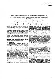
Fig. 1. Model of WP-MLP
Fig. 1 shows the WP-MLP used in this paper. It consists of three stages, i.e., input with a tapped delay line, wavelet packet decomposition, and an MLP. The output xˆ ( n + 1) is the value of the time series at time n+1 and is a function of the values of the time series at previous time steps: s n = [ x ( n ), x ( n − 1 ), K , x ( n − p )] T
(1)
Coifman, Meyer and Wickerhauser [9] introduced wavelet packets by relating multiresolution approximations with wavelets. Recursive splitting of vector spaces is represented by a binary tree. We employed the wavelet packet transformation to produce time-frequency atoms. These atoms provide us with both time and frequency information with varying resolution through out the time-frequency plane. The timefrequency atoms can be expanded in a tree-like structure to create arbitrary titling, which is useful for signals with complex structure. A tree algorithm [10] can be employed for computing wavelet packet transform by using the wavelet coefficients as filter coefficients. The next sample is predicted using a conventional MLP with k input units, one hidden layer with m sigmoid neurons and one linear output neuron, as
312
K.K. Teo, L. Wang, and Z. Lin
shown in Fig. 1. The architecture of the WP-MLP is defined as, [ p : l ( w let ) : h ] where p is the number of tapped delays, l is the number of decomposition level, wlet is the type of wavelet packet used, and h is the number of hidden neurons. In the present work, the MLP is trained by the backpropagation algorithm using the Levenberg-Marquadt method [11].
3 Weight Initialization by Clustering Algorithms The initialization of the weights and biases has a great impact on the network training time and generalization performance. Usually, the weights and biases are initialized with small random values. If the random initial weights happen to be far from a good solution or they are near a poor local optimum, training may take a long time or get trap in the local optimum [8]. Proper weights initialization will place the weights close to a good solution, which reduces training time and increases the possibility of reaching a good solution. In this section, we describe the method of weights initialization by clustering algorithms. The time-frequency event matrix is defined by combining the time-frequency patterns and its respective targeted outputs of the training data. Each column is made up of time-frequency pattern and its respective target that is used for the clustering algorithm. The clustering analysis [13] is the organization of a collection of patterns into clusters based on similarity. In this way, the natural grouping of the timefrequency events is revealed. Member event within a valid cluster are more similar to each other than they are to an event belonging to a different cluster. The number of clusters is then chosen to be the number of neurons in the hidden layer of the WPMLP. The number of clusters may be chosen before clustering, or may be determined by the clustering algorithm. In the present work, the hierarchical clustering algorithm [14] and the counterpropagation network [15] are tested. Hierarchical clustering algorithm consist of three simple steps:
Compute the Euclidean distance between every pair of events in the data set. Group the events into a binary, hierarchical cluster tree by linking together pairs of events that are in close proximity. As the events are paired into binary clusters, the newly formed clusters are grouped into larger cluster until a hierarchical tree is formed. Cut the hierarchical tree to form the clusters according to the number of hidden neurons chosen based on a prior knowledge acquired.
Counterpropagation network is a combination of a competitive layer and another layer employing Grossberg learning. For the purpose for this paper, the forward-only variant of the counterpropagation network shall be used. Let us consider a competitive learning network consisting of a layer of Nn competitive neurons and a layer of N+1 input nodes, N being the dimension of the input pattern. hk =
N +1
∑ j
g kj x j
(2)
Wavelet Packet Multi-layer Perceptron
313
where gkj is the weight connecting k neuron to all the inputs, hk is the total input into neuron k and xj is j element of the input pattern. If neuron k has the largest total input, it will win the competition and becoming the sole neuron to response to the input pattern. The input patterns that win the competition in the same neuron are considered to be in the same cluster. The neuron that win the competition will have it weight adjust according with the equation shows below.
wkjnew = (1 − α (t )) wkjold + α (t ) x j
(3)
where learning constant α (t ) is a function of time. The other neurons do not adjust their weights. Learning constant will change according to (13) to ensure that each training pattern has equal statistical importance and independence of presentation order [16] [17].
α (τ k ) =
α (1) 1 + (τ k − 1)α (1)
(4)
where τ k ≥ 1 is the number of times neuron k has modified its weights including the current update. At the end of the training, those neurons that never had it weights modified are discarded. In this way, we had found the number of clusters and the number of hidden neurons of the WP-MLP. Both clustering algorithms had formed clusters and we can proceed to initialize the WP-MLP. The weights of the hidden neuron are assigned to be the centroid of each cluster.
4 Simulation Results We have chosen two time series often found in the literature as a benchmark, i.e., the Mackey-Glass delay-differential equation and the yearly sunspot reading. For both data sets are divided into three sections for training, validation and testing. When there is an increase in the validation error, training stops. In order to have a fair comparison, simulation is carried out for each network over 100 trials (weight initialization can be different from trial to trial, since the clustering result can depend on the random initial starting point for a cluster). 4.1 Mackey-Glass Chaotic Time Series The Mackey-Glass time-delay differential equation is defined by
dx ( t ) ax ( t − τ ) = − bx ( t ) dt 1 + x ( t − τ ) 10
(5)
where x(t) represents the concentration of blood at time t when the blood is produced. In patients with different pathologies, such as leukemia, the delay time t may become very large, and the concentration of blood will oscillate, becoming chaotic when τ ≥ 17. In order to test the learning ability of our algorithm, we choose the valuet=17 so that the time series is chaotic. The values of a and b are chosen 0.2 and 0.1
314
K.K. Teo, L. Wang, and Z. Lin
respectively. The training data sequences are of length 400, followed by validation and testing data sequences of length 100 and 500 respectively. Tests were performed on random initialization, hierarchical clustering algorithm and counterpropagation network on varying network architecture. Eight neurons in the hidden layer are chosen and this is a prior knowledge required by hierarchical clustering algorithm to cut the tree i.e. there are eight clusters. The counterpropagation network is given ten neurons to process the data to search for the optimal clustering. Table 1. Validation and test MSE of WP-MLP with random initialization on Mackey-Glass chaotic time series Validation MSE
Network Architecture
Test MSE
Mean
Std
Min
Mean
Std
Min
[14:1(Db2): 8]
4.17x10⁻⁴
1.89x10⁻⁴
2.36x10⁻⁴
1.80x10⁻⁵
8.13x10⁻⁶
1.02x10⁻⁵
[14:2(Db2): 8]
7.86 x10⁻⁵
3.71 x10⁻⁴
2.94x10⁻⁵
3.73 x10⁻⁶
1.86 x10⁻⁵
1.25 x10⁻⁶
[14:3(Db2): 8]
3.62x10
-4
-4
-4
-5
-6
9.65x10-6
*[14: 3(Db2):8]
1.15 x10⁻⁶
3.83 x10⁻⁶
1.49 x10⁻⁶
3.62x10
2.24x10
2.94 x10⁻⁶
1.56x10
1.15 x10⁻⁶
4.51x10
1.12 x10⁻⁵
*Wavelet Decomposition
Table 2. Validation and test MSE of WP-MLP initialized with hierarchical clustering algorithm on Mackey-Glass chaotic time series Validation MSE
Network Architecture
Test MSE
Mean
Std
Min.
Mean
Std
Min.
[14: 1(Db2): 8]
5.66x10⁻⁶
1.42x10⁻⁵
2.16x10⁻⁶
5.65x10⁻⁶
1.42x10⁻⁵
2.16x10⁻⁶
[14:2(Db2): 8]
2.74x10⁻⁶
2.16x10⁻⁷
2.31x10⁻⁶
2.75x10⁻⁶
3.24x10⁻⁷
2.31x10⁻⁶
[14:3(Db2): 8]
3.46x10
-6
-6
-6
-6
-6
1.53x10-6
*[14: 3(Db2):8]
2.45x10⁻⁵
5.54x10⁻⁵
1.38x10⁻⁵
1.50x10
1.53x10
5.54x10⁻⁵
3.45x10
9.06x10⁻⁶
1.65x10
2.81x10⁻⁵
*Wavelet Decomposition
Table 3. Validation and test MSE of WP-MLP initialized with counterpropagation clustering algorithm on Mackey-Glass chaotic time series Validation MSE
Network Architecture
Test MSE
Mean
Std
Min.
Mean
Std
Min.
[14: 1(Db2):10]
1.935x10⁻⁵
3.69x10⁻⁵
1.78x10⁻⁷
2.33 x10⁻⁵
4.30 x10⁻⁵
3.54 x10⁻⁷
[14:2(Db2):10]
1.02 x10⁻⁵
1.06 x10⁻⁵
1.73 x10⁻⁷
1.22 x10⁻⁵
1.21 x10⁻⁵
2.42 x10⁻⁷
[14:3(Db2):10]
2.303x10⁻⁵
4.21 x10⁻⁵
4.62 x10⁻⁷
2.96x10⁻⁵
3.52 x10⁻⁵
9.82 x10⁻⁷
-5
-5
-6
-5
-5
7.86x10-6
*[14: 3(Db2):10]
1.96 x10
1.95 x10
6.20 x10
2.34 x10
2.24 x10
*Wavelet Decomposition
Table 1 shows the results on prediction errors for the Mackey-Glass time series using different architecture of the WP-MLP, i.e. the mean, the standard deviation, and the minimum Mean Squared Error (MSE) of the prediction errors over 100 simulations. Table 2 and 3 show the result on prediction error for network initialized by hierarchical and counterpropagation respectively.
Wavelet Packet Multi-layer Perceptron
315
Hierarchical clustering algorithm provides consistent performance for the various network architecture except the network with wavelet decomposition. Counterpropagation network managed to attain the lowest minimum MSE with various network architecture. Thus we can say that it had indeed found the best clustering to place the weights near the optimum solution. The higher mean, larger standard deviation and lower minimum suggested that the probability of getting the optimal clustering is low. Therefore, the counterpropagation network needs more tuning to find the optimal clustering frequently. 4.2 Sunspots Time Series Sunspots are large blotches on the sun that is often larger in diameter than the earth. The yearly average of sunspot areas has been recorded since 1700. The sunspots of years 1700 to 1920 are chosen to be the training set, 1921 to 1955 as the validation set, while the test set is taken from 1956 to 1979. Tests were performed on random initialization, hierarchical clustering algorithm and counterpropagation network on varying network architecture. Eight neurons in the hidden layer are chosen and this is a prior knowledge required by hierarchical clustering algorithm to cut the tree i.e. there are eight clusters. The counterpropagation network is given ten neurons to process the data to search for the optimal clustering. Table 4. Validation and test NMSE of WP-MLP with random initialization on Sunspots time series Validation NMSE
Network
Test NMSE
Architecture
Mean
Std
Min
Mean
Std
Min
[12: 2(Db1): 8]
0.0879
0.300
0.0486
0.3831
0.2643
0.1249
[12:1(Db2):8]
0.0876
0.0182
0.059
0.4599
0.7785
0.1256
[12:2(Db2):8]
0.0876
0.0190
0.0515
1.0586
6.2196
0.1708
*[12:3(Db2):8]
0.0876
0.0182
0.0590
0.5063
1.0504
0.1303
*Wavelet Decomposition
Table 5. Valdiation and test NMSE of WP-MLP with initialized with hierarchical clustering algorithm on Sunspots time series Validation NMSE
Network Architecture
Mean
Std
Test NMSE Min
Mean
Std
Min
[12: 2(Db1): 8]
0.0674
0.0123
0.0516
0.2682
0.1716
0.1305
[12:1(Db2):8]
0.0714
0.0103
0.0499
0.2906
0.1942
0.1426
[12:2(Db2):8]
0.0629
0.0100
0.0508
0.2126
0.0624
0.1565
*[12:3(Db2):8]
0.0691
0.0069
0.0523
0.2147
0.0585
0.1430
*Wavelet Decomposition
316
K.K. Teo, L. Wang, and Z. Lin
Table 6. Validation and test NMSE of WP-MLP with counterpropagation clustering algorithm on Sunspots time series Validation NMSE
Network Architecture
Test NMSE
Mean
Std
Min
Mean
Std
Min
[12: 2(Db1): 10]
0.079
0.0121
0.050
0.277
0.0819
0.1383
[12:1(Db2):10]
0.078
0.012
0.047
0.271
0.0880
0.1451
[12:2(Db2):10]
0.078
0.0130
0.0485
0.2722
0.0722
0.1442
*[12:3(Db2):10]
0.071
0.011
0.048
0.252
0.0631
0.1324
*Wavelet Decomposition
Table 5 shows the results on prediction errors for the Sunspot time series using different architecture of the WP-MLP, i.e. the mean, the standard deviation, and the minimum Normalized Mean Squared Error (NMSE) of the prediction errors over 100 simulations. Table 6 and 7 show the result on prediction error for network initialized by hierarchical and counterpropagation respectively. Both initialization methods shown superior performance in all aspect compared to the WP-MLP that is initialized randomly. Thus we can say that for the problem of sunspots, the initialization methods place the weights close to a good solution frequently.
5 Conclusion In this paper, we used hierarchical and counterpropagation clustering algorithms to initialize WP-MLP for time series prediction. Usually the weights are initialized with small random values that maybe far from or close to a good solution. Therefore the probability of being located near a good solution depends on the complexity of the solution space. In a relatively simpler problem such as Mackey-Glass time series, it is expected to have less poor local optimum. Thus the chance of being placed near a good solution is higher and initialization of weights may not be important. When dealing with difficult problem like Sunspot time series, it is expected to have a complex solution space that has lot of local optima. Thus random initialization cannot provide the consistent performance attained by the both initialization methods. Therefore, the weights of the WP-MLP must be initialized to achieve better performance.
REFERENCE 1. 2. 3.
Lapedes, A., Farber, R.: Nonlinear Signal Processing Using Neural Network: Prediction and System Modeling. Los Alamos Nat. Lab Tech. Rep, LA-UR-872662 (1987) Mallat, S.G.: Multifrequency channel decompositions of images and wavelet models. IEEE Transactions on Acoustics, Speech and Signal Processing, Vol. 37, No. 12 (1989) 2091 – 2110 Mallat, S.G.: A Theory for Multiresolution Signal Decomposition: The Wavelet Representation. IEEE Transactions on Pattern Recognition, Vol. 11, No. 7 (1989) 674 – 693
Wavelet Packet Multi-layer Perceptron 4. 5. 6. 7. 8. 9. 10. 11. 12. 13. 14. 15. 16. 17. 18. 19.
317
Vetterli, M., Herley, C.: Wavelets and filter banks: theory and design. IEEE Transactions on Signal Processing, Vol. 40, No.9 (1992) 2207 –2232 Mallat, S.G.: A Wavelet Tour of Signal Processing. Academic Press (1998) Strang, G., Nguyen, T.: Wavelet and Filter Banks. Wellesly-Cambridge Press (1996) Zhang, Q., Benveniste, A.: Wavelet Networks. IEEE Transactions on Neural Networks, Vol. 3, No. 6. (1992) 889 -898 Kolen, J.F., Pollack, J.B.: Back Propagation is Sensitive to Initial Conditions. Tech. Rep. TR 90-JK-BPSIC, Laboratory for Artifical Intelligence Research, Computer and Information Science Department, (1990) Coifman, R.R., Meyer, Y., Wickerhauser, M.V.: Entropy-Based Algorithm for Best Basis Selection. IEEE Transactions on Information Theory, Vol. 38, No. 2 Part 2 (1992) 713-718 Vetterli, M., Herley, C.: Wavelets and filter banks: theory and design. IEEE Transactions on Signal Processing, Vol. 40, No.9 (1992) 2207–2232 Hagan, M.T., Menhaj, M.B.: Training Feedforward Networks with the Marquardt Algorithm. IEEE Transactions on Neural Networks, Vol. 5, No. 6 (1994) 989 -993 Geva, A.B.: ScaleNet-Multiscale Neural-Network Architecture for Time Series Prediction. IEEE Transactions on Neural Networks, Vol. 9, No. 9 (1998) 1471 –1482 Jain, A.K., Murty, M.N., Flynn, P.J.: Data Clustering: A Review. ACM Computing Surveys, Vol. 31, No. 3 (1999) 264-323 Aldenderfer, M.S., Blashfield, R.K.: Cluster Analysis. Sage Publications (1984) Nielsen, R.H.: Neurocomputing. Addisson-Wesley Publishing Company. (1990) Wang, L.: On competitive learning. IEEE Transaction on Neural Network, Vol. 8,No. 5 (1997) 1214-1217 Wang, L.: Oscillatory and Chaotic dynamic in neural networks under varying operating conditions. IEEE Transactions on Neural Network, Vol. 7, No. 6 (1996) 1382-1388 Denoeux, T., Lengelle, R.: Initializing back propagation network with prototypes. Neural Computation, Vol. 6 (1993) 351-363 Lehtokangas, M., Saarinen, J., Kaski, K., Huuhtanen, P.: Initialization weights of a multiplayer perceptron by using the orthogonal least squares algorithm. Neural Comput., Vol. 7, (1995) 982-999