J. Phys. A: Math. Gen. 29 (1996) 2509–2527. Printed in the UK
Wavelet packet computation of the Hurst exponent C L Jones†§k, G T Lonergan† and D E Mainwaring‡ † Centre for Applied Colloid and BioColloid Science, School of Chemical Sciences, Swinburne University of Technology, Hawthorn 3122, Australia ‡ Department of Applied Chemistry, Royal Melbourne Institute of Technology, Melbourne 3001, Australia
Received 11 July 1995, in final form 27 November 1995
Abstract. Wavelet packet analysis was used to measure the global scaling behaviour of homogeneous fractal signals from the slope of decay for discrete wavelet coefficients belonging to the adapted wavelet best basis. A new scaling function for the size distribution correlation between wavelet coefficient energy magnitude and position in a sorted vector listing is described in terms of a power law to estimate the Hurst exponent. Profile irregularity and long-range correlations in self-affine systems can be identified and indexed with the Hurst exponent, and synthetic one-dimensional fractional Brownian motion (fBm) type profiles are used to illustrate and test the proposed wavelet packet expansion. We also demonstrate an initial application to a biological problem concerning the spatial distribution of local enzyme concentration in fungal colonies which can be modelled as a self-affine trace or an ‘enzyme walk’. The robustness of the wavelet approach applied to this stochastic system is presented, and comparison is made between the wavelet packet method and the root-mean-square roughness and second-moment approaches for both examples. The wavelet packet method to estimate the global Hurst exponent appears to have similar accuracy compared with other methods, but its main advantage is the extensive choice of available analysing wavelet filter functions for characterizing periodic and oscillatory signals.
1. Introduction The wavelet transform is a mathematical technique which is useful for numerical analysis and manipulation of both one- and two-dimensional signal sets. The transform operates like a microscope for detail examination by partitioning the signal into different frequency components mapped to coefficients having different energies [1]. The wavelet decomposition therefore provides information about how energy depends on position and scale. The resolution scale can be changed to focus on local features by applying a set of specially constructed ‘filters’ which transform (dilate and translate) the input signal in an iterative scheme. This approach is not unlike traditional Fourier series expansions of functions using sines, cosines or exponentials, although a linear combination of wavelet functions is used to represent the signal function f (i). Wavelets attempt to avoid inherent difficulties with the spectral approach such as lack of convergence, and offer a class of flexible functions with prescribed smoothness that are well localized with respect to position and frequency. § Author to whom correspondence should be addressed. k E-mail address:
[email protected] c 1996 IOP Publishing Ltd 0305-4470/96/102509+19$19.50
2509
2510
C L Jones et al
Previously, the wavelet transform has been used for the characterization of fractal [2] and multifractal signals [3, 4], turbulence data [5], branching of diffusion-limited aggregates [6, 7] and spatiotemporal time series analysis [8]. This paper presents a new scaling relation to derive the global Hurst ‘roughness’ exponent from the slope of decay for the size distribution of coefficient energies calculated from wavelet packet analysis, WPA [9– 11]. It should be emphasized that the wavelet transform is thought to provide a statistical– mechanical description [7] of the construction process for feature-to-coefficient mapping into the best basis which represents the collective mapping with lowest information cost [12]. Here we compare WPA with several alternative measurement methods for characterizing global statistical properties of 1D self-affine signal profiles. The organization of this paper is as follows. Section 1.1 defines the scope of this investigation while section 1.2 reviews the importance of the homogeneous global selfaffine exponent. Section 2 presents the biological background and rationale for applying WPA to examine spatially non-uniform enzyme patterns in biological systems. Section 3 details the mechanics of applying WPA to characterize self-affine signals. Section 4 details how to practically expand synthetic and stochastic self-affine signals to quantify the Hurst exponent. Section 5 defines the power-law behaviour for the wavelet packet best basis, while section 6 reviews the issue of finite-size effects which impact on the accurate description of short signals. The results for WPA compared against three alternative methods are presented and discussed in sections 7 and 8. The methods for enzyme detection and fungal growth are provided in appendix A. 1.1. Scope of the investigation The accuracy and reliability of four different methods to characterize the profile irregularity of short 1D signals was examined by testing each method against synthetic self-affine profiles which have a prescribed Hurst exponent. We do not consider multifractal signals, nor do we examine ‘local’ scaling properties at intermediate length scales. The purpose of this paper is to introduce WPA as an additional method to quantify the homogeneous or global ‘monofractal’ [13] behaviour of self-affine 1D signals by estimating the Hurst roughness exponent. We comment briefly in the discussion on another multifractal approach, in particular, the wavelet transform modulus-maxima (e.g. [4, 5]) and how the WPA method presented here could be improved to estimate local scaling trends. Details for calculating the local H exponent to estimate possible multifractal behaviour of self-affine 1D signals using WPA is given in appendix B. We also demonstrate the potential of this technique by quantifying the self-affine irregularity of gray-scale elevation line profiles which had been extracted from digital images of spatially distributed data. We point out that all stochastic 1D signals examined here were obtained from 2D images captured using image analysis, and the synthetic fBm-type profiles were of length L = 512. Short signals where L 6 512 were chosen in order to more closely mimic those which can be experimentally extracted using image analysis (i.e. with a 512 × 512 pixel resolution framegrabber and CCD camera). We briefly review other studies which have investigated the self-affine properties of short signals (L < 1024) in section 6. 1.2. Importance of the self-affine exponent Statistical properties of selected one-dimensional profiles were examined to characterize how the point-to-point signal distribution scales and fills the available space. Self-affine fractal objects are invariant under an affine transformation [14]. The stochastic surface
Wavelet packet computation of the Hurst exponent
2511
roughness was investigated with line profiles extracted from the 2D plane where the x and y locations are positionally defined but the vertical axis (or z-plane elevation) was a fluctuating quantity. Magnified portions of such signals do not scale equally in all directions (x, y and z) resulting in scalar anisotropy. This violates the property of true self-similarity where finer feature details, under a magnification scale transform, should occur isotropically in all directions. The magnification factor used to rescale self-affine functions therefore depends on the direction. Sample profiles of fractional Brownian motion (fBm) are often used to illustrate statistical scaling properties of random walks. A fBm, VH (i) models the scaling of a single variable, i used here to index position. The Hurst exponent, H measures the fluctuation for the increments of fBm, 1i which are derived by considering the scaling function 1VH (1i) = VH (i2 ) − VH (i1 ). This has a Gaussian distribution with variance [15] averaged over many realizations of VH (i): h1VH (1i)i ∝ 1i 2H .
(1)
In one dimension, it has been shown [15] that equation (1) is equivalent to examining how the average width or height difference 1h(x) of the function VH (i) scales according to H over different linear subregions of length x: 1h(x) ∼ x H .
(2)
An obvious property which can be examined for each fBm-type profile walk sequence is the degree of correlation between adjacent regions. Since H ∈ (0, 1) and 0 < H < 1, three types of behaviour can be identified. Short-range antipersistent correlations (H < 0.5) are typically characterized by peaks followed by troughs in an alternate sequence; random fluctuations (white noise H = 12 ) are uncorrelated, while long-range correlations (H > 0.5) are persistent and display some form of ‘memory’. 2. Biological background We examine several numerical methods which estimate the global Hurst exponent to index the nearest neighbour statistical distribution of enzyme concentration in spatially extended fungal colonies. Details of colony growth and enzyme detection are given in appendix A. Fungal colonies develop from locally interacting cell systems which express exo-enzymes, such as laccase to break down substrate constituents. Exo-enzyme secretion is known to occur principally via the hyphal tips, and different substrate compositions (concentration of the carbon source, or the presence of paramorphogens which influence branching) induce the formation of macroscopic patterns of enzyme activity with very different spatial scales. For example compare figure 1(b) with 1(h). These are examples of a reacting chemical system [16] where signal transmission from the extracellular environment effects intracellular biochemical events. Diffusive transport in turn gives rise to macroscopic aggregating bands of enzyme activity (figure 1(e) and 1(h)). This study therefore introduces a possible experimental approach to the question of morphogenetic regulation of cell growth and differentiation and how this is related to biochemical synthesizing systems and their spatial organization. This biological example belongs to a class of more general chemical feedback problems which generate spatial patterns via chemical diffusion, oscillations, travelling waves or multistability [16, 17]. The WPA method is used here to characterize correlation properties in the spatial ordering of biochemical concentration, visualized as one-dimensional fBm-type profiles, termed ‘enzyme walks’ in these biological systems. The WPA method extends the experimental
2512
C L Jones et al
Figure 1. (a) Photograph of a single colony of Pycnoporus cinnabarinus grown from a single spore on malt extract agar at 37 ◦ C for 22 hours; scale: bar ≡ 100 µm. (b) Colony of P. cinnabarinus at day 3 grown from a central plug inoculum containing many spores. Orange stain indicates laccase enzyme detected with 2, 6-dimethoxyphenol reagent after 120 min; membrane diameter = 47 mm. (c) Single digital line profile extracted from edge to edge across the whole colony—ALL; membrane diameter = 47 mm. (d ) Single digital line profile extracted from the centre-point to the edge—HALF. Scale bar = 5 mm. (e) Pseudo-colour representation of (b) and (c) showing the double-banding pattern characteristic of laccase enzyme expression in this fungus. The arrow indicates the centre-point inoculum, growth is radially symmetric outwards from here over time; scale bar = 10 mm. (f ) Enlarged view of a single line profile indicating gray-scale amplitude (intensity signal) fluctuation for ALL; scale bar = 10 mm. (g) Gray-scale amplitude fluctuation for a single line extracted from HALF; scale bar = 5 mm. (h) The influence of nutrient substrate concentration on the double band pattern of laccase enzyme at day 3 for P. cinnabarinus grown on ground wood (0.2%) + agar(2%) + 1000 ppm of the industrial dye, Remazol Brilliant Blue R. Note the spatial delineation of banding into two discrete regions and compare with (b). This image was recorded 120 minutes after reagent addition. Membrane diameter = 47 mm.
techniques previously used to detail the acid phosphatase enzyme system [18, 19]. Here, deposition of the reagent, 2, 6-dimethoxyphenol [20] was used to reveal sites of the extracellular enzyme, laccase (benzenediol:oxygen oxidoreductase, E.C.1.10.3.2)—which
Wavelet packet computation of the Hurst exponent
2513
formed a rough interface with distinct concentration regions of enzyme activity. We analyse the pattern of spatial distribution of laccase concentration, and measure its roughness exponent, H using all four methods. Self-affine biosequences for acid phosphatase had previously been analysed by an alternative scaling method (fast Fourier transform [18]) to empirically describe cellular information processing with respect to enzymatic complexity and percolation threshold phenomena [19] occurring in biochemical systems. Digital line profiles were extracted using computerized image analysis to investigate macroscopic biological pattern formations which develop from in vivo enzyme expression of whole fungal colonies [18, 19]. Colony growth is radially symmetric outwards from a central plug inoculum, and occurs by repeated branching of vegetative filaments called hyphae shown in figure 1(a). The structural development of morphology during early colony growth is very similar in appearance to the off-lattice Eden cluster growth network [21]. In many fungi, laccase enzyme is involved with catabolic degradation for active maintenance of nutrition [22]. Typically, a series of linear line profile functions are obtained f (z)i , i = 1, 2, . . . , L, which can be described with a dual coordinate system indexing position i of length L along the x-axis versus enzyme concentration measured as gray-scale intensity amplitude (z-axis) in hue, saturation, intensity (HSI) colour signal space. The global quantitative description of the irregularity (or ‘jaggedness’) observed in these profiles was solved by estimating the self-affine fractal dimension with the Hurst exponent [18], and is similar to the numerical methods used to quantify ‘DNA walks’ [23] and heartbeat interval fluctuations [24]. This experimental approach to describe scale invariance in spatially extended systems has popularly been termed a ‘statistical–mechanical approach’ [24], in that micro-level scaling correlations are thought to impact on macro-level structural patterns. This viewpoint shares common features with adaptive walk models on fitness landscapes [25, 19] and the emergence of self-organized criticality [26] to explain a possible mechanism underlying such patterns of fluctuation activity. 3. Wavelet packet transform analysis 3.1. Mechanics of applying wavelet packet transform to self-affine signals The wavelet transform partitions a signal with respect to spatial frequency [10]. This is achieved by filtering the signal with a pair of dyadic orthogonal filters termed a quadrature mirror filter (QMF) which operates according to sub-band coding [27]. This is a multiresolution scheme [10, 28] which separates the signal into coarse and fine-multiresolution components using a low-pass filter to obtain successively blurred versions of the input signal, and a high-pass filter to select the high-frequency component. Figure 2 illustrates the ‘pairfamily’ concept of wavelet filter functions. For the Haar (d2) wavelet, the low-pass filter, often notationally defined as the ‘father’ wavelet φ is the scaling function and integrates to one, while the ‘mother’ wavelet 9 integrates to zero. Other filter properties for higher-order wavelets are given in the figure caption. Linear combinations of wavelet functions which oscillate about zero can then be used to represent or approximate 1D signals. Wavelets are especially useful for examining signals which have sharp jumps and which are more difficult to resolve using Fourier series approximation methods. Four orthogonal wavelet filter functions are shown in figure 2 which differ in their degree of oscillation and regularity. We explore the impact that different filter architectures have on achieving successful signal approximation, and how this relates to ‘smoothness’ detection in our goal to estimate the global Hurst exponent. The Haar wavelet (d2) is a square wave with compact support and is symmetric; however, it is not continuous and has poor position–frequency localization [1].
2514
C L Jones et al
Figure 2. Some examples of orthonormal wavelet bases. For each ‘mother’ filter 9 the family 9m,n (i) = 2−m/2 9b (2−m i − n) provides an orthonormal basis. This figure plots the associated ‘father’ φ scaling function for each 9; left: father wavelets; right: mother wavelets. The Haar wavelet has support length = 1, no vanishing moments, and H¨older exponent = 0. The d4 wavelet has support length = 3, 1 vanishing moment for 9 and a H¨older exponent = 0.55. The d6 wavelet has support length = 5, 2 vanishing moments for 9 and a H¨older exponent = 1.09. The d8 wavelet has support length = 7, 3 vanishing moments for 9 and a H¨older exponent = 1.62. Smooth wavelets have wide support and a higher number of vanishing moments allowing the wavelet better representation of higher-degree polynomial signals. The H¨older exponent is another measure of smoothness.
Notably different wavelet packet functions Wb (i) are generated by scaling and translating one of the QMF filters. Each function has a frequency b which describes the number of oscillations or zero crossings the wavelet packet makes. For the Haar basis, the wavelet does not oscillate through zero (b = 0) so φ(i) ≡ W0 (i) but the mother wavelet has one zero crossing (b = 1) so 9(i) ≡ W1 (i). WPA operates by approximating a signal with scaled and translated wavelet packet functions Wm,b,n which are generated from Wb following: Wm,b,n (i) = 2−m/2 Wb (2−m i − n) .
(3)
The notation which characterizes each wavelet packet Wm,b,n reflects the scale 2m and location 2m n. The resolution level changes with m and the translation operates through n. A signal f (i) can then be represented by the sum of orthogonal wavelet packet functions Wm,b,n (i) following XXX wm,b,n Wm,b,n (i) . (4) f (i) ≈ m
b
n
The wavelet packet coefficients (in final form identified with the notation Cnm ) are produced
Wavelet packet computation of the Hurst exponent from this integral: Cnm
2515
Z ≡ wm,b,n ≈
Wm,b,n (i)f (i) di .
(5)
It should be emphasized that equation (4) allows many possible combinations of wavelet packet functions to be selected in order to optimally characterize the signal. This contrasts with the more general wavelet transform (DWT) [29–32] used to analyse fractal signals where the wavelet functions are fixed at discrete resolution levels. 3.2. The wavelet packet transform and adapted waveform analysis for 1D signals The objective of WPA is to create a binary tree decomposition of the signal into a set of energy levels, called ‘octave’ windows [9] where the frequency domain has been divided logarithmically [33]. During the segmentation, each scale retains the dominant signal features while minimizing the wavelet coefficient amplitude of their representation. Because the wavelet packet coefficients contain information about the energy magnitude contribution for each discrete feature in terms of scale, frequency and position, this provides a robust method for feature and singularity detection. It is notable that determination of the singularity spectrum of fractal functions by wavelet analysis provides a microscopic statistical description of the scaling behaviour in terms of thermodynamic energy functions [7]. Convolving the signal (subsampling) at each iteration by keeping only every second point makes the expansion into the wavelet packet best basis finite [10, 34]. Each transformation into the next level is an energy conservation process, and the total energy is considered to be the sum of all the individual energies mapping out the feature fluctuations. The input signal can also be rebuilt via upsampling and summing combinations of coefficients. By choosing a set of mother and father wavelet functions (a QMF) with known oscillation index, one can decompose an input signal to create a wavelet packet table. Figure 3 shows the wavelet packet table created using the d4 wavelet function for an input fBmtype signal with L = 512 and theoretical H = 0.2 which had been created with the midpoint displacement method [35]. Each resolution level, m has 512 coefficients and is subdivided into blocks which contain the wavelet packet coefficients with an oscillation index b = 0, 1, . . . 2m − 1. Level 0 reproduces the input, and resolution levels 1 to 8 are plotted in descending order. For each level, the leftmost block corresponds to an oscillation index b = 0 and contains the low-frequency approximation coefficients. The rightmost block (or blocks) have an oscillation index b = 2m − 1 and contain the high-frequency, detail coefficients. Notably, the wavelet packet table is a redundant approximation of the signal and for an input signal of L = 512 the table contains (M + 1) × 512 coefficients. For a signal of L = 512, M is equivalent to the total number of resolution scales, m—which in this case is eight. We can now select a subset of coefficients from the wavelet packet table to create a unique, orthogonal wavelet packet transform. To select an optimal transform of bases from the wavelet packet table, the best basis algorithm of Coifman and Wickerhauser [12] was used. This algorithm is adaptive in that it minimizes a cost function by finding the minimum entropy for coefficients [10] which belong to the best basis. To emphasize the superiority of the wavelet packet transform (WPT) best basis method which is fundamental to WPA for signal approximation compared with the more common discrete wavelet transform (DWT), we decompose the input signal used in figure 3 with the d4 wavelet (figure 4). On the left, the DWT provides good decomposition of the coarse signal features but the WPT on the right results in superior decomposition and localization of fine, detail signal features. For the DWT, each detail resolution level
2516
C L Jones et al
Figure 3. Wavelet packet table for a sample fBm-type 1D signal with H = 0.2 and L = 512, created by midpoint displacement. The QMF filter was the d4 wavelet. Level 0 is equivalent to the original signal and resolution level 1 through 8 are plotted below. For each level, the leftmost block has oscillation index b = 0 and is the ‘approximation’ or blurred signal created from the low-pass father φ wavelet which convolves the signal by keeping only every second point. The rightmost block has oscillation index b = 2m − 1 and contains the high-frequency coefficients created from the high-pass 9 mother wavelet. The wavelet packet coefficients wm,b,n are plotted as a fluctuating vertical line in the rightmost blocks. Coefficient index position extends from 0 to 512 for level 0 on the x-axis.
Figure 4. Comparison of wavelet decomposition with wavelet packet decomposition for a fBmtype signal with H = 0.2; left: discrete wavelet transform decomposition (DWT); right: best basis wavelet packet decomposition (WPA) with the d4 wavelet. The DWT identifies the coarse features but the wavelet packet transform with the best basis coefficients provides a more refined decomposition of the high-frequency, fine-scale features.
Wavelet packet computation of the Hurst exponent
2517
is indexed by D and the smooth signal by S. The greater number of best basis function blocks for the best basis decomposition results in superior detection of local scaling trends. We then combine these coefficients into a single listing, and estimate the power-law decay of sorted coefficient energies to determine the homogeneous Hurst exponent (following the protocol described in section 4.1 and section 5). 4. Computation of the global Hurst exponent using
WPA
4.1. Application to short synthetic 1D profiles Synthetic fBm-type, one-dimensional profiles were created at L = 512 pixel length using the midpoint displacement algorithm [35]. The method of wavelet packet analysis [9–11], was used for wavelet analysis of fifteen test profiles each with predicted H = 0.3, 0.5 and 0.7, respectively. An example profile for H = 0.3 is shown in figure 5(a). In addition, H was estimated using the root-mean-square roughness (RMS versus L) method [35] and growth of the second moment, and growth of the local second moment [36]. The Daubechies two (Haar), four, six and eight (d2–d8) compactly supported wavelet functions [9] shown in figure 2 were used to expand the source signal into a binary tree consisting of multiple resolution levels. These filters were also applied to fifteen ‘enzyme walk’ profiles at two magnifications to assess the utility of higher-order wavelet functions on accuracy. Each successive level of the expansion represents the signal using a greater number of nodes but a decreasing number of coefficients. The best basis was selected for reconstruction using the Shannon entropy criterion [9–11]. Reconstruction in this way encodes most of the important signal information onto the coherent subset and leaves the degenerate portion of the signal
Figure 5. Wavelet-based analysis of a sample fBm-type profile (L = 512). Graph of deterministic function with (a) H = 0.3; RMS versus L, H = 0.409 ± 0.014; H (second moment) = 0.261, r 2 = 0.954; H (local second moment) = 0.330. (b) Wavelet basis powerlaw spectrum of Nr (Cnm > N ) versus N computed with the d6 wavelet filter, the slope of line δ = −1.325, r 2 = 0.786; predicted H = 0.325. Finite-size effects contribute to the deviation from linearity, producing a ‘tail’ for the distribution, however these coefficients are not rejected since they contribute non-negligible energy magnitude (E > 0) to the size distribution.
2518
C L Jones et al
(i.e. noise) mapped onto the residual subset. The best basis wavelet coefficients were used for synthesis of the reconstructed (coherent) signal via upsampling and summing of both the approximate and detail coefficients generated from application of φ and 9, respectively. Another best basis, called the wavelet best basis can be extracted from the coherent signal and was used to derive the Hurst exponent. The wavelet best basis coefficient subset, Cnm of the reconstructed signal after expansion (dilation by a scale term m, translation by a frequency term n) [11] was retained as data vector 1 and sorted into decreasing order of magnitude: {Cnm : C1 > C2 > · · · > Ccut-off > 0} .
(6)
A second vector listing corresponding to the coefficient index position N was similarly constructed where N is the set of all positive integers: {N1 , N2 , . . . , Ncut-off } .
(7)
A log–log plot of this relationship was constructed and a least-squares linear regression was fitted to determine the slope, δ, which indexed the sequential variation in scaling amplitude. An example is shown in figure 5(a) and (b). The mathematical rationale supporting this statistical approach is discussed in section 5. This format for wavelet data correlation allows for empirical estimation of the energy decay rate which is associated with the wavelet coefficient series for the different signals and is similar in operation to a Fourier transform spectrum of 1 − f type signals [28]. 4.2. Application to short 1D ‘enzyme walk’ profiles Biosequence profiles of laccase enzyme activity were extracted with L = 256 from threeday-old surface-grown colonies of the fungus Pycnoporus cinnabarinus, using a previously developed transmitted light imaging technique [18] and enzyme detection protocol [37]. The framegrabber hardware had a spatial pixel resolution of 512 × 512 which was equivalent to a screen pixel resolution of 384 (x-axis) versus 512 (y-axis) implemented with a rectangular pixel array. Digital 1D profiles can have a maximum length of 512 or 384 depending on image orientation. Further details of the experimental method are provided in appendix A. Sample ‘enzyme walk’ profiles are shown in figure 6 in section 7. 5. Power-law scaling The observed scaling between discrete coefficient energy magnitude and position is modelled in a sorted listing using the Korcak number-size frequency distribution power law [38]. This shares a similar mathematical formalism to the Pareto distribution [39] and the Mandelbrot– Zipf generalization [40, 41], where one considers the number Nr of objects of size [A] greater than some minimum size [a] and relates this function to a frequency distribution. Rank and frequency can be introduced by making number analogous with probability [42] where the overall power law can be expressed by Nr (A > a) ∝ ka −δ
(8)
where k is a constant and δ is the slope exponent. Since we are considering a wavelet packet expansion which returns combinations of approximation and detail coefficients that minimize the entropy of their expansion (i.e. following best basis selection), this leads to a power-law relationship between number, Nr of coefficients Cnm having a particular energy size magnitude, and index position, N : Nr (Cnm > N) ∝ kN −δ ≈ kN −(1+H ) .
(9)
Wavelet packet computation of the Hurst exponent
2519
Figure 6. A single ‘enzyme walk’ biosequence fluctuation of laccase across the whole plate (ALL) for (a). The line profile (L = 256) was placed across the radially symmetric colony (from edge to edge), and passed through the origin centre-point inoculum (at position ∼130). Results for each wavelet are: d2 wavelet: H = 0.442, r 2 = 0.390; d4 wavelet: H = 0.349, r 2 = 0.813; d6 wavelet: H = 0.376, r 2 = 0.818; d8 wavelet: H = 0.356, r 2 = 0.670; RMS versus L, H = 0.423 ± 0.031; H (second moment) = 0.293, r 2 = 0.988; H (local second moment) = 0.280. (b) Frequency partitioning for the wavelet packet transform of ALL shown in (a) with the d4 wavelet. The best basis ‘entropy’ algorithm was used to compute the best basis from the wavelet packet table and these coefficient blocks are shown in black. By doubling the magnification and taking a line profile from the centre-point to the right-hand edge, sensitivity to resolution scale changes could be examined. A single ‘enzyme walk’ is shown for HALF. (c) Results for each wavelet are: d2 wavelet; H = 0.400, r 2 = 0.375; d4 wavelet: H = 0.455, r 2 = 0.510; d6 wavelet: H = 0.370, r 2 = 0.845; d8 wavelet: H = 0.350, r 2 = 0.817; RMS versus L, H = 0.350 ± 0.026; H (second moment) = 0.164, r 2 = 0.944; H (local second moment) = 0.236. (d ) Frequency partitioning for the wavelet packet transform of HALF shown in (c) with the d4 wavelet.
The Hurst exponent parameter H is bounded by 0 < H < 1 for a graph of the function with a least-squares linear regression fit through the data points. Since the slope exponent in (8) and (9) is equivalent to −(1 + H ), the Hurst exponent may be determined from the rearrangement of terms: (δ) + 1 = |H |
or
H = |(δ + 1)| .
(10)
2520
C L Jones et al
Figure 6. (Continued.)
By sorting the coefficients Cnm into decreasing order of discrete energy ε: C1 > C2 > · · · > CE > 0
(11)
one can include best basis coefficients up to a particular energy value E which is the cut-off in equations (6) and (7). Therefore all included coefficients having discrete energies ε will be greater than or equal to E. It was found that for the d2 wavelet, the cut-off for smallest E was to reject coefficients having discrete energies ε . 0.25. This was necessary when using WPA for analysis of both fBm-type profiles and the ‘enzyme walks’. For higherorder wavelet filters such as d4, d6, and d8 the cut-off E was equivalent to including all non-negative coefficient energies. 6. Finite-size effects We review a series of practical studies which have experimentally determined the Hurst exponent on relatively short signal lengths and comment briefly on these published results in the context of the WPA data presented here. It is well known that the global self-affine exponent converges towards a more stable value for long (L > 1024) 1D signals [13]. These authors emphasize that no one method provides robust estimation of H across the possible range (H ∈ 0, 1), and that generally profiles with finite length (especially L < 1024)
Wavelet packet computation of the Hurst exponent
2521
are difficult to empirically measure. However, notwithstanding this finite-size effect, if a restricted range of self-affine exponents is observed in practice then the intrinsic errors associated with a specific algorithm can be diminished by large statistical sampling and the use of multiple methods to confirm the observed H estimate [13]. In another recent experiment [32], the discrete wavelet transform using the Haar basis was applied to 256 realizations of fBm increments of L = 128. Summary data were only given for simulations using L = 512 and our results using WPA (see table 1) are in good agreement with the accuracy across the range of synthetic fBm-type profiles examined in both experiments.
Table 1. Global Hurst exponent results for each of the different methods tested against 15 synthetic fBm-type profiles and 15 stochastic ‘enzyme walks’ for laccase. Self-affine 1D profiles Theoretical H fBm-type 03
0.5
0.7
‘enzyme walk’ ALL
‘enzyme walk’ HALF Double magnification
Data are the means of 15 replicates
d2 ‘Haar basis’ wavelet
d4 wavelet
d6 wavelet
d8 wavelet
Mean Std. dev ± r2 Std. dev ± Mean Std. dev ± r2 Std. dev ± Mean Std. dev ± r2 Std.dev ± Mean Std. dev ± r2 Std. dev ± Mean Std. dev ± r2 Std. dev ±
0.245 0.066 0.784 0.067 0.418 0.094 0.836 0.027 0.645 0.048 0.888 0.020 0.362 0.081 0.498 0.169 0.354 0.108 0.466 0.200
0.290 0.062 0.812 0.056 0.486 0.070 0.861 0.030 0.746 0.066 0.905 0.027 0.375 0.063 0.728 0.117 0.367 0.082 0.666 0.176
0.319 0.060 0.786 0.045 0.525 0.034 0.840 0.042 0.717 0.048 0.895 0.029 0.370 0.066 0.777 0.060 0.345 0.081 0.768 0.044
0.268 0.058 0.765 0.052 0.516 0.066 0.820 0.036 0.675 0.065 0.886 0.026 0.362 0.064 0.768 0.054 0.332 0.074 0.772 0.013
RMS
vs L
0.315 0.044
0.443 0.026
0.652 0.051
0.406 0.017
0.367 0.041
Global 2nd moment 0.284 0.070 0.961 0.064 0.518 0.062 0.992 0.012 0.750 0.068 0.998 0.001 0.321 0.032 0.982 0.007 0.245 0.078 0.965 0.017
‘Mean’ local 2nd moment 0.297 0.072
0.516 0.063
0.710 0.090
0.275 0.017
0.257 0.040
Two relevant studies have used a series of line profiles to measure self-affine scaling properties in 2D bone x-rays using image analysis. The first [43] used the power spectrum approach on 1D lines of L = 200. The data for 1D profiles are in good agreement with those obtained by performing 2D power spectral analysis of the same test images. The second study [44] used a series of 1D lines of L = 100 to estimate the Hurst exponent of radiological images of bone density. This last study employed imaging hardware with 512 × 512 pixel resolution. It appears that provided one examines many realizations for a given image, short profiles can be experimentally characterized with a global Hurst exponent to index roughness. Notably, in a recent time series investigation, the mean-square displacement function was measured for sequences of L = 90 and 240 with apparent successful results [45]. Finally, the growth of rough surfaces with random deposition and surface diffusion was explored over various lengths, and the data suggest [46] good agreement with scaling convergence observed between L = 120 and 450.
2522
C L Jones et al
7. Results and discussion For our simulations, fifteen samples of fBm (L = 512) were created by iterated midpoint displacement for each of the following exponents: H = 0.3, H = 0.5 and H = 0.7. The RMS versus L, global second moment, local second moment and WPA algorithms were first tested on the simulated fBm signals. The resulting mean, standard deviation and coefficient of variation and corresponding standard deviation estimated by each method are given in table 1. This table also shows the estimated H exponent when the WPA algorithm was implemented with the Haar (d2) basis and then with higher-order Daubechies filters—d4, d6 and d8. For the synthetic profiles of L = 512, the Haar wavelet (d2) consistently underestimates the Hurst exponent although the application of higher-order wavelet filters which have a greater number of vanishing moments appears to increase the accuracy of the returned exponent. This is consistent with [29], although it is important to point out the following possible caveat on this. Reference [32] applied the DWT to estimate 1D fBm signals with d4 and d16 filters. It was shown that higher-order wavelet filters can be successfully applied to estimate spatial correlations. However, higher order (i.e. d16) did not always result in faster decay of coefficient energy. In fact, excessively high order often showed a variance bias by excluding fine feature details. Further work with WPA will need to address the issue of wavelet filter order on accuracy. Considering the four wavelet filters together, for increasingly smooth signals (i.e. H = 0.5 and H = 0.7) the least-squares regression line more closely follows the power-law scaling proposed in equation (9) compared with both the mean r 2 value and the corresponding standard deviation of the regression for the antipersistent H = 0.3 signal. Specifically for H = 0.3, the mean and standard deviation for the r 2 estimate of the straight line regression fit was 0.787 ± 0.055. For H = 0.5 and H = 0.7 the mean and standard deviation were 0.839 ± 0.034 and 0.894 ± 0.026, respectively. This emphasizes the underlying irregularity of antipersistent functions and the difficulty of fitting a straight line to plots of coefficient energy magnitude versus position. It should be emphasized that such low mean r 2 values are not uncommon during computation of the Hurst exponent for self-affine functions using the alternative fast Fourier transform method where a typical mean value of r 2 was 0.781 [18]. The wavelet packet method is also a position–frequency method like the FFT, and the subjectively low r 2 value reflects local fluctuations in position-frequency wavelet coefficient energies. The RMS versus L method performs well on the antipersistent signals, but is less efficient at resolving random and smooth signal fluctuations within the context of Hurst analysis. The global second moment approach also displays similar accuracy to the RMS versus L method. Notably, the mean standard deviations for the mean Hurst exponent values computed with wavelet filters d2–d8 are comparable to the error associated with calculation of the exponent with the global second moment. The local second moment approach was the only method in this study which offered computation of local fluctuations of the Hurst exponent. This is achieved by examining relative expectation of products of successive increments in windows containing different numbers of data points. This partition was accomplished by specifying the number of lags which for signals of L = 512 should be no longer than one quarter of L [36]. We averaged the individual H values for all lags to give mean values for each profile. The reported values are then the means of the fifteen different profiles. This method achieved very good accuracy, although the standard deviation for the means for each H set was higher than for the global second moment method. This was expected since the correlation at large lags tends to deviate. We next examined the mean values for each H set using WPA. We advocate not using the Haar basis (d2) since it does not have sufficient smoothness properties and is discontinuous. However, the Daubechies 4, 6 and 8 wavelets
Wavelet packet computation of the Hurst exponent
2523
offer increasing smoothness and are continuous functions. In light of this we now consider the mean computed H exponent for these three latter wavelets only. Against the synthetic H = 0.3 profiles, the WPA method returned a predicted mean value of 0.292 ± 0.060, and against the H = 0.5 and 0.7 cases, respective estimates were 0.509±0.056 and 0.713±0.060. The WPA method using several higher-order wavelet filters (compared against the Haar basis) provides a robust method for estimating the global Hurst exponent of homogeneous functions and has equivalent accuracy to the mean value calculated from the local second moment approach. It was clear that the d6 wavelet returned a predicted mean H value which was closest to theory. Within the scope of the various methods considered here, the global second moment approach was the next most accurate, followed by the RMS versus L statistic. We now consider the accuracy of the various methods for predicting the Hurst exponent for the stochastic ‘enzyme walk’ profiles of short length (L = 256). One image was analysed at two different magnifications: the whole colony (abbreviated by ALL)—figure 1(b)–(c), (e), (f ) and an enlarged view of half the colony (abbreviated by HALF)—figure 1(d ) and 1(g). Figure 6(a) presents a sample ‘enzyme walk’ profile for ALL. The corresponding best basis computed from the wavelet packet table is shown below in (b). This plots the location of the best basis block coefficients using the minimum entropy algorithm and the d4 analysing wavelet. The best basis coefficients which identify important scaling contributions at different scaling resolutions can be positionally compared with the input signal sequence shown in (a). A sample ‘enzyme walk’ is also shown for HALF (c) and its corresponding frequency partition identifying the best basis for the d4 wavelet decomposition (d). Unlike our application of the various methods on theoretically ‘ideal’ synthetic profiles, we do not have a benchmark to compare the predicted H values against. Nevertheless, the four methods suggest the following interpretation. Interestingly, the Haar wavelet predicts an exponent which is very similar to those calculated using higher-order wavelets for both ALL and HALF. Based on the results obtained with the Haar wavelet applied to the range of deterministic profiles, we shall not include the returned results from this wavelet in the discussion. Briefly we note the fact that similar mean H results were obtained for each wavelet, reinforcing the fact that WPA is capable of resolving stochastic profile irregularity even using a poorly localized bases such as the Haar wavelet. The fact that the Haar wavelet performs poorly on the deterministic profiles might be a function of the mechanics of synthetic profile generation using the midpoint displacement method. Considering only the combined mean H values for the Daubechies 4, 6 and 8 wavelets we derive for ALL: H = 0.369 ± 0.064, r 2 = 0.758 ± 0.077 and for HALF, H = 0.348 ± 0.079, r 2 = 0.736±0.078. Notably, the H value for HALF is slightly smaller (indicating more local irregularity) than for ALL. This is most likely due to greater resolution of nearest-neighbour enzyme concentration differences. Magnification for HALF allowed the measurement of the spatial fluctuation behaviour from the origin of growth (the plug) to the edge of the colony. This subset region therefore comprises one half of the colony and emphasizes the positional commitment of local hyphal regions to the maintenance of radial symmetry during enzyme transport. In contrast to the results obtained against the deterministic profiles, the average local second moment method performs poorly on short signals (L = 256). It is likely that both second moment methods underestimate the H value and in fact amplify the detection of locally irregular regions which cannot be averaged out with larger lags due to finite-size effects. The RMS versus L method performs well for short antipersistent H values and the use of this method to characterize the stochastic ‘enzyme walks’ provides empirical support that the predicted H values measured with WPA are accurate. Finite-size effects contribute to the deviation from linearity, producing a ‘tail’ for the size distribution function. This ‘tail’ was similar in appearance to that shown in
2524
C L Jones et al
figure 5(b), although it was found that exclusion of the ‘tail’ decreased the accuracy of the affine exponent measurement, compared against deterministic signals. This emphasizes the importance of ‘microscopic’ variable contributions, quantified from the wavelet packet best basis approach. The respective mean slope exponents showed comparable accuracy against alternative methods for Hurst exponent computation, although we suggest that several wavelet functions (having a spectrum of vanishing moments) should be used to achieve better or more efficient frequency resolution as part of the analytical strategy for WPA of experimental signals. We comment briefly on the wavelet transform modulus-maxima method used by Arn´eodo et al (see, for example, [3–7]). This method computes ‘local’ scaling behaviour of fractal 1D and 2D signals. In contrast, the WPA approach introduced here was intended to characterize ‘global’ scaling behaviour. However, the best basis signal approximation contains all the relevant information needed to examine local correlation trends. We can extend the application of WPA using equation (9) to operate on lagged subsets of the best basis to estimate local positional correlations. A WPA method is developed to address this important issue, for multifractal and ‘local’ signal characterization in appendix B.
8. Conclusion We have established a scaling relation for signal analysis using a wavelet packet best basis. This enables computation of the global monofractal Hurst exponent from the decay rate of coefficient magnitudes using different wavelet filter functions. The robustness and accuracy of this approach compares favourably with alternative methods for detection and measurement of the affine exponent for signals of different length. This has been illustrated using both deterministic fBm-type profiles, and those derived from a stochastic, biological system. This paper has introduced the application of WPA to the analysis of short (i) simulated fBm-type 1D profiles and (ii) stochastic 1D profiles which developed in a biological enzyme system where visualization of the discrete spatial locations of local enzyme concentration was a function of a chemical deposition process. We found that for ‘enzyme walk’ profiles, the decay rate of the WPA best basis coefficient energy magnitude (using wavelets d4, d6, d8) in a sorted vector scales with a mean H exponent of 0.369 ± 0.064 at low magnification (ALL). By doubling the magnification (increasing system size) and examining the scaling over one half of the colony (HALF) to explore the influence of radial symmetry on the enzyme distribution, we find a mean H exponent of 0.348 ± 0.079. Thus we conclude that macroscopic patterns of laccase enzyme (revealed through chemical deposition) display asymptotic antipersistent self-affine scaling with the exponent H between 0.348 and 0.369. The data obtained by the RMS versus L method are in close agreement with this conclusion, showing a mean H exponent for ALL of 0.406 ± 0.017 and for HALF, 0.367 ± 0.041. We conclude that results obtained by both the second moment techniques for the stochastic enzyme profiles (L = 256) with a lag of 64 led to underestimations of the scaling correlation due to finite-size effects and internal biases of the estimation algorithm. A theoretical treatment of the implications and potential adaptive advantage of an antipersistent ‘enzyme walk’ in fungi will be reported elsewhere. We are currently extending the application of WPA to cover 2D fBm-type and fractal images. These results and their analysis suggest that the ‘microscopic’ energetic formalism approached through wavelet packet dynamics may be valid for investigating the homogeneous resolution-scale behaviour for a broad class of fractal, noisy and chaotic signals.
Wavelet packet computation of the Hurst exponent
2525
Acknowledgments CLJ would like to thank Professor M V Wickerhauser for useful discussions which prompted this work. We gratefully acknowledge the comments made by the reviewers. Appendix A. Laccase enzyme detection The reagent (total volume 100 mL) contained 100 mM sodium tartrate (Sigma) at pH 5.0 and 1.0 mM 2, 6-dimethoxyphenol (Aldrich Chemical Co). The reagent mixture used to detect laccase enzyme [20] was present in excess and was deposited via capillary (1.85 mL) onto the surface of the fungal hyphae from underneath [19]. The oxidation reaction of the methoxy-substituted monophenol, 2, 6-dimethoxyphenol is shown in figure A1. Several colonies were grown on 0.2 µm pore-size polycarbonate membrane filters overlaid on malt extract agar (Oxoid) following previously described methods [37, 18–19]. Each whole colony was reacted with this reagent at time zero, at 37◦ C and periodic image analysis was performed after 120 minutes. Laccase is secreted extracellularly and may be found bound to a mucilaginous structure called the hyphal sheath. This limits free diffusion and is an adaptive advantage aimed towards selective enzyme desorption when the hyphal cell encounters a suitable nutrient environment requiring this enzyme. It is expected that local diffusion of the reagent towards regions of exo-enzyme concentration (possibly bound to the hyphal sheath) generates a non-trivial correlation between different sized patches of reactants and products.
Figure A1. Oxidation of 2, 6-dimethoxyphenol to an orange/brown dimer, 2, 5, 20 , 50 tetramethoxy-p-dibenzoquinone to measure laccase activity [20].
Appendix B. Computation of ‘local’ multifractal scaling We approach the question of computing a local Hurst exponent, Hlocal using WPA in the following way. The best basis coefficient listing in raw format can be unsorted or sorted. For the unsorted coefficient list, the coefficients in each node are listed in natural, Paley order [9, 10] which is in the order in which they were generated. By looking at the wavelet packet table (see, for example, figure 6(b) or (d )) one can see that in moving from left to right across the signal space, blocks of nodes are highlighted in black, which completely tile the position– frequency plane. To estimate local exponents, one can pre-process these naturally ordered best basis coefficients to quantify scaling behaviour in windowed regions. The global monofractal Hurst exponent was computed using all coefficient data with a windowed lag equal to one. In contrast, the degree of correlation between best basis coefficients separated by different lags can be estimated as follows. For local exponents, Hlocal one takes the listing of naturally ordered best basis coefficients and retains all coefficients at different lagged
2526
C L Jones et al Table B1. Multifractal analysis of a sample fBm-type 1D signal with theoretical H = 0.7, L = 512. The Hurst exponent is shown for different lags. lag
Hurst exponent
r2
1 Hglobal 2 Hlocal 3 4 5 6 7 8 9 10 11 12 13 14 15 16
0.725 0.543 0.763 0.643 0.706 0.637 0.907 0.351 0.660 0.493 0.570 0.618 0.557 0.677 0.813 0.357
0.871 0.789 0.908 0.857 0.891 0.855 0.771 0.902 0.920 0.954 0.955 0.932 0.834 0.634 0.916 0.930
positions, e.g. 2, 3, 4, . . . etc. A second vector listing of coefficient index positions (equation (7)) at each lag is also retained. One then sorts the best basis coefficients for each lag versus the lagged coefficient index positions, N , in descending order of magnitude following equation (6). The local scaling exponent for each lag, Hlocal can then be estimated from equation (9). We illustrate this process on a synthetic 1D fBm-type signal where the theoretical Hglobal = 0.7 and L = 512 (table B1). The signal was decomposed with the d4 wavelet. The mean H for lags 1–16 using WPA was 0.626 ± 0.149, r 2 = 0.870. This result can be compared with the local second-moment technique which returned a mean H = 0.629 ± 0.254, r 2 = na for a defined lag = 64 according to the method of [36]. Future work will explore the application of WPA to estimate multifractal 1D and 2D signals approached through computation of local scaling behaviour in addition to global characterization. References [1] Daubechies I 1992 Ten Lectures on Wavelets vol 61 (CBMS-NSF regional conf. series in Applied Mathematics) (Philadelphia: PA: SIAM) [2] Holschneider M 1988 J. Stat. Phys. 50 963 [3] Arn´eodo A, Bacry E, Graves P V and Muzy J F 1995 Phys. Rev. Lett. 74 3293 [4] Bacry E, Muzy J F and Arn´eodo A 1993 J. Stat. Phys. 70 635 [5] Muzy J F, Bacry E and Arn´eodo A 1991 Phys. Rev. Lett. 67 3515 [6] Arn´eodo A, Argoul F, Bacry E, Muzy J F and Tabard M 1992 Phys. Rev. Lett. 68 3456 [7] Arn´eodo A, Bacry E and Muzy J F 1995 Physica 213A 232 [8] Parlitz U and Mayer-Kress G 1995 Phys. Rev. E 51 R2709 [9] Coifman R R and Wickerhauser M V 1993 Wavelets and Adapted Waveform Analysis—a Toolkit for Signal Processing and Numerical Analysis (Computer program and book) (Massachusetts: Peters) [10] Wickerhauser M V 1994 Adapted Wavelet Analysis from Theory to Software (Massachusetts: Peters) [11] Wickerhauser M V 1993 Proc. Symp. Appl. Math. 47 155 [12] Coifman R and Wickerhauser V 1992 IEEE Trans. Inform. Theory IT-38 713 [13] Schmittbuhl J and Vilotte J-P 1995 Phys. Rev. E 51 131 [14] Family F and Vicsek T 1991 Dynamics of Fractal Surfaces ed F Family and T Vicsek (Singapore: World Scientific) pp 5–9
Wavelet packet computation of the Hurst exponent
2527
[15] Voss R F 1989 Physica 38D 362 [16] Scott S K 1994 Oscillations, Waves, and Chaos in Chemical Kinetics (Oxford: Oxford University Press) [17] Gray P and Scott S K 1994 Chemical Oscillations and Instabilities—Non-linear Chemical Kinetics (Oxford: Clarendon) [18] Jones C L, Lonergan G T and Mainwaring D E 1995 Biochem. Biophys. Res. Commun. 208 1159 [19] Jones C L, Lonergan G T and Mainwaring D E 1995 Bioimages 3 71 [20] Paszczynski A, Huynh V B and Crawford R 1986 Arch. Biochem. Biophys. 244 750 [21] Wang C Y, Liu P L and Bassingthwaighte J B 1995 J. Phys. A: Math. Gen. 28 2141 [22] Thurston C F 1994 Microbiology 140 19 [23] Peng C-K, Buldyrev S V, Goldberger A L, Havlin S, Simmons M and Stanely H E Phys. Rev. E 47 3730 [24] Stanley H E, Buldyrev S V, Goldberger A L, Goldberger Z D, Havlin S, Mantegna R N, Ossadnik S M, Peng C-K and Simons M 1994 Physica 205A 214 [25] Kauffman S 1993 Origins of Order: Self-Organization and Selection in Evolution (Oxford: Oxford University Press) [26] Bak P and Sneppen K 1993 Phys. Rev. Lett. 71 4083 [27] Rioul O and Vetterli M 1991 IEEE SP Magazine October 14 [28] Wornell G W 1993 Proc. IEEE 81 1428 [29] Tewfik A H 1992 IEEE Trans. Inform. Theory IT-38 904 [30] Wornell G W 1992 IEEE Trans. Inform. Theory IT-38 785 [31] Flandrin P 1993 Wavelets, Fractals, and Fourier Transforms (The Institute of Mathematics and its Applications Conference Series 43) ed M Farge, J C R Hunt and J C Vassilicos (Oxford: Clarendon) pp 109–22 [32] Kaplan L M and Kuo Jay C-C 1993 IEEE Trans. Signal Processing SP-41 3554 [33] Kaiser G 1994 A Friendly Guide to Wavelets (Woodbine: Birkh¨auser) [34] Farge M, Goirand E, Mayer Y, Pascal F and Wickerhauser M V 1992 Fluid Dynamics Res. 10 229 [35] Russ J C 1994 Fractal Surfaces (New York: Plenum) [36] Hastings H M and Sugihara G 1993 Fractals: A User’s Guide for the Natural Sciences (Oxford: Oxford University Press) [37] Jones C L, Lonergan G T and Mainwaring D E 1995 Proc. 4th Pacific Rim Biotechnology Conf. (Melbourne) pp 338–9 [38] Mandelbrot B B 1982 The Fractal Geometry of Nature (New York: Freeman) [39] Korvin G 1992 Fractal Models in the Earth Sciences (Amsterdam: Elsevier) [40] Frontier S 1985 Oceanography and Marine Biology vol 23 ed H Barnes and M Barnes (Aberdeen: Aberdeen University Press) [41] Frontier S 1987 Developments in Numerical Ecology ed P Legendre and L Legendre NATO ASI ser. 14 (Berlin: Springer) [42] Mandelbrot B B 1963 J. Polit. Econ. 71 421 [43] Samarabandu J, Acharya R, Hausmann E and Allen K 1993 IEEE Trans. Med. Imaging MI-12 466 [44] Benhamou C L, Harba R, Lespessailles E, Jacquet G, Tourliere D and Jennane R 1994 Fractals in Biology and Medicine ed T F Nonnenmacher, G A Losa and E R Weibel (Basel: Birkh¨auser) pp 292–9 [45] Collins J J and De Luca C J 1994 Phys. Rev. Lett. 73 764 [46] Wolf D E and Villain J 1990 Europhys. Lett. 13 389