Hindawi Publishing Corporation Shock and Vibration Volume 2016, Article ID 9792807, 9 pages http://dx.doi.org/10.1155/2016/9792807
Research Article Undecimated Lifting Wavelet Packet Transform with Boundary Treatment for Machinery Incipient Fault Diagnosis Lixiang Duan,1 Yangshen Wang,1 Jinjiang Wang,1 Laibin Zhang,1 and Jinglong Chen2 1
School of Mechanical and Transportation Engineering, China University of Petroleum, Beijing 102249, China School of Material Science and Engineering, Xian University of Architecture and Technology, Xi’an 710055, China
2
Correspondence should be addressed to Jinjiang Wang;
[email protected] Received 26 May 2015; Revised 22 July 2015; Accepted 25 August 2015 Academic Editor: Jos´e V. Ara´ujo dos Santos Copyright © 2016 Lixiang Duan et al. This is an open access article distributed under the Creative Commons Attribution License, which permits unrestricted use, distribution, and reproduction in any medium, provided the original work is properly cited. Effective signal processing in fault detection and diagnosis (FDD) is an important measure to prevent failure and accidents of machinery. To address the end distortion and frequency aliasing issues in conventional lifting wavelet transform, a Volterra series assisted undecimated lifting wavelet packet transform (ULWPT) is investigated for machinery incipient fault diagnosis. Undecimated lifting wavelet packet transform is firstly formulated to eliminate the frequency aliasing issue in traditional lifting wavelet packet transform. Next, Volterra series, as a boundary treatment method, is used to preprocess the signal to suppress the end distortion in undecimated lifting wavelet packet transform. Finally, the decomposed wavelet coefficients are trimmed to the original length as the signal of interest for machinery incipient fault detection. Experimental study on a reciprocating compressor is performed to demonstrate the effectiveness of the presented method. The results show that the presented method outperforms the conventional approach by dramatically enhancing the weak defect feature extraction for reciprocating compressor valve fault diagnosis.
1. Introduction Fault detection and diagnosis play an important role in machinery condition monitoring to improve product quality and avoid catastrophic damage or huge production loss [1, 2]. Increasing demand on system reliability has accelerated the installation of sensors to acquire the machinery condition status. However, the signals caused by incipient fault components are usually weak and severely drowned out by the strong noise from machinery vibration and measurement system [3], which pose significant challenge on machinery fault diagnosis at early stage. Much effort has been put on developing effective signal processing for fault detection and diagnosis during the past decades. Various signal processing techniques including wavelet transform [4], empirical mode decomposition [5], Wigner-Ville distribution [6], singular value decomposition (SVD) denoising [7, 8], and blind source separation [9, 10] have been investigated for noise suppression, enhanced weak feature extraction, and signal time-frequency decomposition.
Among these signal processing methods, wavelet transform is the most widely investigated technique. Peng and Chu conducted an overview of wavelet transform for machinery condition monitoring [11]. Yan et al. reviewed recent applications of wavelet transform in rotary machinery fault diagnosis [12]. Discrete wavelet transform was investigated to extract fault features for gearbox defect diagnosis [13]. A wavelet filter-based method with minimal Shannon entropy criterion was investigated for vibration signal denoising in bearing defect prognosis [14]. In [15], a multiscale enveloping order spectrogram based on continuous complex wavelet transform was developed for bearing incipient defect diagnosis under nonstationary operating conditions. A dual-tree complex wavelet transform based adaptive wavelet shrinkage technique was investigated for mechanical vibration signal denoising [16]. Lifting wavelet transform, which is also named as secondgeneration wavelet transform, has attracted considerable attention for machinery fault diagnosis. It is implemented through lifting scheme by recursive prediction and updating
2 operations to decompose the signal in time domain, which has the superiorities, for example, faster implementation, being independent of Fourier transform, and meanwhile retaining all advantages of traditional wavelet transform. In [17], a lifting wavelet packet decomposition method was presented to extract fault features for bearing performance degradation assessment. A redundant lifting wavelet packet transform was applied to diagnose gearbox and engine [18]. A multiwavelet lifting scheme to optimize lifting scheme was presented for gearbox diagnosis [19]. A combination of lifting wavelet and finite element method was investigated for the quantitative identification of pipeline cracks [20]. In the abovementioned studies, decimated lifting scheme using downsampling algorithm is commonly used which leads to frequency aliasing in the decomposition results [21]. On the other hand, the lifting scheme causes end distortion which confuses or misleads the diagnosis. Thus, an undecimated lifting wavelet transform with boundary treatment is needed to suppress frequency aliasing and end distortion. Various boundary treatment methods are investigated to suppress end distortion in lifting wavelet transform. In [22, 23], the order of predictor in the lifting scheme is reduced by overlapping the edges to suppress end distortion. Different boundary extension methods, such as zero-padding extension, symmetric extension, periodic extension, zero-order smoothing extension, and one-order smoothing extension methods, are investigated in [24, 25]. These methods could suppress the end distortion to some degree, but not up to satisfaction. To address these issues, this paper presents a new signal processing method, named Volterra series assisted undecimated lifting wavelet packet transform, by extending our prior work [26]. First of all, Volterra series [27], as a boundary treatment method, is used to extend both ends of the signal. Then, the wavelet coefficients, decomposed by the undecimated lifting wavelet packet, are chopped back to original length to serve as the signals of interest for machinery incipient fault detection. Finally, the effectiveness of the presented method is demonstrated on valve incipient defect diagnosis in a reciprocating compressor. Thus, the intellectual merits of this paper are outlined including the following: (1) a Volterra assisted undecimated lifting wavelet packet transform method is presented to suppress the end distortion and frequency aliasing issues in conventional lifting wavelet transform and (2) the formula to optimize the number of extended signal in boundary treatment using Volterra series is derived according to the decomposition property of undecimated lifting wavelet packet transform. The rest of the paper is organized as follows. Section 2 introduces the theoretical background of lifting wavelet transform and Volterra series. Section 3 presents the theoretical framework of Volterra series assisted undecimated lifting wavelet packet transform and the equations of the undecimated lifting wavelet packet. Performance comparison of different boundary treatment methods is also discussed hereby. An experimental study of incipient fault detection of reciprocating compressor valve using the presented method is conducted, and the analysis results are discussed in Section 4. The conclusions are finally drawn in Section 5.
Shock and Vibration
2. Theoretical Background 2.1. Lifting Wavelet Transform. Lifting wavelet transform was firstly presented by Sweldens in the 1990s [28]. Based on lifting scheme, it calculates the wavelet coefficients using polynomial interpolation method and constructs scaling function to obtain the low frequency coefficients of the signal. If the scaling function curve is smooth and the ringing artifact of boundary is reduced adequately, an ideal wavelet coefficient can be acquired using interpolator split schemes. Lifting wavelet transform consists of three steps: split, prediction, and update [29]. (1) Split. Several methods for signal split are available. One method could be dividing signals into left and right halves. However, the result will be unsatisfying due to the low relativity degree between the left and the right halves. One more effective method is to divide the data 𝑥[𝑛] into even set 𝑥𝑒 [𝑛] = 𝑥[2𝑛] and odd set 𝑥𝑜 [𝑛] = 𝑥[2𝑛 + 1], where 𝑛 is the number of data. (2) Prediction. The purpose of prediction is to eliminate the low frequency components of signals and preserve the high frequency part. The odd set 𝑥𝑜 [𝑛] can be predicted from the even set 𝑥𝑒 [𝑛] and the prediction operator P = [𝑝1 , 𝑝2 , . . . , 𝑝𝑁]. The prediction value is P(𝑥𝑒 [𝑛]). The difference between the practical value and the prediction value is defined as 𝑑[𝑛]: 𝑑 [𝑛] = 𝑥𝑜 [𝑛] − P (𝑥𝑒 [𝑛]) ,
(1)
where 𝑑[𝑛], also called detailed signal, reflects the high frequency component of the signals. Here, 𝑁 is a dual vanishing moment that determines the smoothness of the interpolation function. (3) Update. In order to reduce the frequency aliasing effect, the odd set 𝑥𝑒 [𝑛] is updated using detail signal 𝑑[𝑛] and update operator U = [𝑢1 , 𝑢2 , . . . , 𝑢𝑁 ]. The result of this step is the approximation signal 𝑐[𝑛] that reflects the low frequency coefficient of the signals, which can be written as 𝑐 [𝑛] = 𝑥𝑒 [𝑛] + U (𝑑 [𝑛]) P (𝑥𝑒 [𝑛]) .
(2)
Signals can be decomposed by lifting wavelet transform using the above iterative operation of approximation signal 𝑐[𝑛]. Prediction coefficients can be calculated by the Lagrange interpolation formula. As long as the length of the update operator is the same as that of the prediction operator, the update coefficient value will be half of the corresponding prediction coefficient [30]. However, the downsampling algorithm used in the conventional lifting wavelet transform will lead to frequency aliasing because the transformed signal becomes half of its length in the previous layer. The update algorithm can reduce but not completely eliminate frequency aliasing. The signal after downsampling algorithm will not meet the conditions of sampling theorem, which leads to unexpected virtual frequency components. Thus, an undecimated lifting wavelet transform is outlined and discussed to eliminate frequency aliasing in this study.
Shock and Vibration
3
2.2. Volterra Series. Volterra series was initially proposed by an Italian mathematician, named Vito Volterra, in the 1880s. Due to its powerful ability to model the behavior of nonlinear systems, the theory has attracted a great deal of attention and soon gained its applications in many fields. If the input of a nonlinear discrete time system is X(𝑛) = [𝑥(𝑛), 𝑥(𝑛 − ⇀ 1), . . . , 𝑥(𝑛 − 𝑁 + 1)] and the output is 𝑦(𝑛) = 𝑥̂ (𝑛 + 1), the system function can construct nonlinear prediction model with the expansion of Volterra series as given by [31]
𝑖=0 𝑗=0
⋅ 𝑥 (𝑛 − 𝑖) 𝑥 (𝑛 − 𝑗) + ⋅ ⋅ ⋅ +∞ +∞
+∞
(3)
⋅ ⋅ ⋅ 𝑥 (𝑛 − 𝑘) , where ℎ𝑝 (𝑖, 𝑗, . . . , 𝑘) is the 𝑝th order nucleus of Volterra. The expansion of this infinite order series is extremely difficult in practical applications. Generally, the second-order truncation is employed as follows: 𝑁1 −1 ⇀ 𝑥̂ (𝑛 + 1) = ℎ0 + ∑ ℎ1 (𝑖) 𝑥 (𝑛 − 𝑖) 𝑁2 −1 𝑁2 −1 𝑗=0
where 𝑁1 and 𝑁2 represent the length of filters. The minimum embedding dimension 𝑚 of the signal can be obtained using the fault near-neighbor method. Consequently, 𝑁1 and 𝑁2 can be set as 𝑚 [32]. Volterra series is used to extend both ends of the signal to address the end distortion issue in lifting wavelet transform. The integrative approach of Volterra series and lifting wavelet transform is presented in detail in the following sections. The input vector is X(𝑛) = [1, 𝑥(𝑛), 𝑥(𝑛 − 1), . . . , 𝑥(𝑛 − 𝑚 − 1), 𝑥2 (𝑛), 𝑥(𝑛)𝑥(𝑛 − 1), . . . , 𝑥2 (𝑛 − 𝑚 + 1)]𝑇 . The prediction coefficient vector is W(𝑛) = [ℎ0 , ℎ1 (0), ℎ1 (1), . . . , ℎ1 (𝑚 − 1), ℎ2 (0, 0), ℎ2 (0, 1), . . . , ℎ2 (𝑚 − 1, 𝑚 − 1)]𝑇 . Thus, the expression of (4) can be rewritten as [33] ⇀ 𝑥̂ (𝑛 + 1) = X𝑇 (𝑛) W (𝑛) .
(5)
The prediction coefficient vector W(𝑛) is calculated using the recursive least-squares method (RLS). To elaborate, consider 𝑄 (0) = 𝛿−1 I,
(6)
where 𝛿 is a very small normal number and I is the identity matrix. Thus, W(0) is set as W (0) = 0
(9)
W (𝑛) = W (𝑛 − 1) + 𝐺 (𝑛) 𝛼 (𝑛) , (10)
where 𝛼(𝑛) and 𝐺(𝑛) are intermediate variables. The details of theoretical knowledge of lifting wavelet transform and Volterra series model have been discussed above. Volterra series is used to extend both ends of the signal to address the end distortion issue in lifting wavelet transform. The formulation of Volterra series assisted undecimated lifting wavelet transform is illustrated below.
3. The Proposed Method (4)
+ ∑ ∑ ℎ2 (𝑖, 𝑗) 𝑥 (𝑛 − 𝑖) 𝑥 (𝑛 − 𝑗) , 𝑖=0
(8)
where 𝜇 is a forgetting factor. Consider the following:
𝑄 (𝑛) = 𝜇−1 𝑄 (𝑛 − 1) − 𝜇−1 𝐺 (𝑛) X𝑇 (𝑛) 𝑄 (𝑛 − 1) ,
𝑘=0
𝑖=0
𝜇−1 𝑄 (𝑛 − 1) X (𝑛) , 1 + 𝜇−1 X𝑇 (𝑛) 𝑄 (𝑛 − 1) X (𝑛)
where 𝐷(𝑛) is an ideal output signal. Thus,
+ ∑ ∑ ⋅ ⋅ ⋅ ∑ ℎ𝑝 (𝑖, 𝑗, . . . , 𝑘) 𝑥 (𝑛 − 𝑖) 𝑥 (𝑛 − 𝑗) 𝑖=0 𝑗=0
𝐺 (𝑛) =
𝛼 (𝑛) = 𝐷 (𝑛) − W𝑇 (𝑛 − 1) X (𝑛) ,
+∞ +∞ +∞ ⇀ 𝑥̂ (𝑛 + 1) = ℎ0 + ∑ ℎ1 (𝑖) 𝑥 (𝑛 − 𝑖) + ∑ ∑ ℎ2 (𝑖, 𝑗) 𝑖=0
and W(𝑛) is calculated by carrying on the following iterative computation. Consider
(7)
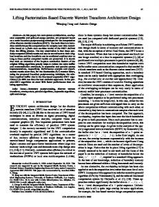
A Volterra series-assisted undecimated lifting wavelet packet transform is proposed for machinery incipient defect diagnosis to eliminate the frequency aliasing and end distortion issues in traditional lifting wavelet transform, and its flowchart is shown in Figure 1. First, both ends of the original signal are extended and predicted with Volterra series model, in which the parameter of extension number is optimized. Next, the extended signal is decomposed by undecimated lifting wavelet packet transform and the subband with the highest energy ratio is selected as the band of interest. The selected subband signal is then trimmed back to its original length for envelope analysis. Finally, the machinery status is assessed according to the analysis results. The details of undecimated lifting wavelet packet transform with boundary treatment are discussed as below. 3.1. Formulation of Undecimated LWPT with Boundary Treatment. The undecimated algorithm can eliminate frequency aliasing because the length of coefficients at each level is equal to that of the raw signal. The P and U can be schemed out as initial prediction operator and initial update operator, respectively, and the undecimated algorithm is deduced as follows. Assuming P = {𝑝𝑖 }, where 𝑖 = 1, 2, . . . , 𝑁, the expression of the undecimated prediction operator of the 𝑙th level is given by [34] {𝑝𝑖 , P[𝑙] 𝑗 ={ 0, {
𝑗 = 2𝑙 ⋅ 𝑖, 𝑗 ≠ 2𝑙 ⋅ 𝑖,
𝑗 = 1, . . . , 2𝑙 𝑁.
(11)
4
Shock and Vibration
15
10
10
5
5
0
0
−5
−5
−10
−10
−15
0
0.01
−15
0.02 0.03 0.04 Data acquisition
0 −2 −4 −6 −8
Status assessment
0
0.01 0.02 0.03 0.04 0.05 0.06 Volterra series model
Parameter optimization
1 0 −1 0 10 0 −10 0 1 0 −1 0 10 0 −10 0
0
0.01 0.02 0.03 0.04 0.05 0.06 0.07 Time t (s) Envelope analysis
4 2
0.05
0.1
0.15
0.2
0.25
0.05
0.1
0.15
0.2
0.25
0.05
0.1
0.15
0.2
0.25
0.05 0.1 0.15 0.2 Undecimated LWPT
0.25
X43
2
Undecimated update operator: U
0 −2
X42
4
Extension number: nadd
Undecimated prediction operator: P
6
6
Amplitude a (mm·s−2 )
Amplitude a (mm·s−2 )
8
Prediction coefficient: W(n)
−4 −6 0
0.05
0.1 0.15 0.2 Time t (s) Data trimming
X41
Machinery
Extension signal
X44
15
0.25
Figure 1: Flowchart of the proposed approach for machinery incipient defect diagnosis.
According to the principle of equidistance subdivision, the predictor coefficient 𝑝𝑖 is calculated by Lagrange interpolation formula as [29] 𝑁
𝑝𝑖 = ∏ 𝑘=1 𝑘=𝑖̸
(𝑁 + 1) /2 − 𝑘 , 𝑖−𝑘
𝑖 = 1, 2, . . . , 𝑁,
(12)
where 𝑖 is an index number and 𝑁 is the predictor length. Similarly, assuming U = {𝑢𝑖 }, where 𝑖 = 1, 2, . . . , 𝑁 , the expression of the undecimated update operator of the 𝑙th level is obtained by [34] {𝑢𝑖 , U[𝑙] 𝑗 ={ 0, {
𝑗 = 2𝑙 ⋅ 𝑖,
𝑗 = 1, . . . , 2𝑙 𝑁 ,
𝑗 ≠ 2𝑙 ⋅ 𝑖,
− [𝑝1[𝑙] 𝑥(𝑙−1)(𝑘/2) (𝑛 − 2𝑙−1 (𝑁 + 1) + 1)
+
𝑢2[𝑙] 𝑥𝑙(𝑘−1)
𝑙−1
(𝑛 − 2
(𝑁 + 1) + 2) + ⋅ ⋅ ⋅
𝑙−1 (𝑁 − 1))] , + 𝑢2[𝑙]𝑙 𝑁 ̃ 𝑥𝑙(𝑘−1) (𝑛 + 2
It can be deduced that three numbers must be extended to the left end of 𝑥 when calculating 𝑑1,1 and the same number to the right when calculating the last data 𝑑1,𝑛 . Similarly, for the second level, 6 more numbers should be extended to each end, and so on. More generally, assuming 𝑁𝑓 is the decomposed level of undecimated lifting wavelet packet transform, the extension number of the original signal at each end can be calculated as 𝑁𝑓
𝑛add = ∑ [2𝑙−1 (𝑁 + 1) − 1]
+ 𝑝2[𝑙] 𝑥(𝑙−1)(𝑘/2) (𝑛 − 2𝑙−1 (𝑁 + 1) + 2) + ⋅ ⋅ ⋅
+ [𝑢1[𝑙] 𝑥𝑙(𝑘−1) (𝑛 − 2𝑙−1 (𝑁 + 1) + 1)
(15)
(13)
𝑥𝑙(𝑘−1) (𝑛) = 𝑥(𝑙−1)(𝑘/2) (𝑛)
𝑥𝑙𝑘 (𝑛) = 𝑥(𝑙−1)(𝑘/2) (𝑛)
𝑑1,𝑖 = 𝑥𝑖 − (𝑥𝑖−3 × 𝑝1 + 𝑥𝑖−2 × 0 + 𝑥𝑖−1 × 𝑝2 + 𝑥𝑖 × 0 + 𝑥𝑖+1 × 𝑝3 + 𝑥𝑖+3 × 𝑝4 ) .
where 𝑢𝑖 is the update coefficient and is usually set as the half of the predictor coefficient 𝑝𝑖 . Assuming 𝑥𝑙𝑘 is the 𝑘th frequency band of the 𝑙th level signal decomposed from the original signal 𝑥[𝑛], 𝑥𝑙(𝑘−1) and 𝑥𝑙𝑘 can be obtained by dividing 𝑥(𝑙−1)(𝑘/2) ,
+ 𝑝2[𝑙]𝑙 𝑁𝑥(𝑙−1)(𝑘/2) (𝑛 + 2𝑙−1 (𝑁 − 1))] ,
where 𝑘 = 2, 4, 6, . . . , 2𝑙 ; 𝑝𝑖[𝑙] is the undecimated prediction operator of 𝑥𝑙(𝑘−1) ; and 𝑢𝑖[𝑙] is the undecimated update operator of 𝑥𝑙𝑘 . Assuming the undecimated prediction operator P = {𝑝𝑖 } and the undecimated update operator U = {𝑢𝑖 }, where 𝑖 = 1, 2, . . . , 4, 𝑥𝑖 is the 𝑖th data of X. The 𝑖th data of the first level detailed signal decomposed by undecimated lifting wavelet packet transform is obtained as follows:
𝑙=1
𝑁𝑓
(14)
(16)
+ ∑ [2𝑙−1 (𝑁 + 1) − 1] . 𝑙=1
According to (16), the length of extended signal in Volterra series model is determined, and the signal is extended based on the procedure of Volterra series model in Section 2. The performance of formulated method is discussed below.
Shock and Vibration
5
0.3
End distortion
End distortion
0.1
0
−0.1
Amplitude a (mm·s−2 )
Amplitude a (mm·s−2 )
2
Characteristic signal
0.2
Characteristic signal 1
End distortion
End distortion 0
−1
−2
−0.2 0
0.02
0.04
0.06 Time t (s)
0.08
0.1
0.12
0
0.02
0.04
(a)
0.06 Time t (s)
0.08
0.1
0.12
(b)
0.3 8
4
Characteristic signal
0.2
Characteristic signal End distortion
2 0 −2 −4
Amplitude a (mm·s−2 )
Amplitude a (mm·s−2 )
6
0.1 0 −0.1 −0.2
−6 −8 0
0.02
0.04
0.06 Time t (s)
0.08
0.1
0.12
(c)
0
0.02
0.04
0.06 Time t (s)
0.08
0.1
0.12
(d)
Figure 2: One subband in the fourth layer decomposed using wavelet packet and preprocessed by different methods: (a) no extension, (b) zero-padding extension, (c) periodic extension, and (d) second-order Volterra series prediction.
3.2. Performance Comparison of Boundary Treatment Methods. To evaluate the performance of various boundary treatment methods, a synthesized signal is constructed as follows: 𝑥 (𝑡) = 0.3 exp (−2𝜋 × 100𝑡) sin (2𝜋 × 400𝑡) + 1.5 sin (2𝜋 × 50𝑡 +
𝜋 ) 4
+ 3 sin (2𝜋 × 100𝑡 +
𝜋 ). 6
located in the end, it will be submerged by the end distortions. In Figures 2(b)-2(c), the characteristic signal in the middle is insignificant because the end distortion is strong. The Volterra series based preprocessing method shows the optimal performance since the end distortions have been restrained effectively as shown in Figure 2(d).
(17)
The sampling frequency is set as 16,000 Hz. The synthesized signal is decomposed into four layers using the undecimated lifting wavelet transform. Figure 2 shows one subband of the fourth layer, corresponding to the pulse train signal, under different preprocessing scenarios, (a) no extension, (b) zeropadding extension, (c) periodic extension, and (d) secondorder Volterra series prediction, respectively. There are obvious end distortions shown by the arrows in Figures 2(a)–2(c). Therefore, if the characteristic signal is just
4. Experimental Study A reciprocating compressor (model number 4HOS-6) in a petrochemical plant in China is used as the experimental testbed to evaluate the performance of the developed method, as shown in Figure 3. It is a 4-cylinder natural gas reciprocating compressor driven by an 8-cylinder gas engine with rated power of 1,600 kW. The rotating speed of crankshaft is 860 rpm which drives the plungers to strike 860 times per minute, back and forth. The motion of the plungers changes the volume of the cylinders. When the plunger moves down, the increased volume of cylinder opens intake valve and
6
Shock and Vibration 4th cylinder
1
4
2
3
3rd cylinder
Natural gas engine
Crankshaft box
1st cylinder
Accelerometer (in the bottom)
2nd cylinder
(a)
(b)
5 0 −5 −10 0
Periodic impact 0.05 0.1
0.15
Periodic impact 0.2 0.25
Amplitude a (mm·s−2 )
Amplitude a (mm·s−2 )
Figure 3: Illustration of experimental setup, (a) data acquisition system, A control panel, B data acquisition box, C accelerometer on the exhaust valve lid, D exhaust valve, and (b) diagram of reciprocating compressor.
15 10 5 0 −5 −10 −15
0
0.05
0.1
Time t (s)
Figure 4: The time series vibrational signal of normal valve.
0.15 Time t (s)
0.2
0.25
Figure 5: The time series vibrational signal of abnormal valve. Level 1
closes the exhaust valve. When the plunger moves up, the compression of cylinder opens the exhaust valve and closes the intake valve. Valve is composed of lifting limiter, spring, disc, and seat, of which spring is the most susceptible to failure. To diagnose the valve failure in the 2nd cylinder, an accelerometer is placed on the exhaust valve lid. A customer designed data acquisition system (model number MDES-5) as shown in Figure 3(a) is used to acquire the measurements. It consists of a laptop and a data acquisition box configured in a master-slave system. The sampling rate is set as 16 kHz in this study. Figures 4 and 5 show the time series vibrational signals near the exhaust valve of 2nd cylinder under normal condition and abnormal condition, respectively. For comparison, the amplitude of the vibration signal under abnormal condition is greater than the one of the normal signal. Taking the RMS (root mean square) as the criterion, the RMS of the abnormal signal is calculated as 4.725 m⋅s−2 which is greater than that of the normal signal (2.227 m⋅s−2 ). However, the periodic impact feature caused by the collision of the valve disc and seat is difficult to observe due to strong background noise. For further analysis, the proposed method based on Volterra series and undecimated lifting wavelet packet transform is used to process the signals. The two ends of the original signal are extended and predicted by the Volterra series model. Then, the predicted signal is decomposed into four
100 50 0
97.30 2.70
1
2 Level 2
100 50 0
69.28 7.36
0.07
23.29
1
2
3
4
Level 3
100 50 0
0.63
4.26
0.12
0.01
12.59
10.79
1
2
3
4
5
6
40.39
31.21
7
8
Level 4
100 50 0
22.62 14.48 28.83 5.75 0.84 0.06 2.40 1.44 0.04 0.05 0.01 0.00 7.64 4.07 8.99 2.79
0
2
4
6
8
10
12
14
16
Figure 6: Energy distribution of four-level subbands.
layers by undecimated lifting wavelet packet transform, where 𝑁 = 𝑁 = 4. From (11)–(13), the prediction operator P and the update operator U can be obtained as P = [−0.0625, 0.5625, 0.5625, −0.0625] and U = [−0.0313, 0.2813, 0.2813, −0.0313]. Finally, the 16 subbands of the fourth level are obtained and the energy distribution of the subbands at different levels is shown in Figure 6. After undecimated lifting wavelet packet decomposition, the majority of the energy rests on the high frequency parts which
Amplitude a (mm·s−2 )
Shock and Vibration 8 6 4 2 0 −2 −4 −6 −8 0
Amplitude a (mm·s−2 )
7
0.05
0.1 0.15 Time t (s) (a)
0.2
0.25
8 6 4 2 0 −2 −4 −6 −8 0.02
0.03
0.04
0.05 0.06 Time t (s) (b)
0.07
0.08
Amplitude a (mm·s−2 )
Figure 7: The wavelet coefficient at selected subband and its envelope under normal condition.
6 4 2 0 −2 −4 −6 0
0.05
0.1
0.15
0.2
0.25
Amplitude a (mm·s−2 )
Time t (s) (a) 8 6 4 2 0 −2 −4 −6 −8 0.02
0.03
0.04
0.05
0.06
0.07
0.08
Time t (s) (b)
Figure 8: The wavelet coefficient at selected subband and its envelope under abnormal condition.
correspond to the detailed wavelet coefficients. The subband with the highest energy ratio is selected as the band of interest. The wavelet coefficients and their envelopes from the selected subbands are shown in Figures 7 and 8, corresponding to the normal condition and abnormal condition, respectively. From both figures, the periodic impact features are visible and easily identified. The signal in one period, as shown by the red block in Figures 7(a) and 8(a), is extracted for detailed analysis. According to the working principle of exhaust valve, the front
half curve, from 0.012 to 0.047 sec, represents the valve-close phase while the latter one, from 0.047 to 0.082 sec, shows the exhaust phase. The exhaust valve closes at point A, and the valve opens again at point B. Under normal condition, there is no chattering when normal valve closes because the stiffness of spring is rigid enough to close tightly. By contrast, valve chatters significantly which is caused by the repeated collision of valve and seat during the time period 𝑇 (indicating the aging and stretch decline of spring in the valve). The valve with aged spring cannot close tightly resulting in gas leak and efficiency degradation. When this compressor is stopped and checked, the spring failure is validated by visual inspection, and the exhaust valve is maintained. Therefore, the presented incipient fault diagnosis method avoids accidents and prevents huge production loss. In addition, the energy of the selected band signal is used to evaluate the performance of the presented method. Figure 9(a) shows the energies of the selected band signals under four different scenarios: (I) undecimated LWPT (ULWPT) under normal machinery condition, (II) undecimated LWPT (ULWPT) under abnormal machinery condition, (III) Volterra series assisted undecimated LWPT (V-ULWPT) under normal machinery condition, and (IV) Volterra series assisted undecimated LWPT (V-ULWPT) under abnormal machinery condition. From the analysis results, it is found that the normal and abnormal machinery conditions can be differentiated according to energy of selected subband using undecimated lifting wavelet packet transform. Since Volterra series assisted ULWPT suppresses the end distortion, the energy of selected subband using VULWPT is less than that using ULWPT. However, the energy ratio of abnormal to normal conditions using V-ULWPT is larger than that using ULWPT as shown in Figure 9(b), thus validating the effectiveness of presented Volterra series assisted lifting wavelet packet transform method. The computational efficiency of the developed technique has also been evaluated on a desktop (Lenovo Yangtian T4900d model, Lenovo Inc., Beijing, China) with a 3.3 GHz CPU and 4 GB memory. It takes approximately 1.19 seconds to process a data string containing 4,096 data points, which is equivalent to processing 0.256 seconds data length under a 16 kHz sampling rate. Thus the presented method is applicable for online machinery diagnosis in practical applications.
5. Conclusions An enhanced weak feature extraction approach that combines Volterra series model and undecimated lifting wavelet packet transform has been presented for incipient fault detection. The analysis results show that Volterra series assisted undecimated lifting wavelet packet transform eliminates the frequency aliasing and end distortion issues in conventional lifting wavelet packet transform method; thus it is significant to machinery incipient defect diagnosis, especially for weak impact feature extraction. From the engineering application perspective, the weak impact signals caused by the fault of a valve in reciprocating compressor are analyzed using the presented method, and the early spring failure is detected from the extracted weak features using the presented method.
8
Shock and Vibration 4
6.00E + 03 5.50E + 03
3.5
5.00E + 03 4.50E + 03
3
4.28E + 03 Energy ratio
Energy (J)
4.00E + 03 3.50E + 03 3.00E + 03 2.50E + 03 2.19E + 03 2.00E + 03 1.36E + 03
1.50E + 03
2.5 2.16 2 1.5 1
1.00E + 03
0.5
5.00E + 02 0.00E + 00
3.14
4.75E + 03
0 I
II
III
I: normal ULWPT III: normal V-ULWPT
IV
II: abnormal ULWPT IV: abnormal V-ULWPT
(a)
I
II
I: ULWPT abnormal/normal II: V-ULWPT abnormal/normal (b)
Figure 9: Energy comparison among different conditions: (a) energy comparison chart, (b) energy ratio chart.
Conflict of Interests The authors declare that there is no conflict of interests regarding the publication of this paper.
Acknowledgments This research acknowledges the financial support provided by National Science foundation of China (no. 51504274), Science Foundation of China University of Petroleum, Beijing (nos. 2462014YJRC039 and 2462015YQ0403), and Beijing Municipal Education Commission Cooperative Construction Project. Valuable comments from anonymous reviewers are greatly appreciated.
References [1] V. Venkatasubramanian, R. Rengaswamy, K. Yin, and S. N. Kavuri, “A review of process fault detection and diagnosis: part I: quantitative model-based methods,” Computers and Chemical Engineering, vol. 27, no. 3, pp. 293–311, 2003. [2] M. Liang and I. S. Bozchalooi, “An energy operator approach to joint application of amplitude and frequency-demodulations for bearing fault detection,” Mechanical Systems and Signal Processing, vol. 24, no. 5, pp. 1473–1494, 2010. [3] Z. Zhong, Z. Jiang, Y. Long, and X. Zhan, “Analysis on the noise for the different gearboxes of the heavy truck,” Shock and Vibration, vol. 2015, Article ID 476460, 5 pages, 2015. [4] W. J. Wang, “Wavelet transform in vibration analysis for mechanical fault diagnosis,” Shock and Vibration, vol. 3, no. 1, pp. 17–26, 1996. [5] Y. Lei, J. Lin, Z. He, and M. J. Zuo, “A review on empirical mode decomposition in fault diagnosis of rotating machinery,” Mechanical Systems and Signal Processing, vol. 35, no. 1-2, pp. 108–126, 2013.
[6] N. Baydar and A. Ball, “A comparative study of acoustic and vibration signals in detection of gear failures using Wigner-Ville distribution,” Mechanical Systems and Signal Processing, vol. 15, no. 6, pp. 1091–1107, 2001. [7] W.-X. Yang and P. W. Tse, “Development of an advanced noise reduction method for vibration analysis based on singular value decomposition,” NDT & E International, vol. 36, no. 6, pp. 419– 432, 2003. [8] H. Hassanpour, A. Zehtabian, and S. J. Sadati, “Time domain signal enhancement based on an optimized singular vector denoising algorithm,” Digital Signal Processing, vol. 22, no. 5, pp. 786–794, 2012. [9] J. Wang, R. X. Gao, and R. Yan, “Integration of EEMD and ICA for wind turbine gearbox diagnosis,” Wind Energy, vol. 17, no. 5, pp. 757–773, 2014. [10] A. Sadhu and B. Hazra, “A novel damage detection algorithm using time-series analysis-based blind source separation,” Shock and Vibration, vol. 20, no. 3, pp. 423–438, 2013. [11] Z. K. Peng and F. L. Chu, “Application of the wavelet transform in machine condition monitoring and fault diagnostics: a review with bibliography,” Mechanical Systems and Signal Processing, vol. 18, no. 2, pp. 199–221, 2004. [12] R. Yan, R. X. Gao, and X. Chen, “Wavelets for fault diagnosis of rotary machines: a review with applications,” Signal Processing, vol. 96, pp. 1–15, 2014. [13] N. Saravanan and K. I. Ramachandran, “Incipient gear box fault diagnosis using discrete wavelet transform (DWT) for feature extraction and classification using artificial neural network (ANN),” Expert Systems with Applications, vol. 37, no. 6, pp. 4168–4181, 2010. [14] H. Qiu, J. Lee, J. Lin, and G. Yu, “Wavelet filter-based weak signature detection method and its application on rolling element bearing prognostics,” Journal of Sound and Vibration, vol. 289, no. 4-5, pp. 1066–1090, 2006. [15] J. Wang, R. X. Gao, and R. Yan, “Multi-scale enveloping order spectrogram for rotating machine health diagnosis,” Mechanical Systems and Signal Processing, vol. 46, no. 1, pp. 28–44, 2014.
Shock and Vibration [16] Y.-L. Chen, P.-L. Zhang, B. Li, and D.-H. Wu, “Denoising of mechanical vibration signals using quantum-inspired adaptive wavelet shrinkage,” Shock and Vibration, vol. 2014, Article ID 848097, 7 pages, 2014. [17] Y. Pan, J. Chen, and X. Li, “Bearing performance degradation assessment based on lifting wavelet packet decomposition and fuzzy c-means,” Mechanical Systems and Signal Processing, vol. 24, no. 2, pp. 559–566, 2010. [18] R. Zhou, W. Bao, N. Li, X. Huang, and D. Yu, “Mechanical equipment fault diagnosis based on redundant second generation wavelet packet transform,” Digital Signal Processing: A Review Journal, vol. 20, no. 1, pp. 276–288, 2010. [19] J. Yuan, Z. He, and Y. Zi, “Gear fault detection using customized multiwavelet lifting schemes,” Mechanical Systems and Signal Processing, vol. 24, no. 5, pp. 1509–1528, 2010. [20] Y. He, X. Chen, J. Xiang, and Z. He, “Adaptive multiresolution finite element method based on second generation wavelets,” Finite Elements in Analysis and Design, vol. 43, no. 6-7, pp. 566– 579, 2007. [21] W. Bao, R. Zhou, J. Yang, D. Yu, and N. Li, “Anti-aliasing lifting scheme for mechanical vibration fault feature extraction,” Mechanical Systems and Signal Processing, vol. 23, no. 5, pp. 1458–1473, 2009. [22] R. L. Claypoole, G. M. Davis, W. Sweldens, and R. G. Baraniuk, “Nonlinear wavelet transforms for image coding via lifting,” IEEE Transactions on Image Processing, vol. 12, no. 12, pp. 1449– 1459, 2003. [23] R. L. Claypoole, R. G. Baraniuk, and R. D. Nowak, “Adaptive wavelet transforms via lifting,” Report ECE TR-9304, 1999, https://scholarship.rice.edu/handle/1911/19808. [24] B. Appleton and H. Talbot, “Recursive filtering of images with symmetric extension,” Signal Processing, vol. 85, no. 8, pp. 1546– 1556, 2005. [25] B. Wohlberg and C. M. Brislawn, “Symmetric extension for lifted filter banks and obstructions to reversible implementation,” Signal Processing, vol. 88, no. 1, pp. 131–145, 2008. [26] L. Duan, L. Zhang, and J. Chen, “Boundary treatment of lifting wavelet transform based on Volterra series model and its application,” Chinese Journal of Scientific Instrument, vol. 33, no. 1, pp. 7–12, 2012. [27] D. Aiordachioaie, E. Ceanga, R. de Keyser, and Y. Naka, “Detection and classification of non-linearities based on Volterra kernels processing,” Engineering Applications of Artificial Intelligence, vol. 14, no. 4, pp. 497–503, 2001. [28] W. Sweldens, “The lifting scheme: a custom-design construction of biorthogonal wavelets,” Applied and Computational Harmonic Analysis, vol. 3, no. 2, pp. 186–200, 1996. [29] W. Sweldens, “The Lifting Scheme: a construction of second generation wavelets,” SIAM Journal on Mathematical Analysis, vol. 29, no. 2, pp. 511–546, 1998. [30] A. Ben and T. Hugues, “Recursive filtering of images with symmetric extension,” Signal Processing, vol. 85, no. 8, pp. 1546–1556, 2005. [31] D. Aiordachioaie, E. Ceanga, R. De Keyser, and Y. Naka, “Detection and classification of non-linearities based on Volterra kernels processing,” Engineering Applications of Artificial Intelligence, vol. 14, no. 4, pp. 497–503, 2001. [32] M. B. Kennel, R. Brown, and H. D. I. Abarbanel, “Determining embedding dimension for phase-space reconstruction using a geometrical construction,” Physical Review A, vol. 45, no. 6, pp. 3403–3411, 1992.
9 [33] J. Zhang and X. Xiao, “Predicting low-dimensional chaotic time series using Volterra adaptive filters,” Acta Physica Sinica, vol. 49, no. 3, pp. 403–408, 1999. [34] J. Hongkai, H. Zhengjia, D. Chendong, and C. Peng, “Gearbox fault diagnosis using adaptive redundant Lifting Scheme,” Mechanical Systems and Signal Processing, vol. 20, no. 8, pp. 1992–2006, 2006.
International Journal of
Rotating Machinery
Engineering Journal of
Hindawi Publishing Corporation http://www.hindawi.com
Volume 2014
The Scientific World Journal Hindawi Publishing Corporation http://www.hindawi.com
Volume 2014
International Journal of
Distributed Sensor Networks
Journal of
Sensors Hindawi Publishing Corporation http://www.hindawi.com
Volume 2014
Hindawi Publishing Corporation http://www.hindawi.com
Volume 2014
Hindawi Publishing Corporation http://www.hindawi.com
Volume 2014
Journal of
Control Science and Engineering
Advances in
Civil Engineering Hindawi Publishing Corporation http://www.hindawi.com
Hindawi Publishing Corporation http://www.hindawi.com
Volume 2014
Volume 2014
Submit your manuscripts at http://www.hindawi.com Journal of
Journal of
Electrical and Computer Engineering
Robotics Hindawi Publishing Corporation http://www.hindawi.com
Hindawi Publishing Corporation http://www.hindawi.com
Volume 2014
Volume 2014
VLSI Design Advances in OptoElectronics
International Journal of
Navigation and Observation Hindawi Publishing Corporation http://www.hindawi.com
Volume 2014
Hindawi Publishing Corporation http://www.hindawi.com
Hindawi Publishing Corporation http://www.hindawi.com
Chemical Engineering Hindawi Publishing Corporation http://www.hindawi.com
Volume 2014
Volume 2014
Active and Passive Electronic Components
Antennas and Propagation Hindawi Publishing Corporation http://www.hindawi.com
Aerospace Engineering
Hindawi Publishing Corporation http://www.hindawi.com
Volume 2014
Hindawi Publishing Corporation http://www.hindawi.com
Volume 2014
Volume 2014
International Journal of
International Journal of
International Journal of
Modelling & Simulation in Engineering
Volume 2014
Hindawi Publishing Corporation http://www.hindawi.com
Volume 2014
Shock and Vibration Hindawi Publishing Corporation http://www.hindawi.com
Volume 2014
Advances in
Acoustics and Vibration Hindawi Publishing Corporation http://www.hindawi.com
Volume 2014