Wavelet Transform and Three-Dimensional Data ...

D OCTORAL T HESIS Universit`a degli studi di Napoli “Federico II”

Universit´e de Nice-Sophia Antipolis

Dipartimento di Ingegneria Elettronica e delle Telecomunicazioni

Facult´e de Science et Techniques ´ Ecole doctorale Sciences et Technologies de l’Information et de la Communication

Dottorato di Ricerca in Tecnologie dell’Informazione e della Comunicazione

AND

Discipline: automatique, traitement du signal et des images

WAVELET T RANSFORM T HREE -D IMENSIONAL D ATA C OMPRESSION defended by Marco CAGNAZZO in front of the commission composed by Luigi PAURA

Supervisors

Giovanni P OGGI Michel B ARLAUD Marc A NTONINI

Full Professor at the University of Napoli “Federico II” (Italy) Full Professor at the University of Napoli “Federico II” (Italy) Full Professor at the University of Nice-Sophia Antipolis (France) Charg´e de Recherche at the CNRS (France)

ACADEMIC YEAR

2003–2004

Acknowledgements A doctoral thesis is a three-years long work which requires the efforts of many people (beside the candidate himself/herself) in order to be completed. My case was not an exception, as many people helped me in many ways during these years. I owe acknowledgements to all of them. I firstly would like to thanks professor Luigi Paura, whose hard work made it possible to start an international doctoral program at the “Federico II” University of Napoli (Italy). This effort is mirrored by that done by professor Michel Barlaud at the “Universit´e de Nice-Sophia Antipolis” (France). I owe a deep thank to my supervisors, who directed my research work with extreme competence, and gave me many useful hints, indications and suggestions, without which I would not have been able to accomplish this thesis work. So thank you, professors Giovanni Poggi, (Universit`a “Federico II”), Michel Barlaud and Marc Antonini (I3S Laboratory, France). In these three years I met many people, whose collaboration gave a incredible speed-up to my research work. So I thank Dr. Annalisa Verdoliva and Giuseppe Scarpa (at the “Federico II” University), Andrea Zinicola (at CNIT Laboratory of Napoli), Dr. Christophe Parisot, Valery Val´entin, Federico Matta, Thomas Andr´e, Muriel Gastaud, Dr. Fr´ed´eric Precioso, Dr. Eric Debreuve, Vincent Garcia (at the I3S Laboratory). I would like to spend some more word for some of my colleagues. Thank you Annalisa for your collaboration, for so many hints and suggestions, for all the interesting discussions we have had, and above all for your friendship. Thank you Donatella for all the times we have talked about books, research, movies, university, life. And thank you Peppe, you are my reference in football, segmentation, cooking, “prince behavior” (together with Franco, who deserves many thanks as well): thank you for many priceless hints and “real life”-theorems (as the Peppe’s first theo-

ii

A CKNOWLEDGEMENTS

rem and its corollary, which I proved true in several occasions). I owe a special thank to Thomas, an excellent colleague and a very good friend: it has been a real pleasure to work with you. And, last but not least, I want to thank my French teacher, the Linux-addicted and LATEX-fundamentalist Lionel, who let me never feel abroad, and helped me so many times that I can hardly remember. A very special thank goes to Coralie, who gave me an extraordinary support in recent times. The last words go to my family, who always and more than ever has supported me in this path to the last part of my student life. Thanks to my sister Paola and to Ivano, and of course to my parents, to whom I owe everything. Thank you all!

Napoli, January 2005

Contents Acknowledgements

i

Contents

iii

Preface

vii

Introduction

ix

1

Video Coding 1.1 Hybrid Video Coding . . . . . . . . . . . . . . . . . . . . . . . 1.2 Wavelet Transform Based Video Coding . . . . . . . . . . . . 1.3 Video Coding for Heterogeneous Networks . . . . . . . . . .

2

Proposed Encoder Architecture 2.1 Why a new video encoder? . . . . . . 2.2 General Encoder Structure . . . . . . . 2.3 Temporal Analysis . . . . . . . . . . . 2.3.1 Temporal Filtering . . . . . . . 2.3.2 Motion Estimation . . . . . . . 2.3.3 Motion Vector Encoding . . . . 2.4 Spatial Analysis . . . . . . . . . . . . . 2.4.1 Spatial Filtering and Encoding 2.4.2 Resource Allocation . . . . . . 2.5 Open Issues . . . . . . . . . . . . . . .

3

1 2 4 8

. . . . . . . . . .

11 11 14 14 15 16 16 17 17 17 18

Temporal Filtering 3.1 Temporal Filtering for Video Coding . . . . . . . . . . . . . . 3.2 Lifting Scheme and Temporal Transform . . . . . . . . . . . .

21 21 24

. . . . . . . . . .

. . . . . . . . . .

. . . . . . . . . .

. . . . . . . . . .

. . . . . . . . . .

. . . . . . . . . .

. . . . . . . . . .

. . . . . . . . . .

. . . . . . . . . .

. . . . . . . . . .

. . . . . . . . . .

. . . . . . . . . .

iv

C ONTENTS 3.3 3.4 3.5

4

5

6

Motion Compensated (2,2) Lifting Scheme . . . . . . . . . . . 26 ( N, 0) Filters . . . . . . . . . . . . . . . . . . . . . . . . . . . . 29 Implementation Issues . . . . . . . . . . . . . . . . . . . . . . 31

Motion Estimation Issues 4.1 A Brief Overview of Motion Estimation . . . . . . 4.2 Block Based Motion Estimation . . . . . . . . . . . 4.3 Constrained Motion Estimation . . . . . . . . . . . 4.4 Regularized Motion Estimation . . . . . . . . . . . 4.5 Optimal ME for WT-based Video Coding . . . . . 4.5.1 Notation . . . . . . . . . . . . . . . . . . . . 4.5.2 Optimal Criterion . . . . . . . . . . . . . . . 4.5.3 Developing the Criterion for a Special Case Motion Vector Encoding 5.1 Motion Vector Distribution . . . . . . . . . . . . 5.2 Encoding Techniques: Space Compression . . . 5.2.1 Experimental Results . . . . . . . . . . . 5.3 Encoding Techniques: Time Compression . . . 5.3.1 Experimental Results . . . . . . . . . . . 5.4 Validation of MVF Coding Techniques . . . . . 5.4.1 Experimental Results . . . . . . . . . . . 5.5 Vector Representation via Energy and Position 5.6 Scalable Motion Vector Encoding by WT . . . . 5.6.1 Technique Description . . . . . . . . . . 5.6.2 Proposed Technique Main Features . . Space Analysis and Resource Allocation 6.1 Spatial Filtering and Encoding . . . 6.2 The Resource Allocation Problem . . 6.3 Solutions for the Allocation Problem 6.4 Rate Allocation Problem . . . . . . . 6.5 Distortion Allocation Problem . . . . 6.6 Model-Based RD Curve Estimation . 6.7 Scalability Issues . . . . . . . . . . . 6.7.1 Bit-rate Scalability . . . . . . 6.7.2 Temporal Scalability . . . . . 6.7.3 Spatial Scalability . . . . . . .

. . . . . . . . . .

. . . . . . . . . .

. . . . . . . . . .

. . . . . . . . . .

. . . . . . . . . .

. . . . . . . . . .

. . . . . . . . . . . . . . . . . . . . .

. . . . . . . . . . . . . . . . . . . . .

. . . . . . . . . . . . . . . . . . . . . . . . . . . . .

. . . . . . . . . . . . . . . . . . . . . . . . . . . . .

. . . . . . . . . . . . . . . . . . . . . . . . . . . . .

. . . . . . . . . . . . . . . . . . . . . . . . . . . . .

. . . . . . . . . . . . . . . . . . . . . . . . . . . . .

. . . . . . . .

37 37 43 46 49 52 53 54 57

. . . . . . . . . . .

59 60 61 69 72 73 75 75 79 81 81 82

. . . . . . . . . .

87 87 89 91 93 96 97 99 101 101 104

C ONTENTS 6.8 7

v

Experimental Results . . . . . . . . . . . . . . . . . . . . . . . 105

Optimal Resource Allocation 7.1 Problem definition . . . . . . . . . . . . . . 7.2 General Formulation . . . . . . . . . . . . . 7.3 Separated Allocation . . . . . . . . . . . . . 7.3.1 The σ2 ( RMV ) Function . . . . . . . . 7.4 Global Allocation . . . . . . . . . . . . . . . 7.4.1 Models and Estimation for σi2 ( RMV ) 7.5 Non-Asymptotic Analysis . . . . . . . . . . 7.6 Conclusion . . . . . . . . . . . . . . . . . . .

. . . . . . . .

109 109 111 112 115 118 121 122 123

8

Low Complexity Video Compression 8.1 Complexity Issues in Video Coding . . . . . . . . . . . . . . . 8.2 The Chaddha-Gupta Coder . . . . . . . . . . . . . . . . . . . 8.3 Proposed Improvements . . . . . . . . . . . . . . . . . . . . . 8.3.1 Ordered Codebooks . . . . . . . . . . . . . . . . . . . 8.3.2 Index-based Conditional Replenishment . . . . . . . 8.3.3 Index-predictive Vector Quantization . . . . . . . . . 8.3.4 Table Lookup Filtering and Interpolation . . . . . . . 8.3.5 Computational Complexity of the Proposed Scheme . 8.4 Experimental Results . . . . . . . . . . . . . . . . . . . . . . .

125 125 127 129 129 131 131 132 133 134

9

SAR Images Compression 9.1 SAR Images: An Object-Oriented Model 9.2 Image Model and Coding Schemes . . . 9.3 Numerical Results . . . . . . . . . . . . . 9.4 Conclusions . . . . . . . . . . . . . . . .

. . . .

137 137 140 141 145

. . . . . . . .

147 147 152 153 154 157 158 161 162

. . . .

10 Multispectral & Multitemporal Images 10.1 Multispectral Images Compression . . . . 10.1.1 Segmentation . . . . . . . . . . . . 10.1.2 Map coding . . . . . . . . . . . . . 10.1.3 Shape-adaptive wavelet transform 10.1.4 Shape-adaptive SPIHT . . . . . . . 10.1.5 Rate allocation . . . . . . . . . . . 10.1.6 Implemented Techniques . . . . . 10.1.7 Experimental results . . . . . . . .

. . . . . . . . . . . .

. . . . . . . .

. . . . . . . . . . . .

. . . . . . . .

. . . . . . . . . . . .

. . . . . . . .

. . . . . . . . . . . .

. . . . . . . .

. . . . . . . . . . . .

. . . . . . . .

. . . . . . . . . . . .

. . . . . . . .

. . . . . . . . . . . .

. . . . . . . .

. . . . . . . . . . . .

. . . . . . . .

. . . . . . . . . . . .

. . . . . . . .

. . . . . . . . . . . .

vi

C ONTENTS 10.2 Multitemporal Image Compression . . . . . . . 10.2.1 Classification . . . . . . . . . . . . . . . 10.2.2 Change detection map and map coding 10.2.3 Texture coding . . . . . . . . . . . . . . 10.2.4 Numerical results . . . . . . . . . . . . . 10.3 Conclusion . . . . . . . . . . . . . . . . . . . . .

. . . . . .

. . . . . .

. . . . . .

. . . . . .

. . . . . .

. . . . . .

. . . . . .

. . . . . .

A Coding Gain for Biorthogonal WT

168 170 171 172 173 174 177

B Allocation Algorithm Results 183 B.1 Colour Management . . . . . . . . . . . . . . . . . . . . . . . 183 C Video Bitstream Structure and Scalability issues C.1 Sequence Level Structure . . . . . . . . . . . . . . . . . . . . . C.2 Subband Level Structure . . . . . . . . . . . . . . . . . . . . . C.3 Image Level Structure . . . . . . . . . . . . . . . . . . . . . .

187 188 189 191

D List of Abbreviations

195

Bibliography

197

Index

208

Summary

211

R´esum´e

213

Preface This Ph.D. thesis work was carried on in the form of a cotutelle between the “Federico II” University of Napoli (Italy) and the “Universit´e de NiceSophia Antipolis” of Nice (France). Namely, I worked in the “Dipartimento d’Ingegneria Elettronica e delle Telecomunicazioni” of the Napoli University, under the guidance of professor Giovanni Poggi, from January 2002 till December 2002, and from April 2004 till December 2004. I was also at the “I3S” Laboratory of Sophia Antipolis, from January 2003 till March 2004 (plus a week in November 2002, one in May 2004, and a last one in October 2004), under the guidance of professors Michel Barlaud and Marc Antonini.

Introduction The leitmotiv which characterizes this Ph.D. Thesis work has been visual data compression. In fact, my work followed two main streams, wavelet based video compression and multispectral and multitemporal image compression, even though I worked briefly on low complexity video compression and SAR image compression as well. This division, between compression of video and remote sensed images, mirrors the binary structure of my Ph.D. program, which has been developed between Napoli University (Italy) and Nice-Sophia Antipolis University (France), in the framework of a cotutelle doctoral project. The topic I spent most of the time on, has been wavelet video compression, at the University of Nice, while my time at Napoli University was shared among the remaining topics, with a clear priority to the multispectral image compression problem. With the exception of low complexity video coding and SAR image compression (on which anyway I worked only for a short period), the common framework of this thesis has been the three-dimensional transform approach. In particular, my work focused on three-dimensional Wavelet Transform (WT), and its variations, such as Motion-Compensated WT or Shape-Adaptive WT. This approach can appear natural, as both video sequences and multispectral images are three-dimensional data. Nevertheless, in the video compression field, 3D-transform approaches have just begun to be competitive with hybrid schemes based on the Discrete Cosine Transform (DCT), while, as far as multispectral images are concerned, scientific literature misses a comprehensive approach to the compression problem. The 3D WT approach investigated in this thesis has drawn a huge attention by researchers in the data compression field because they hoped it could reply the excellent performances its two-dimensional version achieved in still image coding [4, 74, 81, 90, 92]. Moreover, the WT approach provides a full support for scalability, which seems to be one of

x

I NTRODUCTION

the most important topics in the field of multimedia delivery research. In a nutshell, a scalable representation of some information (images, video, . . . ) is made up of several subsets of data, each of which is an efficient representation of the original data. By taking all the subsets, one has the “maximum quality” version of the original data. By taking only some subsets, one can adjust several reproduction parameters (i.e. reduce resolution or quality) and save the rate corresponding to discarded layers. Such an approach is mandatory for efficient multimedia delivery on heterogeneous networks [56]. Another issue which is common to video and multispectral image coding, is the resource allocation problem which, in a very general way, can be described as follows. Let us suppose to have M random processes X1 , X2 . . . , X M to encode, and a given encoding technique. The resource allocation problem consists of finding a rate allocation vector, R∗ = { Ri∗ }iM =1 such that, when Xi is encoded with the given encoding technique at the bit-rate Ri∗ for each i ∈ {1, 2, . . . , M }, then a suitable cost function is minimized while certain constraints are satisfied. This allocation is then optimal for the chosen encoding technique and cost function. These random processes can be the spatiotemporal subbands resulting from three-dimensional wavelet transform of a video sequence, as well as the objects into which a multi spectral image can be divided. In both cases the problem allows very similar formulation and then very similar solution. The approach we followed is based on Rate-Distortion (RD) theory, and allows an optimal solution of the resource allocation problem, given that it is possible to know or to estimate RD characteristics of the processes. In the first part of this thesis, the video coding problem is addressed, and a new video encoder is described, which aims at full scalability without sacrificing performances, which end up being competitive with those of most recent standards. Moreover, we set the target of achieving a deep compatibility with the JPEG2000 standard. Many problems have to be solved in order to fulfil these objectives, and the solutions we propose are the core of the first part of this thesis. The last chapter of the first part deals with low complexity video coding. Here the problem is to develop a video encoder capable of a full scalability support but with an extremely reduced complexity, for real-time encoding and decoding on low resource terminals. In this framework it is not possible to perform such demanding operations as motion estimation or motion compensation, and then temporal compression is performed by

I NTRODUCTION

xi

means of conditional replenishment. My attention was then directed to a special form of Vector Quantization (VQ) [30] called hierarchical vector quantization, which allows to perform spatial compression with extremely low complexity. The main contributions in this problem lie in the introduction of several table-lookup encoding steps, Address Vector Quantization (AVQ) and predictive AVQ, and in the development of a multiplicationfree video codec. The second part of this work is about multispectral and SAR image compression. The first topic has been approached with the aim of defining a comprehensive framework with the leading idea of defining a more accurate model of multispectral images than the usual one. This model assumes that these images are made up of a small number of homogenous objects (called regions). An efficient encoder should be aware of this characteristic and exploit it for compression. Indeed, in the proposed framework, multispectral images are firstly subdivided into regions by means of a suitable segmentation algorithm. Then, we use an objected-oriented compression technique to encode them, and finally we apply a resource allocation strategy among objects. The model proposed for Multispectral images, partially matches the one for SAR images, in the sense that SAR images as well usually consists in homogeneous regions. On the other hand, these images are characterized by multiplicative noise called speckle, which makes harder processing (and in particular, compression). Filtering for noise reduction is then an almost mandatory step in order to compress these images. Anyway a too strong filter would destroy valuable information as region boundaries. For these reasons, an object based approach, preserving object boundaries and allowing an effective de-noising could bring in several advantages.

Notation Let us define some notation and conventions used throughout the thesis. As far as data compression is concerned, we can define the performance of a generic algorithm by providing the quality of reconstructed data and the cost at which it comes. Note that, in the case of lossless compression, in which reconstructed data perfectly match the original, only the coding cost is of concern. This cost is measured in bits per pixel (bpp) in the case of single-component images:

xii

I NTRODUCTION

Nb Np where Nb is the number of bit in the encoded stream and Np is the number of pixel of the original image. For multi-component images we usually use the same measure, where Np refers now to the number of pixel of a single component. In the case of multispectral and multitemporal images, all components (or bands) have the same dimensions, and sometimes this expression of rate is said to be in bit per band (bpb). When color images are concerned, we still use the same definition, but now Np refers to the largest (i.e. luminance) component dimension, since different components can have different sizes, as for images in 4 : 2 : 0 color spaces. For video, the rate is usually expressed in bit per second (bps) and its multiples as kbps, and Mbps. Rbpp =

Nb T Nb F = Nf Nb = Np F N f Np = R¯ bpp Np F

Rbps =

where Nb is the number of bitstream bits, T = N f /F is the sequence duration, N f is number of frames in the sequence, F is the frame-rate in frame per second (fps), Np is the number of pixel per frame, and R¯ bpp = NNNb p is f the mean frame bit-rate expressed in bit per pixel. Anyway, here we are mostly interested in lossy compression, in which decoded data differ from encoded ones, and so we have to define a quality measure, which is usually a metric among original and reconstructed information. The most widespread quality measures is the Mean Square Error (MSE), defined as follow: MSE(x, xˆ ) =

1 N

N

∑ (xi − xˆi )2

(1)

i =1

where x and xˆ represent, respectively, original and decoded data sets, both made up of N samples. This is a distortion or rather, a quality measure, and,

I NTRODUCTION

xiii

of course, it is the squared Euclidean distance in the discrete signal space R N . If we define the error signal e = x − xˆ , the MSE is the power of the error signal. A widely used quality measure, univocally related to the MSE is the Peak Signal-to-Noise Ratio (PSNR), defined as: ¡

PSNR(x, xˆ ) = 10 log10

¢2 2d − 1 MSE(x, xˆ )

(2)

where d is the dynamics of signal x, expressed as the number of bits required to represent its samples. For natural images and videos, d = 8. For remote sensing images, usually d is between 8 and 16. Another very common quality measure is the Signal-to-Noise Ratio, defined as the ratio among signal and error variances: SNR(x, xˆ ) = 10 log10

1 N

∑iN=1 ( xi − x¯ ) MSE(x, xˆ )

2

(3)

assuming a zero-mean error and where x¯ = N1 ∑iN=1 xi . MSE and related distortion measure are very common as they are easily computable and strictly related to least square minimization techniques, so they can be used in analytical developments quite easily. As they depend only on data and can be univocally computed, they are usually referred to as objective distortion measures. Unluckily, they do not always correspond to subjective distortion measures, that is the distortion perceived by a human observer. For example, a few outliers in a smooth image can affect the subjective quality without increasing significantly the MSE. Anyway, it is not easy to define an analytical expression for subjective quality of visual data, while subjective measures are successfully applied for aural signals. For this reason, in the following we limit our attention to objective quality measures.

Outline Here we give a brief overview about the organization of this thesis. Chapter 1 introduces video coding. Main literature techniques are reviewed, focusing on hybrid DCT based algorithms (which are the

xiv

I NTRODUCTION fundament of all current video standards), on “first generation” Wavelet based encoders (i.e. before the Lifting-Scheme based approach), and on Low-Complexity video encoding.

Chapter 2 depicts the general structures of the proposed encoder, and outlines main problems and relative solutions. Chapter 3 is about the temporal filtering stage of the encoder. Here we use some recently proposed temporal filters, specifically designed for video coding. Chapter 4 describes the Motion Estimation problem. Several different techniques are shown, including a theoretical approach to the optimal Motion Estimation strategy in the context of WT based encoders. Chapter 5 shows several techniques for Motion Vector encoding. The proposed techniques have a tight constraint, i.e. JPEG2000 compatibility, but, nevertheless, they are able to reach quite interesting performances. In Chapter 6 we focus on the spatial analysis stage. Two main problems are approached: how to encode WT data; and how to achieve optimal resource allocation. A model-based approach allows to analytically solve the resource allocation problem, allowing our encoder to achieve interesting performances. Performances and details on scalability are given as well. In Chapter 7 we make a short digression, in order to investigate the theoretical optimal rate allocation among Motion Vectors and MotionCompensated WT coefficients. Here it is shown that, under some loose constraints, it is possible to compute optimal MV rate for the high resolution case. In Chapter 8 we investigate some problems and solution in video streaming over heterogeneous networks. In particular, we address the issue of very-low complexity and highly scalable video coding. Chapter 9 we report some result for an object-based framework in the field of SAR data compression.

I NTRODUCTION

xv

Chapter 10 focuses on multispectral and multitemporal image compression with an object-based technique, which uses the Shape-Adaptive Wavelet Transform. In the Appendix A we compute an efficiency measure for generic Wavelet Transform compression, extending the definition of Coding Gain. Appendix B contains some results of the subband allocation algorithm described in Chapter 6. In the Appendix C we provide the structure and syntax of the bit-stream produced by the proposed video encoder. This will allow us to better explain how scalability features are implemented in this scheme. Appendix D reports a list of acronyms. Finally, bibliographical references and the index complete this thesis.

Chapter 1 Video Coding

Television won’t be able to hold on to any market it captures after the first six months. People will soon get tired of staring at a plywood box every night. D ARRYL F. Z ANUCK President, 20th Century Fox, 1946

Compression is an almost mandatory step in storage and transmission of video, since, as simple computation can show, one hour of color video at CCIR 601 resolution (576 × 704 pixels per frame) requires about 110 GB for storing or 240 Mbps for real time transmission. On the other hand, video is a highly redundant signal, as it is made up of still images (called frames) which are usually very similar to one another, and moreover are composed by homogeneous regions. The similarity among different frames is also known as temporal redundancy, while the homogeneity of single frames is called spatial redundancy. Virtually all video encoders perform their job by exploiting both kinds of redundancy and thus using a spatial analysis (or spatial compression) stage and a temporal analysis (or temporal compression) stage.

2

1.1

1.1 H YBRID V IDEO C ODING

Hybrid Video Coding

The most successful video compression schemes to date are those based on Hybrid Video Coding. This definition refers to two different techniques used in order to exploit spatial redundancy and temporal redundancy. Spatial compression is indeed obtained by means of a transform based approach, which makes use of the Discrete Cosine Transform (DCT), or its variations. Temporal compression is achieved by computing a MotionCompensated (MC-ed) prediction of the current frame and then encoding the corresponding prediction error. Of course, such an encoding scheme needs a Motion Estimation (ME) stage in order to find Motion Information necessary for prediction. A general scheme of a hybrid encoder is given in Fig. 1.1. Its main characteristics are briefly recalled here. The hybrid encoder works in two possible modes: Intraframe and Interframe. In the intraframe mode, the current frame is encoded without any reference to other frames, so it can be decoded independently from the others. Intra-coded frames (also called anchor frames) have worse compression performances than inter-coded frames, as the latter benefits from Motion-Compensated prediction. Nevertheless they are very important as they assures random access, error propagation control and fast-forward decoding capabilities. The intra frames are usually encoded with a JPEGlike algorithm, as they undergo DCT, Quantization and Variable Length Coding (VLC). The spatial transform stage concentrates signal energy in a few significative coefficients, which can be quantized differently according to their visual importance. The quantization step here is usually tuned in order to match the output bit-rate to the channel characteristics. In the interframe mode, current frame is predicted by Motion Compensation from previously encoded frames. Usually, Motion-Compensated prediction of current frame is generated by composing blocks taken at displaced positions in the reference frame(s). The position at which blocks should be considered is obtained by adding to the current position a displacement vector, also known as Motion Vector (MV). Once current frame prediction is obtained, the prediction error is computed, and it is encoded with the same scheme as intra frames, that is, it undergoes a spatial transform, quantization and entropy coding. In order to obtain Motion Vectors, a Motion Estimation stage is needed. This stage has to find which vector better describe current block motion

C HAPTER 1. V IDEO C ODING

3

Input Video Sequence Spatial Transform

Quantization

VLC

Motion Estimation

Motion Compensation

Inverse Spatial Transform

Inverse* Quantization

Motion Vectors

Figure 1.1: General Scheme of a Hybrid Video Encoder with respect to one (or several) reference frame. Motion Vectors have to be encoded and transmitted as well. A VLC stage is used at this end. All existing video coding standards share this basic structure, except for some MPEG-4 features. The simple scheme described so far does not integrate any scalability support. A scalable compressed bit-stream can be defined as one made up of multiple embedded subsets, each of them representing the original video sequence at a particular resolution, frame rate or quality. Moreover, each subset should be an efficient compression of the data it represents. Scalability is a very important feature in network delivering of multimedia (and of video in particular), as it allows to encode the video just once, while it can be decoded at different rates and quality parameters, according to the requirements of different users. The importance of scalability was gradually recognized in video coding standards. The earliest algorithms (as ITU H.261 norm [39, 51]) did not provide scalability features, but as soon as MPEG-1 was released [36], the standardization boards had already begun to address this issue. In fact, MPEG-1 scalability is very limited (it allows a sort of temporal scalability thanks to the subdivision in Group of Pictures (GOP). The following ISO standards, MPEG-2 and MPEG-4 [37, 38, 82] increasingly recognized scalability importance, allowing more sophisticated features. MPEG-2 compressed bit-stream can be separated in subsets corresponding to multiple

4

1.2 WAVELET T RANSFORM B ASED V IDEO C ODING

spatial resolutions and quantization precisions. This is achieved by introducing multiple motion compensation loops, which, on the other hand, involves a remarkable reduction in compression efficiency. For this reason, it is not convenient to use more than two or three scales. Scalability issues were even more deeply addressed in MPEG-4, whose Fine Grain Scalability (FGS) allows a large number of scales. It is possible to avoid further MC loops, but this comes at the cost of a drift phenomenon in motion compensation at different scales. In any case, introducing scalability affects significantly performances. The fundamental reason is the predictive MC loop, which is based on the assumption that at any moment the decoder is completely aware of all information already encoded. This means that for each embedded subset to be consistently decodable, multiple motion compensation loops must be employed, and they inherently degrade performances. An alternative approach (always within a hybrid scheme) could provide the possibility, for the local decoding loop at the encoder side, to lose synchronization with the actual decoder at certain scales; otherwise, the enhancement information at certain scales should ignore motion redundancy. However, both solutions degrade performances at those scales. The conclusion is that hybrid schemes, characterized with a feedback loop at the encoder, are inherently limited in scalability, or, according to definition given in Section 6.7, they cannot provide smooth scalability.

1.2

Wavelet Transform Based Video Coding

Highly scalable video coding seems to require the elimination of closed loop structures within the transformations to apply to the video signal. Nevertheless, in order to achieve competitive performances, any video encoder have to exploit temporal redundancy via some form of motion compensation. For more than a decade, researchers’ attention has been attracted by encoding schemes based on Wavelet Transform (WT). In particular, we focus on the discrete version of WT, called Discrete Wavelet Transform (DWT). Here we recall very briefly some characteristics of the WT, while, for a full introduction to Wavelets, the reader is referred to the large scientific production in this field [86, 72, 24, 102, 87, 55]. The generic form of a one-dimensional (1-D) Discrete Wavelet Transform is shown in Fig. 1.2.

C HAPTER 1. V IDEO C ODING

5

H

2

G

2

Figure 1.2: Scheme for single level 1-D Wavelet Decomposition

Figure 1.3: An example of single level 2-D Wavelet Decomposition Here a signal undergoes low-pass and high-pass filtering (represented by their impulse responses h and g respectively), then it is down sampled by a factor of two. This constitutes a single level of transform. Multiple levels can be obtained by applying recursively this scheme at the low pass branch only (dyadic decomposition) or with an arbitrary decomposition tree (packet decomposition). This scheme can be easily extended to twodimensional (2-D) WT using separable wavelet filters: in this case the (2-D) WT can be computed by applying a 1-D transform to all the rows and then repeating the operation on the columns. The results of one level of WT transform is shown in Fig. 1.3, together with the original image. We see the typical subdivision into spatial subbands. The low frequency subband is a coarse version of the original data.

6

1.2 WAVELET T RANSFORM B ASED V IDEO C ODING

The high frequency subbands contain the horizontal, vertical and diagonal details which cannot be represented in the low frequency band. This interpretation is still true for any number of decomposition levels. When several decomposition levels are considered, WT is able to concentrate the energy into a small number of low frequency coefficients, while remaining details are represented by the few relevant high frequency coefficients, which are semantically important as, in the case of image coding, they typically carry information about object boundaries. A common measure of transform coding efficiency is the Coding Gain (CG). It has the meaning of distortion reduction achievable with Transform Coding with respect to plain scalar quantization, or PCM (Pulse Code Modulation) Coding [30]. The definition of Coding Gain is then: CG =

DPCM DTC

(1.1)

where DPCM is the distortion of scalar quantization and DTC is the minimum distortion achievable by Transform Coding. In the case of orthogonal linear transform, it can be shown that the Coding Gain is the ratio between arithmetic mean and geometric mean of transform coefficients variances. This justifies the intuitive idea that an efficient transform should concentrate energy in a few coefficients, as in this case the geometric mean of their variances become increasingly smaller. In the case of orthogonal Subband Coding, it can be shown that CG is the ratio among arithmetic and geometric mean of subband variances. So, in this case as well, an effective transform should concentrate energy in a few subbands. In the general case of WT, the Coding Gain is the ratio of weighted arithmetic and geometric means of subband normalized variances. The normalization accounts for non-orthogonality of WT, and the weights for the different number of coefficients in different subbands. This allows us to extend to the WT case the intuitive idea that energy concentration improves coding efficiency. A simple proof of this result is given in Appendix A. WT has been used for many years in still image coding, proving to offer much better performances than DCT and a natural and full support of scalability due to its multiresolution property [4, 81, 74, 90]. For these reasons, WT is used in the new JPEG2000 standard [92], but the first attempts to use Subband Coding, and in particular WT, in video coding date back to late 80s [41].

C HAPTER 1. V IDEO C ODING

7

It is quite easy to extend the WT to three-dimensional signals: it suffices to perform a further wavelet filtering along time dimension. However, in this direction, the video signal is characterized by abrupt changes in luminance, often due to objects and camera motion, which would prevent an efficient de-correlation, reducing the effectiveness of subsequent encoding. In order to avoid this problem, Motion Compensation is needed. Anyway, it was soon recognized that one of the main problems of WT video coding was how to perform Motion Compensation in this framework, without falling again into the problem of closed loop predictive schemes, which would prevent to exploit the inherent scalability of WT. Actually, in such schemes as [41, 42, 43] three-dimensional WT is applied without MC: this results in unpleasant ghosting artifact when a sequence with some motion is considered. The objective quality is just as well unsatisfactory. The idea behind Motion Compensated WT is that the low frequency subband should represent a coarse version of the original video sequence; motion data should inform about object and global displacements; and higher frequency subbands should give all the details not present in the low frequency subband and not catched by the chosen motion model as, for example, luminance changes in a (moving) object. A first solution was due to Taubman and Zakhor [93], who proposed to apply an invertible warping (or deformation) operator to each frame, in order to align objects. Then, they perform a three-dimensional WT on the warped frames, achieving a temporal filtering which is able to operate along the motion trajectory defined by the warping operator. Unluckily, this motion model is able to effectively catch only a very limited set of object and camera movements. It has been also proposed to violate the invertibility in order to make it possible to use more complex motion model [95]. However, preventing invertibility, high quality reconstruction of the original sequence becomes impossible. A new approach was proposed by Ohm in [59, 60], and later improved by Choi and Woods [21] and commonly used in literature [106]. They adopt a block-based method in order to perform temporal filtering. This method can be considered as a generalization of the warping method, obtained by treating each spatial block as an independent video sequence. In the regions where motion is uniform, this approach gives the same results than the frame-warping technique, as corresponding regions are aligned and then undergo temporal filtering. On the contrary, if neighbor-

8

1.3 V IDEO C ODING FOR H ETEROGENEOUS N ETWORKS

ing blocks have different motion vectors, we are no longer able to correctly align pixels belonging to different frames, since “unconnected” and “multiple connected” pixels will appear. These pixels need a special processing, which does not correspond anymore to the subband temporal filtering along motion trajectories. Another limitation of this method is that motion model is restricted to integer-valued vectors, while it has long been recognized that sub-pixel motion vectors precision is remarkably beneficial. A different approach was proposed by Secker and Taubman [76, 77, 78, 79] and, independently by Pesquet-Popescu and Bottreau [66]. This approach is intended to resolve the problems mentioned above, by using Motion Compensated Lifting Schemes (MC-ed LS). As a matter of fact, this approach proved to be equivalent to applying the subband filters along motion trajectories corresponding to the considered motion model, without the limiting restrictions that characterize previous methods. The MCed LS approach proved to have significatively better performances than previous WT-based video compression methods, thus opening the doors to highly scalable and performance-competitive WT video coding. The video encoder we developed is based on MC-ed LS; it proved to achieve a very good scalability, together with a deep compatibility with the emerging JPEG2000 standard and performances comparable to stateof-the-art hybrid encoders such as H.264. We describe in details the MC-ed LS approach in chapter 3.

1.3

Video Coding for Heterogeneous Networks

Recent years have seen the evolution of computer networks and the steady improvements of microprocessor performance, so that now many new high-quality and real-time multimedia applications are possible. However, currently, computers and networks architecture is characterized by a strong heterogeneity, and this is even more evident when we consider integration among wired systems and mobile wireless systems. Thus, applications should be able to cope with widely different conditions in terms of network bandwidth, computational power, visualization capabilities. Moreover, in the case of low-power devices, computational power is still an issue, and it is not probable that this problem will be solved by advances in battery technology and low-power circuit design only, at least in the short and mid term [11].

C HAPTER 1. V IDEO C ODING

9

In order to allow this kind of users to enjoy video communications on heterogeneous environments, both scalability and low-complexity become mandatory characteristics of both encoding and decoding algorithm. Scalability can be used jointly with Multicast techniques in order to perform efficient multimedia content delivery over heterogenous networks [56, 10, 88]. With Multicast it is possible to define a group of user (called Multicast Group, MG) which want to receive the same contents, for example certain video at the lowest possible quality parameters. The Multicast approach assures that this content is sent through the network in a optimized way (provided that network topology does not change too fast), in the sense that there is the minimum information duplication for a given topology. Then we can define more MG, each of them corresponding to a subset of the scalable bitstream: some MG will improve resolution, others quality, and so on. In conclusion, each user, simply choose the quality parameters for the decoded video sequence, and automatically subscribes the MGs needed in order to get this configuration. Thanks to the Multicast approach, the network load is minimized, while the encoder does not have to encode many times the content for each different quality settings. This scenario is known as Multiple Multicast Groups (MMG). The scalability problem has been widely studied in many frameworks: DCT based compression [82, 50], WT based compression [93, 91, 80], Vector Quantization based compression [17], and many tools now exist to achieve high degrees of scalability, even if this often comes at the cost of some performances degradation, as previously mentioned. On the other hand, not many algorithms have been recently proposed in the field of low-complexity video coding. Indeed, most of proposed video coding algorithms make use of Motion Compensated Techniques. Motion Compensation requires Motion Estimation which is not suited to general purpose, low power devices. Even in the case of no ME encoders, current algorithms are usually based on Transformation techniques, which require many multiplication to be accomplished (even though integervalued version of WT and DCT exist, removing the necessity of floating computation at the expenses of some performance degradation). Nevertheless, it is interesting to develop a fully scalable video codec which can operate without Motion Compensation neither any multiplication. This can achieved if we dismiss the Transform based approach for a different framework. The solution we explored is based on Vector Quantization (VQ). This

10

1.3 V IDEO C ODING FOR H ETEROGENEOUS N ETWORKS

could sound paradoxical, as VQ major limit lies just in its complexity. Nevertheless, it is possible to derive a constrained version of VQ [20] where quantization is carried out by a sequence of table look-up, without any arithmetical operation. We built from this structure, achieving a full scalable and very low complexity algorithm, capable to perform real-time video encoding and decoding on low power devices (see chapter 8).

Chapter 2 Proposed Encoder Architecture Quelli che s’innamoran di pratica sanza scienza son come ’l nocchier ch’entra in navilio sanza timone o bussola, che mai ha certezza dove si vada.1 L EONARDO DA V INCI Code G 8 r.

2.1

Why a new video encoder?

The steady growth in computer computational power and network bandwidth and diffusion among research institution, enterprises and common people, has been a compelling acceleration factor in multimedia processing research. Indeed, users want an ever richer and easier access to multimedia content and in particular to video. So, a huge work has been deployed in this field, and compression has been one of the most important issues. This work produced many successful international standards, as JPEG and JPEG2000 for still image coding, and the MPEG and H.26x families for video coding. In particular, MPEG-2 has been the enabling technology for Digital Video Broadcasting and for optical disk distribution of high 1 Those

who fall in love with practice without science are like sailor who enters a ship without helm or compass, and who never can be certain wither he is going

12

2.1 W HY

A NEW VIDEO ENCODER ?

quality video contents; MPEG-4 has played the same role for medium and high quality video delivery over low and medium bandwidth networks; the H.26x family enabled the implementation of teleconferencing applications. Nevertheless, most recent years have seen a further impressive growth in performance of video compression algorithms. The latest standard, known as MPEG-4 part 10 or H.264 [75, 105], is by now capable of 60% and more bit-rate saving for the same quality with respect to the MPEG-2 standard. This could lead one to think that most of the work has been accomplished for video coding. Some problems, however, are still far from being completely solved, and, among them, probably the most challenging one is scalability. As we saw, a scalable representation should allow the user to extract, from a part of the full-rate bit-stream, a degraded (i.e. with a reduced resolution or an increased distortion) version of the original data. This property is crucial for the efficient delivery of multimedia contents over heterogenous networks [56]. Indeed, with a scalable representation of a video sequence, different users can receive different portions of the full quality encoded data with no need for transcoding. Recent standards offer a certain degree of scalability, which is not considered as completely satisfactory. Indeed, the quality of a video sequence built from subsets of a scalably encoded stream is usually quite poorer than that of the same sequence separately encoded at the same bit-rate, but with no scalability support. The difference in quality between scalable and non-scalable versions of the same reconstructed data affects what we call “scalability cost” (see section 6.7 for details). Another component of the scalability cost is the complexity increase of the scalable encoding algorithm with respect to its non-scalable version. We define smoothly scalable any encoder which has a null or a very low scalability cost. Moreover, these new standards do not provide any convergence with the emerging still-image compression standard JPEG2000. Thus, they are not able to exploit the widespread diffusion of hardware and software JPEG2000 codecs which is expected for the next years. A video coder could take big advantage of a fast JPEG2000 core encoding algorithm, as it assures good compression performances and a full scalability. Moreover, this standard offers many network-oriented functionalities, which would come at no cost with a JPEG2000-compatible video encoder. These considerations have led video coding research towards Wavelet

C HAPTER 2. P ROPOSED E NCODER A RCHITECTURE

13

Transform, as we saw in Section 1.2. WT has been used for many years in still image coding, proving to offer superior performances with respect to Discrete Cosine Transform (DCT) and a natural and full support of scalability due to its multiresolution property [4, 81, 74]. For these reasons, WT is used in the new JPEG2000 standard, but the first attempts to use WT in video coding date back to late 80s [41]. As we saw before, it was soon recognized that one of the main problems was how to perform Motion Compensation in the WT framework [60, 21]. Motion-Compensated Lifting Scheme [76] represent an elegant and simple solution to this problem. With this approach, WT-based video encoders begin to have performances not so far from last generation DCT-based coders [8]. Our work in video coding research was of course influenced by all the previous considerations. So we developed a complete video encoder, with the following main targets: • full and smooth scalability; • a deep compatibility with the JPEG2000 standard; • performances comparable with state-of-the-art video encoders. To fulfil these objectives, many problems have to be solved, as the definition of the temporal filter (chapter 3), the choice of a suitable Motion Estimation technique (chapter 4), of a Motion Vector encoding algorithm (chapter 5). Moreover, it proved to be crucial to have an efficient resource allocation algorithm and a parametric model of Rate-Distortion behavior of WT coefficient (chapter 6). In developing this encoder, several other interesting issues were addressed, such as the theoretical optimal rate allocation among MVs and WT coefficients (chapter 7), the theoretical optimal motion estimation for WT based encoders (Section 4.5), and several MV encoding techniques (Sections 5.2 – 5.5). The resulting encoder proved to have a full and flexible scalability (Section 6.7). These topics are addressed in the following chapters, while here we give an overall description of the encoder. Some issues related to this work were presented in [100, 16, 3], while the complete encoder has been first introduced in [8, 9]. Moreover, an article has been submitted for publication in an international scientific journal [2].

14

2.2 G ENERAL E NCODER S TRUCTURE

Input Video Sequence

Temporal Analysis

Temporal Subbands

Spatial Analysis

Encoded WT Coefficients

Motion Information

Figure 2.1: General structure of the proposed video encoder.

2.2

General Encoder Structure

In figure 2.1 we show the global structure of the proposed encoder. It essentially consists of a Temporal Analysis (TA) block, and a Spatial Analysis (SA) block. The targets previously stated are attained by using temporal filters explicitly developed for video coding, an optimal approach to the problem of resource allocation, and a state-of-the-art spatial compression. Moreover, we want to assure a high degree of scalability, in spatial resolution, temporal resolution and bit-rate, still preserving a full compatibility with JPEG2000, and without degrading performances. The TA Section should essentially perform a MC-ed Temporal Transform of the input sequence, outputting the temporal sub-bands and the MVs needed for motion compensation. To this end, a Motion Estimation (ME) stage and a MV encoder are needed. The SA Section encodes the temporal sub-bands by a further WT in the spatial dimension. Then, WT coefficients are encoded by EBCOT, thus obtaining a deep compatibility with the JPEG2000 standard. A crucial step in the SA stage is resource allocation among WT subbands. In other word, once we have chosen to encode sub-bands with JPEG2000, we have to define what rate allocate to them.

2.3

Temporal Analysis

The general scheme of the temporal analysis stage is shown in Fig. 2.2. The input sequence undergoes Motion Estimation, in order to find Motion

C HAPTER 2. P ROPOSED E NCODER A RCHITECTURE

15

Vectors. These are needed in order to perform a Motion Compensated Wavelet Transform. Motion Vectors are finally encoded and transmitted to the decoder, while temporal subbands feed the SA stage.

LLL LLH Temporal SBs LH

MC−ed Temporal Transform

Input Video Sequence

H

Motion Estimation

MV encoding

Motion info

Motion Vectors

Figure 2.2: General scheme of the motion-compensated temporal analysis.

2.3.1

Temporal Filtering

Since a video sequence can be seen as a three-dimensional set of data, the temporal transform is just a filtering of this data along the temporal dimension, in order to take advantage of the similarities between consecutive frames. This filtering is adapted to the objects’ movements using Motion Compensation, as described in chapter 3. This is possible by performing the time-filtering not in the same position for all the considered frame, but by “following the pixel” in its motion. In order to do this, we need a suitable set of Motion Vectors (MV). Indeed, a set of vectors is needed for each temporal decomposition level. A new class of filters, the so-called ( N, 0) [46, 3], has been implemented and studied for this kind of application. This filters are characterized by the fact that the Low-Pass filter actually does not perform any filtering at all. This means, among other things, that the lowest frequency subband is just a subsampled version of the input video sequence. This has remarkable consequences as far as scalability is concerned (see Section 6.7.2).

16

2.3.2

2.3 T EMPORAL A NALYSIS

Motion Estimation

Motion Estimation is a very important step in any video encoder, but for very low complexity schemes. The Motion Estimation stage has to provide the Motion Vectors needed by the Motion Compensation stage, which, in the case of hybrid coders is the prediction stage, while in the case of WT coders is the Motion Compensated Temporal Filter. Many issues have to be considered when designing the ME stage. First of all, we have to choose a model for the motion. The simplest is a blockbased model, in which frames are divided into blocks. Each block of the current frame (i.e. the one we are analyzing for ME) is assumed to be a rigid translation of another block belonging to a reference frame. The Motion Estimation algorithm has to find which is the most similar block of the reference frame. In this encoder we used this simple block-based approach, in which motion is described by two parameters, which are the components of the vector defining the rigid translation. Of course, more complex and efficient models can be envisaged, based on an affine (instead of rigid) transformations or on deformable mesh. With respect to the chosen motion model, the ME stage has to find a set of motion parameters (e.g. motion vectors) which minimize some criterion, as the Mean Square Error (MSE) between current frame and motion compensated reference frame. The MSE criterion is the most widely used but is not necessarily the best possible. Indeed, a compromise between accuracy and coding cost of MV should be considered.

2.3.3

Motion Vector Encoding

Once ME has been performed, we have to encode MVs. Here we consider mainly lossless encoding, so that the encoder and decoder use the same vectors, and perfect reconstruction is possible if no lossy operation is performed in the spatial stage. However, lossy compression has been considered as well. Here the main problem is how to exploit the high redundancy of Motion Vectors and, at the same time, preserve some kind of compatibility with JPEG2000 encoding. Indeed, MVs are characterized by spatial correlation, temporal correlation, and, in the case of WT video coding, the correlation among MV belonging to different decomposition levels.

C HAPTER 2. P ROPOSED E NCODER A RCHITECTURE

17

We studied and tested several encoding techniques, all of them characterized by MV encoding by JPEG2000, after having suitably rearranged and processed these data.

2.4

Spatial Analysis

The TA stage outputs several temporal subbands: generally speaking, the lowest frequency subband can be seen as a coarse version of the input video sequence. Indeed, as long as ( N, 0) filters are used, the low frequency subband is a temporally subsampled version of input sequence (see Section 3.4). On the other hand, higher frequency subbands can be seen as variations and details which have not been catched by the motion compensation. The general scheme of the spatial analysis stage is represented in Fig. 2.3.

2.4.1

Spatial Filtering and Encoding

The temporal subbands are processed in the SA stage, which performs a 2D Transform on them, producing the MC-ed 3D WT coefficients which are then quantized and encoded. The encoding algorithm should allow good compression performances and scalability. To this end, the most natural choice appears to be JPEG2000. Indeed, this standard provides a state-of-the-art compression and an excellent support to scalability. Furthermore, as it is an international standard, many affordable hardware and software implementations of JPEG2000 are expected to appear in the next few years. Moreover, as we will see later, with the proposed architecture allows any JPEG2000 implementation to do much of the decoding work for the proposed bit-stream, even providing a low frame-rate version of the original input sequence, without any further computation. This interesting result is due to the peculiar family of filters we used for the temporal stage.

2.4.2

Resource Allocation

A suitable algorithm must be used in order to allocate the coding resources among the subbands. The problem is how to choose the bit-rate for each

18

2.5 O PEN I SSUES

LLL

Temporal Subbands

LLH

JPEG2000 Encoder

LH

Encoded WT Coefficients

H Rate Allocation

Figure 2.3: Spatial analysis: processing of the temporal subbands produced by a dyadic 3-levels temporal decomposition.

SB in order to get the best overall quality for a given total rate. This problem is addressed by a theoretic approach in order to find the optimal allocation. Moreover, we use a model in order to catch Rate-Distortion characteristics of SBs without a huge computational effort. Therefore this model allow us then to find optimal rates for subbands with a low computational cost.

2.5

Open Issues

While developing the video encoder, some interesting topics have been encountered and only partially explored. A first interesting problem is optimal ME criterion for WT-based video encoders. Usually, one resorts to a criterion based on the minimization of MSE or some similar distortion measure. MSE is optimal for predictive hybrid video coders, but not necessarily for WT-based schemes. We analyzed in some details this problem, discovering that, for ( N, 0) filters it is possible to derive a theoretically optimal ME criterion, which also justifies why MSE performs pretty well even for WT video encoders. Another optimality problems is related to allocation among MVs and WT coefficients. The proposed encoder assumes that a convenient rate is chosen for MV, and it performs an optimal allocation among subbands of the residual rate. We analyzed this allocation problem, and we found that,

C HAPTER 2. P ROPOSED E NCODER A RCHITECTURE

19

in some quite loose hypotheses, it is possible to find a theoretical optimal allocation for the high bit-rate region. If some model for MV influence on WT coefficient statistics is given, an analytical expression of optimal MV allocation can be computed.

20

2.5 O PEN I SSUES

Chapter 3 Temporal Filtering

Die Zeit ist eine notwendige Vorstellung, die allen Anschauungen zum Grunde liegt. Man kann in Ansehung der Erscheinungen ¨ uberhaupt die Zeit selbst nicht aufheben, ob man zwar ganz wohl die Erscheinungen aus der Zeit wegnehmen kann. Die Zeit ist also a priori gegeben.1 I MMANUEL K ANT Kritik der reinen Vernunft, 1781

3.1

Temporal Filtering for Video Coding

In this chapter, we present in details the temporal filtering performed in the Temporal Analysis (TA) stage of the proposed coder. The remaining block of the TA stage, namely the Motion Estimation and the Motion Vector Encoding blocks, are described in the following chapters 4 and 5. The scheme of TA is reported in Fig. 3.1 just for reference. 1 Time

is a necessary representation, lying at the foundation of all our intuitions. With regard to appearances in general, we cannot think away time from them and represent them to ourselves as out of and unconnected with time, but we can quite well represent to ourselves time void of appearances. Time is therefore given a priori.

22

3.1 T EMPORAL F ILTERING

FOR

V IDEO C ODING

LLL LLH Temporal SBs LH

MC−ed Temporal Transform

Input Video Sequence

H

Motion Estimation

MV encoding

Motion info

Motion Vectors

Figure 3.1: Motion-Compensated Temporal Analysis Stage Here we describe the problem of temporal filtering in WT video coding and we shortly review Lifting Scheme (LS) implementation of Wavelet Transform [25], and how to apply it to video signals. Then MotionCompensated (MC-ed) version of LS is introduced, highlighting its major features [76, 66]. In developing our encoder, we used a particular class of MC-ed LS, called ( N, 0) LS [46, 3], which are here described in details. Finally, a few word is given on a memory efficient implementation of temporal filtering, called Scan-Based WT [63]. An effective exploitation of motion within the spatio-temporal transform is of primary importance for efficient scalable video coding. The Motion Compensated filtering technique should have some very important characteristics. First of all it should be perfectly invertible, in order to extend the range of bit-rates where it can effectively work. Indeed, even if only lossy coding is of concern to our work, a non-invertible temporal transform would seriously affect performances in a wide range of bit-rates, preventing high quality reproduction at medium-to-high bit-rates. Moreover, as usual in the field of transform coding, the transform should have a high coding gain, which means high frequency subbands with as little energy as possible, i.e. free from spurious details and changes not catched by the motion model. Finally, a high quality low frequency subband is needed. In particular, there should not be any ghosting and shadowing artifacts, and the quality should be comparable to that obtained by temporally subsampling the original sequence. This is important for two aspects.

C HAPTER 3. T EMPORAL F ILTERING

23

First, we obtain temporal scalability in this framework by only decoding low frequency temporal subbands, which then should be as good as possible. Second, if the quality of these bands is preserved, iterative application of the temporal decomposition on them are likely to lead to a multiresolution hierarchy with similar properties. The Motion Compensated Lifting Scheme proved to be able to accomplish all these requirements. In the next Section we review the basics of this technique by starting with ordinary (i.e. without MC) Lifting Schemes. Before this, let us establish some notation. Let p = ( p1 , p2 ) ∈ Z2 be a generic position in the discrete bi-dimensional space. A gray level video signal is indicated with x : ( p1 , p2 , k ) ∈ Z3 → xk (p) ∈ R

(3.1)

For the moment we will neglect the problem of chrominance coding. Sometimes, to emphasize temporal dependencies, we will indicate the video signal with xk instead of x . We will also consider the case of p ∈ R2 for sub-pixel MC. The domain of p will be clear from the context or, otherwise, explicitly stated. Although digital video signal assumes values only in a discrete subset of R, for example in {0, 1, . . . , 255}, we assume the definition in (3.1) so that we can treat homogeneously the video signal and its mathematical elaborations. For example, the high and low frequency subband resulting from temporal filtering of xk will be treated as “video signals”. They will generally indicated with hk and lk respectively. A Motion Vector Field (MVF) is defined as a correspondence between a spatial location p and a vector: v : p ∈ Z 2 → v ( p ) ∈ R2 We will denote with vk→` the displacement vector which defines the position that, the pixel p in the frame k will assume in the frame `. This definition is quite general, as we assumed v ∈ R2 . When integerprecision Motion Estimation is used, we have that v ∈ Z2 , while, sub-pixel precisions are characterized by v ∈ D ⊂ R2 where D is a discreet subset of R2 .

24

3.2 L IFTING S CHEME AND T EMPORAL T RANSFORM x

2k+1

odd samples

x

k

Prediction

Update

even samples

x

2k

Figure 3.2: A single Lifting Stage of a Lifting Scheme

3.2

Lifting Scheme and Temporal Transform

The Lifting Scheme is an efficient implementation of the wavelet transform. As shown in [25], a wavelet filter bank (both for analysis and synthesis) can be implemented by a lifting scheme, or, according to the original terminology, it can be factorized into Lifting Steps. Basically, the lifting scheme implementation of wavelet transform consists in dividing the input signal in odd and even samples (i.e. samples from odd and even frames in the case of temporal video analysis), on which a couple of linear operators is recursively applied. This general scheme is shown in Fig. 3.2. The first operator performs the Prediction Step, as it tries to predict the current odd sample from a linear combination of even samples. For example, in the LS implementation of the Haar Wavelet, the prediction is just the current even sample, while in the case of Daubechies 5/3 filter the prediction is the average of the two nearest even samples. The Prediction Step outputs the prediction error. A suitable combination of prediction errors is used to update the current even value. This stage is called Update Step. For the Haar Wavelet, the Update is obtained by just adding the prediction error scaled by one half to the even sample. Applying this to the temporal filtering of a video sequence xk we will obtain the following formulas for the high pass and low pass sequences:

C HAPTER 3. T EMPORAL F ILTERING

25

hk = x2k+1 − x2k 1 lk = x2k + hk 2

(3.2)

This is the simplest Lifting Scheme, made up of a single Lifting Step A couple of Prediction and Update Stages is a Lifting Step. By combining a suitable number of Lifting Steps, it is possible to obtain any wavelet filter. The output of the last Prediction Stage constitutes the high-pass band of the corresponding WT filter; the output of the last Update Step is the lowpass band. A LS is often named after the length of Prediction and Update Stages, taken in order from the successive Lifting Steps. So the Haar filter can be called (1, 1) LS as well. Let us now see how the biorthogonal 5/3 filter can be implemented by a lifting scheme. Keeping the same notation as before, we have:

hk = x2k+1 − lk = x2k +

1 ( x + x2k+2 ) 2 2k

1 + hk ) (h 4 k −1

(3.3)

The filter is then implemented by adding to the current frame samples the output of two linear operators (both of length two) which in turn depends on previous and next frames samples. The 5/3 filter is also referred to as (2,2) lifting scheme. The Lifting Scheme implementation of WT filters suggests immediately the reverse transform formulas. From (3.2) we get the Inverse Haar LS formulas: 1 x2k = lk − hk 2 x2k+1 = x2k + hk while from (3.3) we can obtain the formulas to reverse the (2, 2) filter.

26

3.3 M OTION C OMPENSATED (2,2) L IFTING S CHEME

1 + hk ) (h 4 k −1 1 = hk + ( x2k + x2k+2 ) 2

x2k = lk − x2k+1

(3.4)

We have considered till now the Haar Wavelet as its very simple formulas allow us an easy development and interpretation. However, the (2, 2) LS proved to give far better performances [76, 54, 66], so, in our video encoder, we considered only (2, 2) and its variations.

3.3

Motion Compensated (2,2) Lifting Scheme

If we consider a typical video sequence, there are many sources of movement: the camera panning and zooming, the object displacements and deformations. If a wavelet transform was performed along the temporal dimension without taking this movement into account, the input signal would be characterized by many sudden changes, and the wavelet transform could not be very efficient. Indeed, the high frequency subband would have a significant energy, and the low frequency subband would contain many artifacts, resulting from the temporal low-pass filtering on moving objects. Consequently, the coding gain would be quite low, and moreover, the temporal scalability would be compromised, as the visual quality of the low temporal subband would be not satisfactory. In order to overcome these problems, motion compensation is introduced in the temporal analysis stage, as described in [76] and [66]. The basic idea is to carry out the temporal transform along the motion directions. To better explain this concept, let us start with the simple case of a constant uniform motion (this happens e.g. with a camera panning on a static scene). Let ∆p be the global motion vector, meaning that an object (or, rather, a pixel) that is in position p in the frame k will be in position p + h∆p 2 in the frame k + h. Then, if we want to perform the wavelet transform along the motion direction we have to “follow the pixel” in its motion from a frame to another [100]. This is possible as far as we know its position in each frame. This means that Motion Estimation must provide 2 In

this simple example, we don’t consider the borders of the frames.

C HAPTER 3. T EMPORAL F ILTERING

27

positions of the current pixel in all the frame belonging to the support of the temporal filter we use. So we must replace in the equations (3.3) all the next and previous frames’ pixels with those at the correct locations: 1 [ x (p − ∆p) + x2k+2 (p + ∆p)] 2 2k 1 1 lk (p) = x2k (p) + [ hk−1 (p − ∆p) + hk (p + ∆p)] 2 4 Now let us generalize these formulas to an unspecified motion. For that, we use backward an d forward Motion Vector Fields. According to our notation, v`→k (p) is the motion vector of the pixel p in the frame ` that denotes its displacement in the frame k. Then, if motion is accurately estimate, we could say that the following approximation holds: x` (p) ≈ xk (p + v`→k (p)). We observe that in order to perform a single level of MC-ed (2, 2) filtering, we need a couple of Motion Vector Field for each frame. Namely for the frame xk we need a backward MVF, indicated with Bk = vk→k−1 and forward MVF indicated with Fk = vk→k+1 . In the general case, we can then modify equation (3.3) as follows: hk (p) = x2k+1 (p) −

hk (p) = x2k+1 (p) −

lk (p) = x2k (p) +

1 [ x (p + v2k+1→2k (p)) + x2k+2 (p + v2k+1→2k+2 (p))] 2 2k

1 [h (p + v2k→2k−1 (p)) + hk (p + v2k→2k+1 (p))] 4 k −1

(3.5)

or, simplifying the notation by using Bk and Fk MV, we have:

hk (p) = x2k+1 (p) −

lk (p) = x2k (p) +

1 [ x (p + F2k+1 (p)) + x2k+2 (p + B2k+1 (p))] 2 2k

1 [h (p + F2k (p)) + hk (p + B2k (p))] 4 k −1

(3.6)

28

3.3 M OTION C OMPENSATED (2,2) L IFTING S CHEME

x 2k−2

x 2k−1

F 2k−1

x 2k

x 2k+1

B 2k−1 F 2k+1

h k−1

B 2k−2

x 2k+2

B 2k+1

hk

F 2k

B 2k

lk

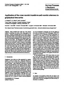
F 2k+2

l k+1

Figure 3.3: The (2,2) motion-compensated LS The resulting motion compensated (2,2) lifting scheme, for a one-level decomposition, is represented in Fig.3.3. Let us see for completeness the equations of the Haar LS. We have:

hk (p) = x2k+1 (p) − x2k (p + F2k+1 (p)) 1 lk (p) = x2k (p) + hk (p + F2k (p)) 2 This means that the (2, 2) LS needs the double motion information that would be necessary for a MC-ed version of the Haar filter, which requires only Forward MVs. Anyway this motion information is quite redundant and in the following chapter we will see some technique to reduce its cost. Note that the Lifting Scheme in (3.5) is perfectly invertible. The equations of reverse transform can be easily deducted the same way as (3.4) is deducted from (3.3). A second worthy observation is that MC-ed (2, 2) LS is by no means limited to integer precision MVF. Indeed, should motion vectors in (3.5) be fractional, we assume the convention that when p ∈ R2 ,

C HAPTER 3. T EMPORAL F ILTERING

29

then xk (p) is obtained by original data by using a suitable interpolation. This feature is very important because sub-pixel MC can bring in a significant improvement in performances. Of course, it comes at some cost: subpixel Motion Estimation and Compensation are far more complex than integer-pixel versions, as they involve interpolations; moreover, sub-pixel MVs require more resources to be encoded. Usually, bilinear interpolation achieves good results without a great complexity while spline-based interpolation [97] has better results but is more expensive. If the motion estimation is accurate, the motion compensated wavelet transform will generate a low-energy high-frequency subband, as it only contains the information that could not be reconstructed by motion compensation. The low-frequency subband will contain objects with precise positions and clear shapes. So, thanks to motion compensation, we are able to preserve both high coding gain and scalability.

3.4

( N, 0) Filters

Since the papers by Secker and Taubman [76] and by Pesquet-Popescu and Bottreau [66], the MC-ed (2, 2) Lifting Scheme has been largely and successfully applied in WT video coding [76, 54, 66, 5, 103, 62, 77, 78, 29, 96, 100]. Nevertheless, it presents some problems and, indeed, its performances are still worse than those of the H.264 encoder, which, thanks to a large number of subtle optimizations achieve currently the best compression performances and currently is the state of the art in video coding. The main problems of MC-ed (2, 2) filter can be summarized as follows. Firstly, it requires a considerable bit-rate for Motion Vectors. This turns out to be quite larger than what is needed by H.264 for Motion Compensation. Indeed, for L temporal decomposition levels with the (2, 2) LS, ∑iL=1 (2/L) Motion Vectors Fields per frame are needed, instead of just one. Moreover, higher decomposition level Motion Vectors are quite difficult to estimate, as they refer to frames which are very distant in time. This results in wide-dynamics, chaotic Motion Fields, which usually require many resources to be encoded. Moreover, multiple-level, sub-pixel MC-ed temporal filtering is characterized by a large computational complexity, and this could prevent realtime implementation even for the decoder.

3.4 ( N, 0) F ILTERS

30

x 2k−2

x 2k−1

F 2k−1

x 2k

x 2k+1

B 2k−1 F 2k+1

h k−1

x 2k+2

B 2k+1

hk

lk

l k+1

Figure 3.4: The (2,0) motion-compensated LS Lastly, as shown by Konrad in [46], the commonly used MC-ed liftingbased wavelet transforms are not exactly equivalent to the original MCWT, unless the motion fields satisfy two conditions, which are invertibility and additivity. These conditions are very constraining and generally not verified. Thus, the resulting transform is inaccurate, and some errors propagate in the low-pass subbands, reducing the coding gain and causing visible blocking artifacts to appear. For all of these reasons, alternatives to the (2, 2) were proposed in literature. Among them, the so-called ( N, 0) Lifting Schemes [3] appears quite interesting. In general, the ( N, 0) Lifting Schemes can be derived by the corresponding ( N, M ) by removing the Update step (this justifies the name). For example, we derive the (2, 0) lifting scheme from the original (2, 2), by removing the update operator. The analytical expression of MC-ed (2, 0) LS is the following:

hk (p) = x2k+1 (p) − lk (p) = x2k (p)

1 [ x (p + F2k+1 (p)) + x2k+2 (p + B2k+1 (p))] 2 2k (3.7)

C HAPTER 3. T EMPORAL F ILTERING

31

Removing the Update step involves several advantages. First of all, we reduce the MV rate, as we do not need to perform any Motion Compensation at the Update Step: the (2, 0) LS requires only the half the MV needed by the original (2, 2) LS. Indeed, as we can see by comparing from fig. 3.4 (representing the (2, 0) LS) and Fig. 3.3, the new LS does not requires backward and forward MV for even frames. Moreover, as no filtering is performed on the “low frequency” subband, temporal scalability is remarkably improved, as it is highlighted in Section 6.7.2. Third, these filters perfectly correspond to their bankfilter WT counterpart, independently from MVF characteristic, and so they are not affected by the blocking artifacts due to non-invertible and nonadditive motion vectors. Taubman [91] noticed that at deeper levels of temporal decomposition, frames are quite different, and therefore, using a low pass filter as the (2, 2) (even if Motion-Compensated) can result in noticeable blurring of low-pass subband. Nevertheless, he claimed a performance superiority of (2, 2) filters on (2, 0), above all on noisy sequences, and proposed some mixed structure, characterized by the possibility to chose the temporal filter according to the temporal decomposition level, or by some form of adaptive filtering which results in a kind of intermediate filter between (2, 2) and (2, 0). This adaptive scheme should be able to modify the impact of the Prediction Stage accordingly with the input data. Indeed, we saw that at low to medium bit-rate, the (2, 0) LS benefits from lower MV rate, and as usually better performances, above all when the sequence considered has considerable motion and low noise contents. Note that, even if (2, 0) LS gave worse performances than (2, 2), it would be interesting to further investigate it, because it assures a better scalability (see Section 6.7.2) and, because its formulation is so simple, that it allows some theoretical development otherwise impossible (see Sect. 4.5).

3.5

Implementation Issues

So far we have considered the problem of temporal filtering with a single decomposition level. However, remarkable improvements in performances are obtained if more complex decompositions are considered. Further decompositions are obtained by applying the MC-ed LS to temporal subbands. As the high frequency subbands are usually scarcely correlated

32

3.5 I MPLEMENTATION I SSUES

LL

LLL MC−ed Temporal Transform

L MC−ed Temporal Transform

Motion

MC−ed Temporal

Estimation

Transform Input Video Sequence

LLH

Motion Estimation LH Motion Estimation H

Temporal SBs

Figure 3.5: Three-level dyadic decomposition for generic temporal filters

and have low energy content, the LS is applied to the lower subband. This process is commonly repeated for three or four levels, as in the scheme in Fig. 3.5, giving rise to a decomposition tree. This scheme is referred to as dyadic decomposition. Any scheme which is not dyadic is generically called packet decomposition. Dyadic decomposition is the most common choice for images, even though packet decomposition has been proposed in literature [101, 70]. The JPEG2000 standard provides dyadic decomposition as default, but extensions allow generic decomposition trees. In our encoder we will consider only the dyadic decomposition for the temporal stage. This means that only the lower frequency subband will be further decomposed. It is worth noting that, in order to perform multiple temporal decompositions, we need adequate motion information. In fact, all the operations performed in order to obtain the lk and hk sequences must be repeated on the low frequency subband. Namely, we need to perform a new ME on the lk sequence, and then a new filtering stage. This means a sequential architecture of the encoder, and a deep interdependence among subbands, which requires very complex optimization processes, see Fig. 3.5. Here another advantage of ( N, 0) LS is highlighted. Indeed, as the lk sequence is just a subsampled version of the input sequence, different decomposition levels can be obtained with parallel processing from the input sequence. Namely, ME and temporal filtering can be performed independently and parallelly for each level, see Fig. 3.6. This is favourable not only for implementation, but also for the optimization of ME, since MV for each subband can be optimized independently level by level, see Section 4.5.

C HAPTER 3. T EMPORAL F ILTERING Input Video Sequence

33

LL

L 2

2

2

Motion

Motion

Motion

Estimation

Estimation

Estimation

MC−ed Temporal

MC−ed Temporal

MC−ed Temporal

Transform

Transform

Transform

H

LLH

LH

LLL

Temporal SBs

Figure 3.6: Three-level dyadic decomposition for ( N, 0) LS A practical problem in temporal WT implementation is related to memory requirements of time filters. Usually, WT filtering is implemented by loading all the data in memory and then performing WT filtering. In the case of temporal filtering of video, this would require a huge memory and moreover would imply an encoding delay as long as the sequence duration itself. A simple solution to the temporal filtering problem is to crop the input sequence in several short subsequences and than compute temporal WT on them. This allows one to implement temporal filtering at low cost, but introduces important impairments to coding efficiency. Indeed for each short sequence we have to manage some kind of border effects. In particular, in order to perform WT we need to extend in some way the data “beyond the border”. Indeed, if we consider an even-length short sequence, when computing the prediction step on the last frame (that has to be considered as odd, since, conventionally, the first frame has a zero, and then even, index), we need a further even frame. At this end we actually replicate the penultimate frame. This means that this prediction is actually performed by using data of a single frame instead of two. The scan-based approach allows to overcome this problem, by computing the temporal transform as it would be by considering all the video sequence as a whole, i.e. without cropping it in subsequences neither cre-

34

3.5 I MPLEMENTATION I SSUES

ating spurious and unnecessary subsequence borders. Moreover this technique does not requires large memory amounts. Initially proposed to reduce the blocking artifacts in the case of spatial WT [64], this technique has then been adapted to the temporal Motion Compensated WT as well [61, 62]. Figure 3.5 shows the differences between the block-based and the scan-based approach. In 3.5(a),block-based temporal WT is shown. In order to perform a single level of decomposition on 8 frames, these are subdivided into two GOP of 4 frames. Each GOP is independently filtered, but, at this end, we need a symmetrical extension of the sequence, obtained by the replication of border frame. On the contrary, the scan-based approach, shown in Fig. 3.5(b),produces the same coefficients that we would get by transforming all the sequence as a whole, without a huge memory occupation. This is achieved by keeping in memory only data necessary for computing next coefficients.

C HAPTER 3. T EMPORAL F ILTERING

x 2k

x 2k+1

hk

x 2k+2

x 2k+3

hk

35

x 2k+2

x 2k+4

h k+1

lk

h k+2

l k+1

x 2k+5

x 2k+6

x 2k+7

h k+2

l k+2

x 2k+6

h k+3

l k+3

GOP k

GOP k+1

(a)

x 2k

hk

x 2k+1

x 2k+2

hk

lk

x 2k+3

x 2k+4

h k+1

l k+1

x 2k+5

x 2k+6

h k+2

l k+2

x 2k+7

...

h k+3

l k+3

(b)

Figure 3.7: Comparison among block-based and scan-based temporal WT. Arrows represent the required motion vectors and dashed frames are obtained by symmetry.

36

3.5 I MPLEMENTATION I SSUES

Chapter 4 Motion Estimation Issues ,

Πα´ ντα $e˜ι 1 H ERACLITUS

4.1

A Brief Overview of Motion Estimation

Motion Estimation (ME) is a very important step in any video encoder, except for very low complexity schemes. In a very general way, we can say that Motion Estimation is a process which accepts a video sequence as input and produces a description of movement occurred in that video. This motion information has many applications, and Video Compression is just one of them. In particular, in Video Compression, ME is of course necessary in order to perform Motion-Compensated operations, such as Motion-Compensated prediction in the case of hybrid coding schemes, or Motion-Compensated temporal filtering in the case of Wavelet Transform coding. However, several other applications exist in the field of video processing. ME is very important in such fields as Video Segmentation, Video Surveillance, Video Restoration. In segmentation problems, ME helps in recognizing objects, since all pixels belonging to the same object 1 Everything

flows

38

4.1 A B RIEF O VERVIEW OF M OTION E STIMATION

presents coherent motion characteristics [35, 1]. For Video Surveillance application, ME is often considered in its most basic form, that is Motion Detection. In this case the relevant motion information is just the presence of moving objects. In Video Restoration, ME is used in order to perform MC-ed temporal filtering for noise reduction or temporal interpolation [6]. ME algorithms can be classified according to three main characteristics: the motion model, the cost criterion, and the search strategy. Many possible choices exist for each of these items, and it is not possible to define the best one, as this strongly depends on applications, and, very often, on input data. In the following, we review shortly some of the most common choices for these three aspects of ME algorithms. A first model is the global motion model, which provides just a single motion information for each frame. This model is extremely simple, but it is well fitted to describe some very common situations such as camera panning on fixed background. Of course, this model is also very cheap in terms of coding resources needed by motion information: we need just one Motion Vector (MV) (that is two scalar parameters) per frame. The model can be made slightly more complex by introducing an affine transformation (i.e. including zoom and rotation) instead of a simple translation. In this case we have six motion parameters per frame. The global motion model is very simple and is able to catch a substantial amount of motion in a generic video sequence. However, in order to achieve a better representation of motion, it is often used together with more complex models, e.g. global motion and block-based motion, or global motion and object motion. The previous model fails when several objects are present in the scene. A straightforward extension is the block based motion model, where each frame is decomposed in rectangular blocks of pixels, and each block is treated as frames were treated in the previous case. This means that for each block we can consider simple movements such as rigid translations, or more complex ones, as affine transformations. The most common approach provides just a translation vector for each block. It is worth noting that the block size can be fixed for the whole frame (this is the motion model compatible with the MPEG-1 and 2 syntax [36, 37]) or it can change, allowing to adaptively describe the motion, according to its local characteristics (the H.264 standard syntax [75, 105] allows variable sized blocks). Despite its simplicity, translational block-based ME (BBME) is quite effective, and is therefore the most common ME technique. Nevertheless,

C HAPTER 4. M OTION E STIMATION I SSUES

39

the affine model is also used sometimes. It is quite more complex than the translational model, but it is able to correctly catch zooms and rotations. On the other hand, it requires the transmission of three times more parameters than the previous method, so it turns out to be quite expensive in terms of both computational complexity and coding rate. Another common model is based on meshes. A mesh is used to cover the frame. The model provides a motion vector (two scalar parameters) per mesh vertex, while the motion vectors for other points are obtained by a suitable interpolation, that is, a bilinear interpolation for rectangular meshes, and an affine interpolation in the case of triangular meshes. The mesh motion model is supported by the MPEG-4 syntax [38, 65] and used in some recently proposed video encoders [79]. Finally, we cite object-based models and Dense Motion Vector Fields. The first model provides a subdivision of video sequence into moving objects: the motion information amounts then to the motion parameters for each object. In the dense MVF case, a vector is provided for each pixel. This is the most general model, as any of the previous ones can be described by a dense MVF. The main problem of dense MVF is they can require a huge amount of resources to be encoded, leaving a meagre budget for coefficient coding. Nevertheless, this approach has some interesting properties, and has been envisaged in scientific literature [85, 67]. We will describe some dense MVF coding technique in Section 5.6. A representation of these motion models is given in Fig. 4.1. The choice of a specific motion model involves a trade-off between accuracy of motion description on a hand and coding cost, computational and implementation complexity on the other. The best option strongly depends on application and data, but, as previously mentioned, translational BBME is the most common motion model for ME. In our work we mainly used this approach, which jointly presents reasonable complexity and good performances, and is quite robust with respect to input data. In the rest of this Section, for the sake of simplicity, we will mainly refer to BBME, but our considerations apply to the other motion models as well. The second classification criterion for ME techniques is the cost function. The estimation process is carried out by searching for motion parameters minimizing a given cost function, which usually represents a distance measure (a metric) between the Motion-Compensated version of the current frame or block and some reference frame or block. In Section 4.2 we will describe in detail some of the most common ME criterion, like

40

4.1 A B RIEF O VERVIEW OF M OTION E STIMATION

(a)

(b)

(c)

(d)

Figure 4.1: Schematic representation of motion models: (a) global motion; (b) block based; (c) dense MVF; (d) object based.

C HAPTER 4. M OTION E STIMATION I SSUES

41

the Sum of Squared Differences (SSD) between current and reference data, and a variation of it. We remark that the SSD criterion is equivalent to the Mean Square Error (MSE). Another very common criterion is based on the Sum of Absolute Differences (SAD) which is simpler to compute and more robust in the presence of outliers. Of course, these are only some of the possible approaches and not necessarily the best ones. In Section 4.5 we will study the problem of optimal ME criterion in the case of WT video coding. The third classification parameter for ME algorithms is the search strategy. Once the motion model and the optimal criterion are established, we have to decide how to find out the motion parameters. For the block based motion model, Block Matching (BM) approach appears to be the most natural choice: the current block is compared with a suitably (i.e. accordingly to the motion model) transformed version of a block of the reference frame. The cost function for this couple of blocks is computed and we choose the motion parameters which minimize this cost. If we control all the possible MV and chose the best one, it is said that an Exhaustive Search has been performed. This is the most computationally demanding method, but of course the one that gives the best results. However, the computational burden of Exhaustive Search can be unacceptable for some applications, like real-time video or streaming on low-power devices. For this reason, sub-optimal search strategies for Block-Matching have been proposed in literature, like the the Log-Search, (sometimes called ThreeStep Search), and the Diamond Search [44]. These techniques usually allow a remarkable complexity reduction without impairing too much motion information accuracy. In our work we used mainly full search ME techniques, as computational complexity was not a major issue in our research. Three-Step search was considered as well, since it has good performances, little computational cost and it provides a progressive description of Motion Vectors. Besides Block Matching, other methods have been proposed in literature, as Phase Correlation [94], Optical Flow, and Statistical (MAP Estimation) methods [85]. Several other parameters have to be set when choosing a ME technique. Among them, we have the block size, the search area and the precision. Let us spend a few words to describe the impact of different precisions on a ME algorithm. The first ME algorithms considered only integer component MVs, but this is actually a tight constrain for the movement of video

42

4.1 A B RIEF O VERVIEW OF M OTION E STIMATION

objects. In fact, objects move independently from the spatial subsampling grid of a video frame, and this calls for sub-pixel Motion Vectors. They can be computed by suitably interpolating the original video sequence and applying the full-pixel ME algorithm on the increased-resolution images. Sub-pixel Motion Compensation is then obtained using the interpolated images instead of the original. It has been early recognized that sub-pixel ME and MC can improve significatively the performances of a video encoder [31], and, therefore, they have been included in all video coding standards from MPEG-2 on. MPEG-2 uses a simple bilinear interpolation for half pixel accuracy ME and MC. The most recent standard H.264 uses a 6-tap filter for half pixel accuracy and a further bilinear interpolation to reach quarter pixel accuracy. Of course, sub-pixel accuracy is more demanding in terms of computational power then full-pixel accuracy that, in turn, is already one of the most complex parts of a generic video encoder. In conclusion, the choice of operational values for all the considered parameters (block size, search area, precision) involves a trade-off between accuracy on a hand, and complexity and encoding cost on the other. Even when all the ME parameters have been chosen in the best possible way, we are far from being sure that the best Motion Vector Field will be found. Actually, a crucial compromise between accuracy and cost of MV has to be considered. Usually, we look for the MV which minimizes a given criterion: this would be the best MV according to such a criterion, but we might have to spend many resources to encode it. It could happen that a slightly less accurate vector could be encoded at a much lower price, allowing to spare resources for coefficients coding, and thus attaining better overall performances. The vector which allows the best overall performances would be the best one in a rate-distortion sense. This compromise is somehow represented in Fig. 4.2. Here we report the Rate-Distortion curve of Motion Vectors, with the rate needed to encode Motion Vectors (this is the cost) on the abscissas, and the corresponding prediction distortion, expressed in terms of MSE (this is the accuracy) on the ordinates. We can imagine to obtain less accurate vectors by increasing the block-size, by reducing the precision, by introducing some regularization constraints in ME, or even by a lossy encoding of MVs. The Motion Vector Field (MVF) which minimize MSE corresponds to the circled point of the graph, characterized by the best accuracy and the highest cost. Nevertheless, this could prove not to be the the best possible MVF

C HAPTER 4. M OTION E STIMATION I SSUES

43

22 20 18

Prediction Error (MSE)

16 14 12 10 8 6 4 2 0

10

20

30

40 50 60 Motion Rate − kbps

70

80

90

100

Figure 4.2: Possible Behavior of Motion Compensated Prediction Error in Function of Motion Rate in a rate-distortion sense, since we can reduce significantly the MVF rate without too much sacrificing its accuracy, by choosing a point at the left of the first one. If we have a limited amount of coding resources, it is probable that the best operational point is placed somewhere at the left of this extreme point, for example it could be the point marked by a × in this graph. Sections 4.3 and 4.4 are about the quest of this optimal point.

4.2

Block Based Motion Estimation (p)

We introduce here some notation for block handling. Let Bk be a block of size 2 (n × n) in the frame k, centred on pixel p = ( p1 , p2 ). We consider even values for n. Moreover, we define B0n = {−n/2, . . . , n/2 − 1}2 , and (p)

Bk (u, v) = xk ( p1 + u, p2 + v) ∀(u, v) ∈ B0n . To compute our motion vectors, we first need a metric between blocks, 2 Square

blocks are not necessary. They are used here just for the sake of simplicity.

44

4.2 B LOCK B ASED M OTION E STIMATION

d( B1 , B2 ). A common metric is the Mean Square Error (MSE), or equivalently, the Sum of Squared Differences (SSD), defined as: h i2 (p) (q) (p) (q) SSD( Bk , Bh ) = ∑ Bk (u, v) − Bh (u, v) (u,v)∈B0n

The relationship among MSE and SSD is simply: (p)

(q)

MSE( Bk , Bh ) =

1 (p) (q) · SSD( Bk , Bh ) n2

Another common criterion is the Sum of Absolute Differences (SAD): ¯ ¯ ¯ (p) ¯ (p) (q) (q) SAD( Bk , Bh ) = ∑ ¯ Bk (u, v) − Bh (u, v)¯ (u,v)∈B0n

These criteria provide good results as long as the mean intensity in both frames is the roughly same. But in real video shots, intensity may vary between two consecutive frames, in which case these criteria can produce inaccurate motion estimations. To overcome this problem, we use also another criterion, the Zero-mean Normalized Sum of Squared Differences (ZNSSD), as it is robust to affine intensity transformations while remaining easy to compute [100]. In order to define this criterion, let us introduce (p) (p) the zero-normalized version of a block Bk , indicated with B˜ k : 1 (p) (p) B˜ k (u, v) = Bk (u, v) − 2 n

∑

(u,v)∈B0n

(p)

Bk (u, v)

that is the block minus its average value. (p) (q) For two given blocks Bk and Bh the ZNSSD formula is given by:

(p)

(q)

ZNSSD( Bk , Bh ) = h (p)

For a given block Bk block

(p+v) Bh

h i2 (p) (q) ∑(u,v)∈B0n B˜ k (u, v) − B˜ h (u, v) (q) (p) ∑(u,v)∈B0n B˜ k (u, v)2 · ∑(u,v)∈B0n B˜ h (u, v)2

i1/2

in frame k, we look for the best corresponding

in frame h by minimizing the following criterion: ´ ³ (p) (p+v) Jh,k (v) = d Bk , Bh

(4.1)

C HAPTER 4. M OTION E STIMATION I SSUES

45

where d is a metric like SAD, SSD or ZNSSD. We will drop the subscripts from criterion J when this information can be deducted by the context. Finally we can define the estimated vector v∗k→k+1 (p) for pixel p: v∗k→k+1 (p) = arg min Jk,k+1 (v) v ∈W

(4.2)

where W = {−w, . . . , w}2 is the search window for block matching and w is then the maximal allowed search distance. Using the symbols of previous chapter, we can call Fk the vector computed by (4.2). The estimated MVF is then : Fk (q) = v∗k→k+1 (p)

∀q ∈ Bpm

where

Bpm = { p1 − m/2, . . . , p1 + m/2 − 1} ×{ p2 − m/2, . . . , p2 + m/2 − 1} and m ≤ n. For m = n, we have the usual non-overlapped block-matching criterion, while if we set Bpm = {p} we compute a different motion vector for each pixel, i.e. a Dense MVF. The advantage of overlapped blockmatching (m < n) with respect to non-overlapped block-matching is that, at the cost of a slightly increased computational burden, we achieve a smoother (less sensitive to noise) MVF. We will refer to the criterion (4.1) as unconstrained ME, since no particular constraint is imposed on vectors. The MVF we can compute in this way are the best possible with respect to the chosen criterion, but not necessarily the best MVF overall. In other words, we can find a very accurate vector (e.g. the one minimizing the MSE) but it cost could be so high that overall performances suffer rather than take advantage from this motion representation. We can represent this situation as the rightmost (circled) point in Fig. 4.2. In this context, it would be interesting to look for a less precise, but also less expensive motion representation, moving toward the optimal point of the curve in Fig. 4.2. Next two Sections are dedicated to this issue. It is also worth noting that the optimal rate for MVs is also dependent on the global available bit-rate: it is obvious that the optimal bit rate for MVF at 64kbps cannot be the same as at 1Mbps. The relationship between total available bit-rate and optimal motion bit-rate is investigated

46

4.3 C ONSTRAINED M OTION E STIMATION

in chapter 7, where some interesting results are derived in the case of high resolution (that is, high total bit-rate). We performed many experiments in order to better understand which criterion would perform better for the proposed encoder, and which are the best values for several ME parameters such as block-size, search area radius, block overlap. Here we summarize the main results. The two criterion SSD and ZNSSD proved to give almost identical performances in terms of impact on the overall Rate-Distortion performances, with a very small (and for all practical interests negligible) advantage for ZNSSD. On the other hand, SAD confirmed its greater robustness in presence of noise (outliers) with respect to SSD. Considering the higher computational cost of ZNSSD, we mainly used SAD and SSD (MSE) for our codec. As far as block size is concerned, we considered only fixed block size ME. With this settings, it turns out that in most cases a block size of 16 pixels provides the best compromise between cost and accuracy of MVF, at least for total bit-rates less that 1.5Mbps. The optimal value for the search area radius is between 12 and 16 pixel for consecutive frames: larger values would increase computational complexity without giving a remarkable benefit. For more distant frames this value should be increased proportionally to the temporal distance. Finally, block overlap proved to slightly increase performances, but at cost of a complexity increase. Usually, an overlap within 25% of the block size proved to be a good choice.

4.3

Constrained Motion Estimation

When MC-ed (2, 2) LS is used, we need a backward MVF and a forward MVF for each frame (see Fig. 3.3). For the (2, 0) LS, half the MVFs are needed, and namely, a backward and a forward MVF for each even frame (see Fig. 3.4). This side information can grow up to represent a remarkable share of the total bit-rate. Here we have a resource allocation problem: we can use our bit budget to encode the MVFs, but we can also try to have a less accurate description of them, using the spared bits to better encode the WT coefficients. This problem calls for an optimal rate-distortion solution, but it seems quite difficult to take into account MVF encoding and residual encoding at the same time, as the second term depends on the first one. With a different approach, we try to answer this question in chapter 7.

C HAPTER 4. M OTION E STIMATION I SSUES

47

Here we look for some suboptimal solution. An interesting one is what we call Constrained Motion Vectors. We impose some constraints on MVFs that allow us to significantly reduce the rate needed for MVF’s encoding, but, on the other hand, prevent us to achieve the best motion estimation. Initially, we impose a very simple constraint: we want the backward MVF to be the opposite of the forward one. Then we look for a displacement vector, which under this constraint minimizes a quantity depending on both the forward and the backward error, e.g. their sum: v∗ = arg min J (v)

(4.3)

h ³ ´ ³ ´i (p) (p−v) (p) (p+v) J (v) = d Bk , Bk−1 + d Bk , Bk+1

(4.4)

v ∈W

with:

Where d( B1 , B2 ) can be any suitable metric. The advantage of constrained search is that we obtain symmetrical MVF, so we can send just every second MVF, using the spared bit budget to better encode wavelet coefficients [100]. On the other hand, constrained search does not allow us to get the best estimation, except for some specific motion configurations. This reflects the fact that the proposed criterion is based on a very simple model, in which the motion is constant and then Bk = − Fk (i.e. zero acceleration). The effectiveness of this ME criterion is then tightly bounded to the correctness of the zero-acceleration model. If in the considered video sequence motion is regular (i.e. only rarely the acceleration is significant), our model will correctly catch motion information. Otherwise, when acceleration is important, the proposed model will fail and compute suboptimal motion vectors. Nevertheless, their cost will always be less than in the case of unconstrained ME. In order to better understand the trade-off between accurate MVF description and improved wavelet coefficient encoding, some experiments were performed. In the first one we compared our codec performances when the MVFs were estimated with the unconstrained and with the constrained search. The experiments were carried out on the first 64 frames of the sequence “foreman”, with a block size of 16 pixels. The results are shown in figure 4.3(a). Note that the constrained search method requires about half the rate for MVF with respect to the unconstrained method. However, in this

48

4.3 C ONSTRAINED M OTION E STIMATION

120

140 Exhaustive search Constrained search

No Motion Compensation Exhaustive search Constrained search

120

100

60

distortion − MSE

distortion − MSE

100 MVF rate not taken into account Unconstrained: 86.01 kbps Constrained: 39.60 kbps

80

40

MVF rate taken into account Unconstrained: 86.01 kbps Constrained: 39.60 kbps

80 60 40

20

0

20

250

500

750

1000 1250 1500 rate − kbps

(a)

1750

2000

0

250

500

750

1000 1250 1500 rate − kbps

1750

2000

(b)

Figure 4.3: Comparison between ME methods (a) and their impact on codec performances (b)

figure we do not take into account the rate needed for MVF encoding, as we want just to understand how much the worse motion estimation affects motion compensated wavelet transform. The graph shows that the loss is quite small, as the MSE increase varies from 1% to 9%. In order to perform a thorough comparison between the two methods, in figure 4.3(b) we considered also the cost of MVF encoding. Moreover, the performances of the codec without motion compensation were also added. The graph shows that the constrained method has the best performances at low and medium rates, and it is roughly equivalent to unconstrained search method at high rates. These results can be interpreted as follows: the unconstrained MVFs corresponds (for a given set of ME parameters, as block size and precision) to the rightmost point of the curve in Fig. 4.2. When we impose some constraint, we begin to move toward the left in this graph, hopefully towards the optimal point. Indeed, for low-to-medium bit-rates, the constrained MVF gives better overall performances than the unconstrained one, so we are actually getting near the optimal operation point.

C HAPTER 4. M OTION E STIMATION I SSUES

49

Figure 4.4: Irregular motion vector estimation

4.4

Regularized Motion Estimation

In this Section we keep exploring the left part of the curve in Fig. 4.2, with the goal of further decreasing the bit-rate needed by MVF, without degrading too much motion information. We try to achieve this goal by introducing MVF regularization. The basic idea is to impose some reasonable constraints to the ME criterion, in order to get a MVF that can be efficiently encoded and that however remains a good estimation of motion. In previous Section we proposed a simple symmetry constraint, which led to the cost function (4.4). Here we modify the estimation criterion by adding some regularization constraint to the cost function, with the aim of obtaining a more efficiently encodable MVF. Indeed, even though the symmetry constraint implies some smoothing, MVFs estimated by the criterion (4.4) can still suffer from some irregularities: see for example Fig. 4.4, where it is reported an estimated MVF for the “foreman” sequence: in the quite homogeneous helmet area, the MVF, even if minimizes the metric, has a remarkable entropy. The problem is that in a homogeneous area, many motion vectors can have very low and very close values for the cost function. In this case, choosing a suboptimal vector do not significatively increase prediction er-

50

4.4 R EGULARIZED M OTION E STIMATION

Figure 4.5: Regularized motion vector field ror, while can help in reducing MVF entropy. Hence we introduce a couple of new constraints: a length penalty and a spatial variation penalty. The new criterion is expressed as follows: · ¸ ||v||2 ∗ 2 2 v = arg min J (v) + α (4.5) + β(||∇v x || + ||∇vy || ) ||v||2max v ∈W where J (v) is still expressed by (4.4). In a homogeneous area, null or homogeneous vectors are then more likely to be chosen, reducing the occurrence of chaotic regions in the MVF. In Fig.4.5 the resulting MVF is shown. It is clear that the constraints help in regularizing the MVF. Initial experiments showed the existence of values for α and β which allow a fair regularization without degrading too much the motion information. We can gain a deeper insight on this phenomenon by evaluating the effect of regularization on the first order entropy of regularized MVFs and the respective prediction MSE, see Tab.4.1. These results were obtained for the test sequence “foreman”, with a block size of 16 × 16 and whole pixel precision. In this table we also reported the entropy of Wavelet Transformed (3 level dyadic decomposition) MVFs, in order to show that WT allows reducing entropy, and that regularization is even more effective in the wa-

C HAPTER 4. M OTION E STIMATION I SSUES

α

β

0 0 0 10 10 10 30 30 30 100 100 100

0 4 20 0 4 20 0 4 20 0 4 20

Entropy of MVF [bit/vector] 4.33 3.72 3.37 3.93 3.61 3.30 3.81 3.58 3.28 3.62 3.46 3.20

51

Entropy of WT [bit/vector] 0.56 0.35 0.26 0.47 0.34 0.25 0.45 0.34 0.25 0.42 0.33 0.25

Prediction MSE 48.22 49.90 56.54 48.24 49.97 56.44 48.35 50.08 56.54 48.98 50.58 56.91

Table 4.1: Regularization parameters effect

37 36 35

PSNR − dB

34 33 32 31 30 29 28 200

Unconstrained Constrained 400

600

800 rate − kbps

1000

1200

1400

Figure 4.6: Impact of ME methods on codec performances

52

4.5 O PTIMAL ME

FOR

WT- BASED V IDEO C ODING

velet domain. This results suggest us to look for an encoding technique that makes use of WT of regularized MVFs, like the one described in Section 5.6. We also remark that with a suitable choice of parameters, we can achieve an entropy reduction of 16% (and even 40% in WT domain), while the prediction MSE increases only of 1.5%. It is of course necessary to evaluate the impact of constrained ME on the whole video coder. So, in Fig.4.6 we compared global RD performances of our video coder when the usual unconstrained ME and the proposed constrained ME criteria are used. These results were obtained on the “foreman” sequence, with regularization parameters α = 10 and β = 5, precision of whole pixel, and block size of 16 × 16. The graph shows that the proposed method yields globally better performances, especially at low to medium rates, where we achieve up to 1.3 dB of improvement with respect to the usual unconstrained technique. This result confirm the intuitive idea that at low rates it is better to have an approximate but cheap description (in term of needed encoding resources) of motion and to dedicate more resources to transform coefficients. This technique allows us to get a bit closer to the optimal point of Fig. 4.2.

4.5

Optimal ME for WT-based Video Coding

In this Section, we try to analyze the problem of optimal Motion Estimation in the framework of wavelet video coding. As mentioned above, Motion Compensation is of crucial importance in order to obtain good performances in video coding, be it the classical hybrid coding or the newer wavelet-based algorithms. A good ME is equally very important. Nevertheless, the criterion for ME that is usually employed is the minimization of MSE (or related metrics) between reference and predicted (Motion Compensated) frames. This approach is optimal as far as hybrid coding is concerned, but this is not necessarily true for a generic Wavelet Video Coder. In this case, a deeper analysis is needed, since we are no longer coding the prediction error, but the transform coefficients, so minimizing the error energy could not be the best approach anymore. The need of an optimal approach to ME for wavelet video was early recognized by Choi and Woods [21]. They asserted that while for hybrid coders the objective of motion estimation is to minimize the mean squared

C HAPTER 4. M OTION E STIMATION I SSUES

53

prediction error, for MC-ed temporal analysis, the objective should be changed to maximization of the Coding Gain (CG). As the filter they used for Temporal Analysis (Haar filter) is orthogonal, the CG is expressed as the ratio of the arithmetic and geometric means of subband variances. The maximum CG is nearly achieved by minimizing the energy (variance) of the temporal high frequency subband, since the variance of the temporal low frequency subband is relatively constant. Using the Haar filter for Temporal Analysis, the temporal high frequency subband is just a scaled version of the prediction error signal. Thus, the minimization of MSE turns to be nearly optimal in their case. Nevertheless, when a generic temporal filter is used, a further analysis is needed. Here, indeed, we want to analyze the problem of optimal ME for MC-ed Lifting Scheme video coders in a more general way. We will use a general approach as far as possible, then we will turn to ( N, 0) filters, which allow a deeper analysis, and even an analytical solution of the optimal ME criterion problem.

4.5.1

Notation

Let us now define a few notations in order to manage MVs related to multiple decomposition levels. As usual, we use vk→h (p) to refer to the displacement that the pixel p in frame k will have in frame h. The k-th (0) frame of input sequence is referred to as xk (p). We indicate with hk (p) (1)

the first high frequency (H) temporal subband sequence, with hk (p) the second high frequency (LH) subband sequence, and so on. Analogously (0) (1) lk (p), lk (p) are the low frequency subband sequences. We consider L levels of dyadic temporal decomposition, resulting in M = L + 1 temporal subbands; we indicate with v(0) the set of all motion vectors needed to compute the first temporal decomposition from the input sequence, and in general, with v(i) the set of vectors needed to compute the (i + 1)-th temporal decomposition from the previous level. These vectors are shown in Fig. 4.7 for the case of (2, 2) LS and two levels of temporal decomposition. We see that in this case v(0) is made up of all vectors vk→k+1 and vk+1→k for all k, while v(1) is constituted by vectors v2k→2k+2 and v2k+2→2k for all (1) k. It is clear moreover that in order to compute each frame of hk we need all vectors of the sets v(0) and v(1) .

54

4.5 O PTIMAL ME 0

1

2

3

4

FOR 5

WT- BASED V IDEO C ODING 6

7

8

x h(0)

v(0)

l (0) h(1)

v(1)

l (1)

Figure 4.7: Scheme of a two-levels temporal decomposition with the (2, 2) LS. In this case V1 = {v(0) , v(1) }. More in general, in order to compute a single level of temporal decomposition with a ( N, M ) LS we need N vectors per frame for the high frequency subband and M vectors per frame for the low frequency subband. Let us call Vi the set of all vectors necessary to compute the i-th decomposition level. In general, we need all the vectors from previous de(i ) composition levels in order to compute hk , i.e., Vi = {v(0) , v(1) , . . . , v(i) }. This means that in the general case, as far as motion vectors are concerned, all SBs depend on one another.

4.5.2

Optimal Criterion

ME is used in order to find MVs that describe displacement of objects from a frame to another. The optimality criterion in subband coding is the maximization of the Coding Gain [30, 21], which is defined (see chapter 1 as well) as the ratio among DPCM (the distortion of scalar quantization, i.e. ∗ (the minimum distortion achievPCM coding, of input signal) and DTC able by Transform Coding). The optimal ME criterion should maximize the CG instead of minimizing the MSE of prediction error. In particular, DPCM does not depend on Motion Compensation, since it refers to the input, i.e. non-transformed, signal. Therefore we can focus on minimization ∗ . of DTC ∗ for generic WT coding We show in Appendix A how to express DTC

C HAPTER 4. M OTION E STIMATION I SSUES

55

with M subbands, see Eq. (A.11). Let M be the number of subbands, Ni the number of coefficients of band i, N the total number of WT coefficients, and ai = Ni /N. We have: ¯

∗ DTC = W Hρ2 2−2b

(4.6)

where b¯ is the available bit rate in bpp and: M

W=

i =1 M

H= ρ2 =

a

∏ wi i a

∏ hi i i =1 M ³

∏ i =1

σi2

´ ai

(4.7)

Here, wi is a weight accounting for possible non-orthogonality of WT filters, see section 6.4; hi is the subband shape factor, see Eq. (A.3). We should consider three-dimensional (i.e. spatiotemporal) SBs, but actually we will consider only temporal SBs. Indeed, some earlier studies on this problem showed that considering spatiotemporal SBs instead of temporal SBs gives little or no gain [21]. We observe that W and b¯ do not depend on motion vectors; moreover, we make the hypothesis that the shapes of subband pdfs do not depend on MV either. In this case all the hi and H are not affected by ME. This means that the optimal ME strategy should be the minimization of ρ2 , that is a kind of weighted geometric mean of temporal subband variances; as a matter of fact, it would coincide with the geometrical mean of subband variances if ai = 1/M and wi = 1 ∀i ∈ {1, 2, ..., M }: this happens in the case of orthogonal subband coding. Unfortunately, in the general case, the minimization of ρ2 is not an easy task. This problem is quite complex because motion vectors related to the i-th decomposition level affect all subbands {i, i + 1, . . . , M }. This means that we cannot simply chose v(i) such that σi2 is minimized, as this set of vectors influences higher frequency subband variances as well. Therefore, in the general case, this problem calls for a joint optimization of motion vectors of all levels in order to minimize (4.7).

56

4.5 O PTIMAL ME 0

1

2

3

4

FOR 5

WT- BASED V IDEO C ODING 6

7

8

x h(0)

v(0)

l (0) h(1)

v(1)

l (1)

Figure 4.8: Scheme of a two-levels temporal decomposition with the (2, 0) (1)

LS. In this case V1 = {v(1) }, as hk is computed directly from xk indepen(0)

dently from hk

The joint optimization problem is difficult to approach analytically and extremely demanding in terms of computational power. But, with a suitable choice of temporal filters, it is possible to simplify it remarkably. In particular, we consider the class of ( N, 0) LS. In this case, the low pass output of WT is just the input sequence with temporal subsampling, then it does not depend on motion vectors. Another crucial consequence is that the i-th high frequency subband is computed directly from the input sequence, independently from other SBs. An example is shown in Fig. 4.8, for the (2, 0) LS and two level of tem(1) poral decomposition. We see that we can compute hk directly from the input sequence and from the vectors v(1) . More in general, as we com(i ) ( i −1) pute hk from lk which in turn is just the input sequence undersami pled by a factor 2 , this subband depends only on v(i) instead of all the v(0) , v(1) , . . . , v(i) . This means also that all the subband variances are actually independent of one another, and that they can be minimized separately. In other words, each v(i) can be optimized separately, providing that it minimizes the i-th high frequency SB variance. The optimal ME for a ( N, 0) LS has to estimate v(i) which is the trajectory of current pixel in a subset of frame centred on current frame, and made up of N + 1 frames of the original sequence subsampled with a factor 2i .

C HAPTER 4. M OTION E STIMATION I SSUES

57

As the optimization is carried out in the same way for each decomposition level, we will refer from now on to the first one, and will drop the superscript from hk for the sake of simplicity.

4.5.3

Developing the Criterion for a Special Case

Further analytical developments are possible if we refer to a specific ( N, 0) LS as the (2, 0). Let us recall the equation for this special case.

hk (p) = x2k+1 (p) −

1 [ x (p + v2k+1→2k (p)) + x2k+2 (p + v2k+1→2k+2 (p))] 2 2k

lk (p) = x2k (p) This mean that, in this case, the trajectory v(0) for the frame 2k and for the first decomposition level is just a couple of vectors: v(0) = {v2k+1→2k , v2k+1→2k+2 } This expression can be generalized to the i-th decomposition level: n o v(i) = v2i−1 (2k+1)→2i−1 2k , v2i−1 (2k+1)→2i−1 (2k+2) The optimal trajectory v(i)∗ is the one minimizing the high frequency band variance. Since this subband has zero mean, this is equivalent to minimize its energy. We can refer to the first high frequency subband without losing generality as for the other band it suffices to refer to the suitably subsampled version of the input sequence. For the high frequency subband, we can simplify the notation of the lifting scheme as follows: hk (p) = x2k+1 (p) −

1 [ x (p + F2k+1 (p)) + x2k+2 (p + B2k+1 (p))] 2 2k

lk (p) = x2k (p) where Bk = vk→k−1 and Fk = vk→k+1 as usual. The optimal trajectory is given by: v(0)∗ = arg min E {hk (p)} B2k+1 ,F2k+1

58

4.5 O PTIMAL ME

FOR

WT- BASED V IDEO C ODING

Where we have: hk (p) = x2k+1 (p) −

1 [ x (p + F2k+1 (p)) + x2k+2 (p + B2k+1 (p))] 2 2k

1 (p) − x2k (p + F2k+1 (p))+ [x 2 2k+1 x2k+1 (p) − x2k+2 (p + B2k+1 (p))] 1 = (eF + eB ) 2

=

and e F [eB ] is the forward [backward] motion-compensated prediction error: e F = x2k+1 (p) − x2k (p + F2k+1 (p)) eB = x2k+1 (p) − x2k+2 (p + B2k+1 (p)) This means that the optimal trajectory minimizes the energy of the sum of this errors. Further developing, we have to minimize: 1 E (eB + eF ) 2 1 1 = E (eB ) + E (e F ) + heB , e F i 2 2

E [hk (p)] =

In conclusion: ∗ ∗ B2k +1 , F2k+1

·

= arg

min

B2k+1 ,F2k+1

1 1 E (eB ) + E (eF ) + heB , eF i 2 2

¸ (4.8)

Equation (4.8) is what we need in order to compare the optimal ME criterion to the usual MSE based criterion. With the usual MSE based criterion, we independently minimize E (eB ) and E (e F ), so we probably attain a low value of the optimal criterion but not necessarily the minimum, as we do not take into account the mixed term. This term grows larger when the two errors images are more similar. This means that the optimal backward and forward vector are not independent as they should produce error images as much different as possible, being not enough to barely minimize error images energies. In other words, regions affected by a positive backward error, should have a negative forward error and viceversa.

Chapter 5 Motion Vector Encoding

There are more things in heaven and earth, Horatio, than are dreamt of in your philosophy. W ILLIAM S HEAKSPEARE Hamlet, prince of Denmark, 1601

This chapter summarizes main results obtained in Motion Vector Field (MVF) coding with JPEG2000-based techniques. Motion information obtained by a generic ME algorithm are usually highly redundant, so, in order to obtain an efficient coding, the Motion Vectors have to be compressed. In the previous chapter we saw several techniques for changing MV entropy directly at the ME stage. Afterward, MV are supposed to be losslessly encoded and transmitted to the receiver, and, indeed, lossless methods are the object of the first and largest part of this chapter. However, an alternative approach is considered in Section 5.6, in which we perform ME without caring for MV rate, that is we look for the most accurate motion information, but then consider lossy MV coding techniques. Another issue we considered in MV encoding was compatibility with JPEG2000 standard. Since our target is to implement a video encoder with the highest possible compatibility with this standard, we felt that also MVs should be encoded by means of JPEG2000. Of course, as this is a still image coding algorithm, we cannot expect to provide the best possible

60

5.1 M OTION V ECTOR D ISTRIBUTION

performances, but this appears to be compensated for by the compatibility with the standard. Before describing the techniques for MV encoding, we present a first section where some statistics of MVs are given and analyzed. Then our techniques are described, together with experimental results. We tested proposed techniques in many different configurations, in order to better understand their potential performances. Therefore, several sequences were considered, and Motion Estimation precision and block size were changed in order to investigate the influence of these parameters on vector coding.

5.1

Motion Vector Distribution

We evaluated the distribution of Motion Vector Fields in the sequences “flowers and garden” (250 frames),“bus” (150 frames), and “foreman” (300 frames). All these sequences have a relevant motion content, but in the first one, motion is pretty regular, in the second one, it is regular but complex, as many moving objects appear on the scene, and in the third one, motion is quite chaotic. Full pixel and half pixel precisions were considered. In figures from 5.1 to 5.6, backward and forward vectors for the first three temporal decomposition levels are shown. The log10 of relative frequency is reported, with null vector frequency situated at image center. We remark that for successive temporal levels the search area increases, since temporally distant frames can involve wide movements. This results in a more spread MV distribution at higher temporal levels. Anyway, the distributions show a good regularity, and are pretty concentrated around the null vector. This comes from regularization techniques, which tend to assign a null vector when estimation is not accurate. From the analysis of these distributions, we can get information on motion content of the sequences and some hint about how to encode this Motion Vectors. Figures 5.1 and 5.2 shows that motion in the “flowers and garden” sequence is quite regular, with a dominant horizontal motion toward the left direction. This sequence is actually a camera panning on an almost statical background. From Fig. 5.3 and 5.4 we can deduce that in the “bus” sequence motion

C HAPTER 5. M OTION V ECTOR E NCODING

61

is more complex, even though we have mainly horizontal movements. Indeed, in this sequence we have an horizontal camera panning on a bus and moving cars. The “foreman” sequence is characterized by a more complex motion, as it appears from Fig. 5.5 and 5.6. Many null vectors are estimated, but the distribution exhibits several secondary peaks, coming from different movements of the objects and of the camera in this sequence. By analyzing these distributions and by taking a look to the video sequences themselves, we can conclude that MVFs for these sequences are quite spatially correlated, but can present relevant temporal variations. We note also that the distributions have often high values on the axes, i.e. many vectors with a single null component are estimated. As the ME algorithm we use does not allow vectors pointing outside the frame, the estimation of vectors near the border of the image has often a null value for the component orthogonal to the border, see an example in Fig. 5.7 (left).

5.2

Encoding Techniques: Space Compression

We have proposed, implemented and tested some methods to encode Motion Vectors with JPEG2000 algorithm. The basic idea is that motion vector fields exhibit a remarkable spatial correlation, that has to be reduced in order to achieve compression. A still image compression algorithm would accomplish the job, and so JPEG2000 is used. Of course, it has to be adapted to these peculiar data and to our requirements. Therefore, we used the following general settings for the JPEG2000 encoder: • no wavelet decomposition (0 decomposition levels); • no psychovisual weighting of components; • all bitplane encoded. This configuration assures reversible (lossless) coding, as, indeed we use the EBCOT encoder on MV data. Anyway, there are several way to arrange the data before sending them to the encoder. In this section, we consider three simple encoding strategies, trying to take advantage from spatial correlation of MV. We choose to not perform wavelet decomposition since this operation proved to increase the encoding cost for the lossless case.

62

5.2 E NCODING T ECHNIQUES : S PACE C OMPRESSION

Backward MVF Distribution − Level 1 −16

Forward MVF Distribution − Level 1 −16 −1

−8

−1 −8

−2 0

−3 −4

8

−2 0

−3 −4

8

−5 16 −16

−8

0

8

−5 16 −16

16

−8

(a)

0

8

16

(b)

Backward MVF Distribution − Level 2 −32

Forward MVF Distribution − Level 2 −32 −1

−1 −16

−16 −2

−2 0

−3

16

32 −32

−16

0

16

0

−3

−4

16

−5

32 −32

32

−4 −5 −16

(c)

0

16

32

(d)

Backward MVF Distribution − Level 3 −64

Forward MVF Distribution − Level 3 −64 −1

−1 −32

−32 −2

−2 0

0

−3

−3 32

64 −64

−4

−32

0

(e)

32

64

−5

32

64 −64

−4

−32

0

32

64

−5

(f)

Figure 5.1: MVF Distributions: “flowers and garden”, full pixel precision

C HAPTER 5. M OTION V ECTOR E NCODING

Backward MVF Distribution − Level 1 −16

63

Forward MVF Distribution − Level 1 −16 −1

−8

−1 −8

−2 0

−3 −4

8

−2 0

−3 −4

8

−5 16 −16

−8

0

8

16 −16

16

−5 −8

(a)

0

8

16

(b)

Backward MVF Distribution − Level 2 −32

Forward MVF Distribution − Level 2 −32 −1

−16

−1 −16

−2 0

−3

16

−4

32 −32

−5 −16

0

16

32

−2 0

−3

16

−4

32 −32

−5 −16

(c)

0

16

32

(d)

Backward MVF Distribution − Level 3 −64

Forward MVF Distribution − Level 3 −64 −1

−32

−2

−1 −32

−2

0

−3

0

−3

32

−4

32

−4

64 −64

−5 −32

0

(e)

32

64

64 −64

−5 −32

0

32

64

(f)

Figure 5.2: MVF Distributions: “flowers and garden”, half pixel

64

5.2 E NCODING T ECHNIQUES : S PACE C OMPRESSION

Backward MVF Distribution − Level 1 −16

Forward MVF Distribution − Level 1 −16 −1

−8

−1 −8

−2 0

−2 0

−3 8

16 −16

−4

−8

0

8

−3 8

−4

16 −16

16

−8

0

(a)

8

16

(b)

Backward MVF Distribution − Level 2 −32

Forward MVF Distribution − Level 2 −1

−32 −1

−1.5 −16

−2

−1.5

−16

−2

−2.5 0

−3

−2.5

0

−3

−3.5 16

−4

−3.5

16

−4

−4.5 32 −32

−16

0

16

32 −32

32

−4.5 −16

0

(c)

16

32

(d)

Backward MVF Distribution − Level 3 −64

Forward MVF Distribution − Level 3 −64 −1.5 −2

−32

−1.5 −2

−32

−2.5 −3

0

−2.5 0

−3

−3.5 32

−4

−3.5 32

−4

−4.5 64 −64

−32

0

32

(e)

64

64 −64

−4.5 −32

0

32

(f)

Figure 5.3: MVF Distributions: “bus”, full pixel

64

C HAPTER 5. M OTION V ECTOR E NCODING

Backward MVF Distribution − Level 1 −16

65

Forward MVF Distribution − Level 1 −16 −1 −1.5

−8

−1 −1.5

−8

−2 −2.5

0

−3

−2 −2.5

0

−3

−3.5 8

−4

−3.5 8

−4

−4.5 16 −16

−8

0

8

−4.5 16 −16

16

−8

0

(a)

8

16

(b)

Backward MVF Distribution − Level 2 −32

Forward MVF Distribution − Level 2 −1

−32

−1

−1.5 −16

−2

−1.5 −16

−2

−2.5 0

−3

−2.5 0

−3

−3.5 16

−4

−3.5 16

−4

−4.5 32 −32

−16

0

16

−4.5 32 −32

32

−16

0

(c)

16

32

(d)

Backward MVF Distribution − Level 3 −64

Forward MVF Distribution − Level 3 −64 −2

−2 −32

−2.5

−32

−2.5

−3 0

−3.5 −4

32

−3 0

−3.5 −4

32

−4.5 64 −64

−5 −32

0

32

(e)

64

−4.5 64 −64

−5 −32

0

32

(f)

Figure 5.4: MVF Distributions: “bus”, half pixel

64

66

5.2 E NCODING T ECHNIQUES : S PACE C OMPRESSION

Backward MVF Distribution − Level 1 −16

Forward MVF Distribution − Level 1 −16 −1

−1 −8

−2 −3

0

−8

−2 −3

0

−4 8

−4 8

−5 16 −16

−8

0

8

−5 16 −16

16

−8

(a)

0

8

16

(b)

Backward MVF Distribution − Level 2 −32

Forward MVF Distribution − Level 2 −32 −1

−1 −16

−2

0

−3 −4

16

−16

−2

0

−3 −4

16

−5 32 −32

−16

0

16

−5 32 −32

32

−16

(c)

0

16

32

(d)

Backward MVF Distribution − Level 3 −64

Forward MVF Distribution − Level 3 −1

−64

−1

−32

−2

−32

−2

0

−3

0

−3

32

−4

32

−4

64 −64

−5 −32

0

(e)

32

64

64 −64

−5 −32

0

32

(f)

Figure 5.5: MVF Distributions: “foreman”, full pixel

64

C HAPTER 5. M OTION V ECTOR E NCODING

Backward MVF Distribution − Level 1 −16

67

Forward MVF Distribution − Level 1 −16 −1

−1 −8

−2 −3

0

−8

−2 −3

0

−4 8

−4 8

−5 16 −16

−8

0

8

−5 16 −16

16

−8

0

(a)

8

16

(b)

Backward MVF Distribution − Level 2 −32

Forward MVF Distribution − Level 2 −1

−32

−1

−16

−2

−16

−2

0

−3

0

−3

−4

16

−4

16

−5

−5 32 −32

−16

0

16

32 −32

32

−16

0

(c)

16

32

(d)

Backward MVF Distribution − Level 3 −64

Forward MVF Distribution − Level 3 −64 −1.5

−1.5 −2

−32

−2

−32

−2.5

−2.5 −3

0

−3

0

−3.5

−3.5 −4

32

−4.5

−4

32

−4.5

−5 64 −64

−32

0

32

(e)

64

−5 64 −64

−32

0

32

(f)

Figure 5.6: MVF Distributions: “foreman”, half pixel

64

68

5.2 E NCODING T ECHNIQUES : S PACE C OMPRESSION 12 10 8 6 4 2 0 −2 3 2 1 0 −1 −2 −3

Figure 5.7: Example of MVF and corresponding images for the JP2K Single Image technique The first strategy is the most straightforward: we consider the horizontal and vertical component of a MVF as a couple of images, and the two resulting files feed as two input components the JPEG2000 encoder, which outputs the encoded stream and the lossless encoding rate. This is repeated for each MVF. An example is shown in Fig. 5.7, where we report a MVF for the “flowers” sequence, and the corresponding couple of images. We note that these images are scaled by the block size with respect to the video frames (as a “pixel” is obtained for each block), so the larger the blocks, the smaller these MVF images. We refer to this first strategy as JP2K Single Image. The second strategy aims avoiding the problem of managing too small images, that is what can happen with the first strategy. Let N be the number of MVFs; the horizontal components of all MVFs are pasted together in a large image, made up of M1 × M2 MVFs where N = M1 · M2 . The same is done for the N vertical components. Then the two images are given in input to the encoder, as two components of a single image. An example of these MV images is given in Fig. 5.8, where we show a couple of images taken from the “flowers and garden” sequence. This example shows how these images can be in fact quite regular, and so we can expect pretty good performances if motion is regular. We refer to this strategy as JP2K Big Image.

C HAPTER 5. M OTION V ECTOR E NCODING

(a)

69

(b)

Figure 5.8: Example of MVF images for the JP2K Big Image technique: horizontal (a) and vertical (b) components. Third strategy: each vector field gives two components images, as in Fig. 5.7. All of these images in a group of pictures (GOP) are regarded as components in a multi-component image, and jointly encoded. We refer to this last technique as JP2K Spectral.

5.2.1

Experimental Results

We considered the following test sets: we encoded MVFs computed on the first 64 frames of the gray-level ”foreman” sequence, with full and half pixel precision, and block sizes 8 × 8 and 16 × 16. The MVs have been computed with a block matching algorithm, which minimizes a MSE based criterion, with a slight regularization (i.e. low values of α and β, see Section 4.4). Up to three temporal decomposition levels have been considered, and results are provided for each of them. Indeed, as we saw in previous Section, MV belonging to different decomposition levels can have quite different characteristics: firstly the dynamics increases with the level; moreover, at increasing levels, ME involves frames which are quite distant in time, and then can be quite different. This means that estimated vectors for these levels can be irregular and chaotic, in other word, difficult to encode. This will be confirmed by the increase in entropy of MV, as observed in this test. In order to assess the effectiveness of the proposed strategies, we com-

70

5.2 E NCODING T ECHNIQUES : S PACE C OMPRESSION

Method

No. of Time Dec. Levels 1 2 3

Joint Entropy Differential Entropy

4.27 4.53

4.61 4.98

4.93 5.35

JP2K Single Image JP2K Big Image JP2K Spectral

4.86 4.32 4.71

5.34 4.61 5.15

5.86 4.91 5.55

Table 5.1: Experimental results: full pixel precision, block size 8 × 8 Method

No. of Time Dec. Levels 1 2 3

Joint Entropy Differential Entropy

3.33 3.44

3.61 3.83

3.86 3.99

JP2K Single Image JP2K Big Image JP2K Spectral

5.69 3.55 3.81

6.15 3.92 4.28

6.64 4.25 4.80

Table 5.2: Experimental results: full pixel precision, block size 16 × 16 pared the coding cost to the first order entropy of MVFs, called here “Joint Entropy” in order to emphasize that we are considering the vectors components jointly. Further on we will consider the component Marginal Entropy as well. Moreover, for this test, we also computed the entropy of the differences between each MVF and the previous one. This entropy value represents a lower bound for a temporal predictive encoding technique. We compute this quantity in order to assess wether such a strategy could be favourable. The results of our tests are synthesized in Tab. 5.1 to 5.4. In these tables, we report the encoding cost per vector expressed in terms of bits needed for encoding a single vector. The entropy is expressed in bits per vector as well. Bold types are used for the lowest value for a specific decomposition level. Italic types are used for the best encoding technique. From these results we can draw some conclusion. • Differential Entropy is always larger than Joint Entropy. This suggest

C HAPTER 5. M OTION V ECTOR E NCODING

Method

71

No. of Time Dec. Levels 1 2 3

Joint Entropy Differential Entropy

4.90 5.14

5.18 5.51

5.43 5.81

JP2K Single Image JP2K Big Image JP2K Spectral

5.83 5.35 5.69

6.30 5.63 6.13

6.77 5.86 6.48

Table 5.3: Experimental results: half pixel precision, block size 8 × 8 Method

No. of Time Dec. Levels 1 2 3

Joint Entropy Differential Entropy

4.23 4.29

4.46 4.63

4.66 4.87

JP2K Single Image JP2K Big Image JP2K Spectral

6.98 4.88 5.10

7.46 5.25 5.60

7.92 5.52 6.09

Table 5.4: Experimental results: half pixel precision, block size 16 × 16 us that differential coding techniques are not well suited for MV encoding. Moreover, as we expected, Entropy increases with temporal decomposition levels. • The first JPEG2000 strategy (JP2K Single Image) has the worst performances, as it has to compress quite small images, with peculiar dynamics. Indeed, it performs especially badly when bigger blocks (i.e. smaller MVF images) are considered. Moreover it performs badly with full pixel and sub-pixel precisions. • The JP2K Big Image strategy has coding cost close to the entropy when small blocks with full pixel precision are considered, as in this case we have bigger and more correlate MVF images. In one case JP2K Big Image has a coding cost lower than the Joint Entropy. This is not surprising, as we consider a first order Entropy, while the EBCOT coding technique takes advantage of contextual information

72

5.3 E NCODING T ECHNIQUES : T IME C OMPRESSION [90]. In any case it is always better than the other techniques. • The JP2K Spectral strategy performs worse than the JP2K Big Image. A possible explanation is the small dimensions of each component, that is in this case, only 19 × 22 pixels. • The encoding cost per vector always increases when block size is reduced (but for the JP2K Single Image strategy, as already poitned out). This could be surprising, as reducing block size increase correlation between vectors. Probably this behavior is due to irregularities in Motion Estimation, that affect a larger number of vector if we have smaller block sizes. • Encoding cost per vector always increases with better precision, as we could expect. This increment is about 1 bit. • Experiments evidenced that at least one among these techniques is able to get coding rates close to MVF entropy, and, in one case, to improve upon it. This is an encouraging result, as the “foreman” sequence has quite an irregular motion. We expect even better results on more regular sequences. Further tests, shown later on in this chapter, prove this intuition to be true.

5.3

Encoding Techniques: Time Compression

In the previous Section, we compressed MVFs essentially by exploiting their spatial redundancy. In this Section we analyze some other JPEG2000based encoding techniques which try to take advantage from the temporal correlation of MVF, too. However, we saw that a simple temporal prediction technique is not likely to bring better performances, as differential MVFs have a larger entropy than the original. So we proposed and analyzed some other techniques, which are characterized by different arrangements of MVF data. Moreover, it is worth noting that proposed techniques do not take advantage of the correlation between MV components, as these are encoded independently. This suggests that Marginal Components Entropy would be a more fair benchmark for our technique than Joint (or vector) Entropy. Marginal Entropy is the sum of the two Component Entropies, and it is of course always less than or equal to their Joint Entropy.

C HAPTER 5. M OTION V ECTOR E NCODING

5.3.1

73

Experimental Results

In this experiment we assess performances of two new techniques: Fourth strategy. We consider separately vertical and horizontal components, as usual. For each component, we consider the value in position (0, 0) for each MVF to encode. With this values we build a first rectangular block. Then we do the same for all values in position (0, 1), obtaining a second block. We continue until (0, Nc − 1), obtaining Nc blocks (Nc is the number of column in a MVF image). Then we align all these block in a row. We build a second row with values in positions (1, 0), (1, 1), . . . , (1, Nc − 1). We continue until all rows the MVF image are scanned. This technique puts in near spatial positions MVF values that are temporally near, trying to transform the temporal correlation of MVF in a spatial correlation, to exploit with the JPEG2000 encoder. This technique is referred to as JP2K Scan. Fifth strategy. Let us consider the MVF images as in Fig. 5.7. Instead of pasting them together, as in the JP2K Big Image technique, we take a the first row from each of them and we compose a first image; then we do the same with successive rows. Finally, we past together those images, as we do in the JP2K Big Image technique. In this way we exploit the temporal correlation existing among rows at the same position in successive MVFs. Indeed, we transform this temporal correlation into a spatial correlation, and we use JPEG2000 on the images. We refer to this method as JP2K Rows. We considered once again the first 64 frames of “foreman” sequence, with a block size of 16 × 16. We considered full pixel and half pixel precisions. Experimental results are shown in Tab. 5.5 and 5.6, where, for comparison, we reported previous techniques performances as well. Typographic conventions are the same that in tables 5.1 – 5.4. JP2K Single Image and JP2K Scan seem to be the worst techniques, since they have a coding cost always larger than the Marginal Entropy. JP2K Spectral has a coding cost always lower than Marginal Entropy, but very close to it. JP2K Big Image and JP2K Rows attain the best performances (with JP2K Big Image better than JP2K Rows but for a case). They have a coding cost significatively lower than the Marginal Entropy, and not very far from the Joint Entropy.

74

5.3 E NCODING T ECHNIQUES : T IME C OMPRESSION

Method

No. of Time Dec. Levels 1 2 3

Joint Entropy Marginal Entropy

3.33 3.97

3.61 4.45

3.86 4.88

JP2K Single Image JP2K Big Image JP2K Spectral JP2K Scan JP2K Rows

5.69 3.55 3.81 4.42 3.57

6.15 3.92 4.28 5.08 4.17

6.64 4.25 4.80 5.81 4.79

Table 5.5: Vector coding cost in bit per vector: full pixel precision

Method

No. of Time Dec. Levels 1 2 3

Joint Entropy Marginal Entropy

4.23 5.29

4.46 5.72

4.66 6.10

JP2K Single Image JP2K Big Image JP2K Spectral JP2K Scan JP2K Rows

6.98 4.88 5.10 5.88 4.81

7.46 5.25 5.60 6.50 5.49

7.92 5.52 6.09 7.19 6.07

Table 5.6: Vector coding cost in bit per vector: half pixel precision

C HAPTER 5. M OTION V ECTOR E NCODING

5.4

75

Validation of MVF Coding Techniques

Previous experiments highlighted JP2K Big Image and JP2K Rows as the best techniques in the case of “foreman” sequence. Then we performed further tests on more sequences: we considered the first 128 frames of the sequences “foreman”, “flowers and garden”, and “bus”. Moreover, we introduced also a slight variation of the JP2K Big Image technique, consisting in the use of a simple median-prediction algorithm applied on each MVF image, in order to exploit the spatial correlation among neighboring vectors. Then, the prediction error images are used to build the large image which is given as input to the JPEG2000 encoder. This technique is referred to as JP2K Spatial Prediction. The coding costs of these techniques are compared to the Joint Entropy and to the Marginal Entropy of MVs, computed with respect of two different representations of MVs: as cartesian components or as polar components. In conclusion we consider three statistical information about Motion Vectors: the entropy of motion vectors, i.e. joint entropy of horizontal and vertical component (called Vector Joint Entropy), as usual; the sum of marginal entropies of vector components in rectangular coordinates (called ( X, Y ) Marginal Entropy); and the sum of marginal entropies of vectors components in polar representation (called (ρ, θ ) Marginal Entropy). In this case vectors are represented as an energy level (i.e. the norm) and a label which singles out the vectors among those with the same energy level. We note that in Z2 there are usually only a few vectors with the same energy level [23]. The first quantity represents a limit for first order encoding techniques operating on a vector as a single symbol. The second represents a limit for encoding techniques operating on horizontal and vertical components of MV. The third one represent a limit for techniques which encode the norm and the angle of each vector. This experiment is performed in order to understand whether such a representation could improve motion vector encoding. We note that none of the proposed techniques exploits directly the dependence between horizontal and vertical components of MVFs.

5.4.1

Experimental Results

These techniques were tested on the first 128 frames of the “foreman”, “flower and garden”, and “bus” sequences. A block size of 16 × 16 pixels

76

5.4 VALIDATION OF MVF C ODING T ECHNIQUES

and full or half pixel precision have been considered. Results are shown in tables from 5.7 to 5.12, where we reported the encoding cost expressed in bits per vector. In each table we set in bold the absolute lowest value, among both entropies and coding costs; we set in italic both the best coding technique and the best marginal entropy. We note that all of three proposed techniques have in any test configuration cost lower than marginal entropy of cartesian components, which is almost always the higher value: only in a few cases the (ρ, θ ) Entropy is greater. Of course both of them are always greater then Joint Entropy. This suggests that we could take advantage of a technique encoding vectors represented by norm and angle rather than vectors in cartesian representation. This issue is addressed in Section 5.5. The following remarks are related to specific sequences. For the “flower and garden” sequence, which is characterized by a very regular motion, at full pixel resolution, all proposed techniques performs always better than Joint Entropy, and the JP2K Rows technique has the best performances. At half pixel resolution, proposed techniques performs better than Entropy but for the four decomposition levels case. Spatial prediction and JP2K Rows are the best encoding techniques, but JP2K Big Image has close performances. Results obtained for the “bus” sequence are a little different. We see that proposed techniques have good performances for 1 and 2 decomposition levels, and that spatial prediction is almost always the best. Moreover, (ρ, θ ) Entropy is almost always lower than ( X, Y ) Entropy. Finally, for the “foreman” sequence, where we see that proposed techniques performs always worse than both Joint Entropy and (ρ, θ ) Entropy, which is always better than ( X, Y ) Entropy. This difference is greater when we increase precision and time decomposition level. Among proposed techniques, JP2K Big Image performs always better than others. In conclusion, experimental results show that, considering different kinds of video sequences, proposed techniques keep an encoding cost lower than MV Marginal Entropies (both for cartesian and polar representation). Moreover, for more regular sequences, they are able to achieve an encoding cost lower than MV Joint Entropy. We can conclude that all of these techniques are good enough for the proposed video coder. Anyway, we expect that algorithm explicitly designed for MV encoding perform better than the proposed techniques. This is the price we pay for achieve JPEG2000 compatibility.

C HAPTER 5. M OTION V ECTOR E NCODING

77

No. of Time Dec. Levels 1 2 3 4

Method Vector Joint Entropy (X,Y) Marginal Entropy (ρ, θ) Marginal Entropy

2.27 2.37 2.59

2.62 2.82 2.98

2.85 3.14 3.23

3.00 3.39 3.39

JP2K Big Image JP2K Spatial Pred. JP2K Rows

1.71 1.86 1.27

2.21 2.35 1.77

2.55 2.70 2.21

2.83 3.00 2.57

Table 5.7: Sequence “Flower”, precision 1 pixel No. of Time Dec. Levels 1 2 3 4

Method Vector Joint Entropy (X,Y) Marginal Entropy (ρ, θ) Marginal Entropy

3.54 3.89 3.98

4.01 4.55 4.45

4.34 5.06 4.77

4.54 5.43 4.96

JP2K Big Image JP2K Spatial Pred. JP2K Rows

3.20 3.29 3.34

3.97 3.95 4.23

4.57 4.47 4.93

5.01 4.90 5.40

Table 5.8: Sequence “Bus”, precision 1 pixel

Method

No. of Time Dec. Levels 1 2 3 4

Vector Joint Entropy (X,Y) Marginal Entropy (ρ, θ) Marginal Entropy

3.12 3.74 3.60

3.47 4.26 3.94

3.74 4.70 4.22

3.91 5.01 4.39

JP2K Big Image JP2K Spatial Pred. JP2K Rows

3.30 3.50 3.40

3.84 4.03 4.05

4.34 4.53 4.65

4.70 4.92 5.05

Table 5.9: Sequence “Foreman”, precision 1 pixel

78

5.4 VALIDATION OF MVF C ODING T ECHNIQUES

No. of Time Dec. Levels 1 2 3 4

Method Vector Joint Entropy (X,Y) Marginal Entropy (ρ, θ) Marginal Entropy

3.74 4.08 4.18

4.18 4.69 4.63

4.46 5.13 4.91

4.56 5.31 4.99

JP2K Big Image JP2K Spatial Pred. JP2K Rows

3.26 3.31 2.92

3.95 3.94 3.89

4.46 4.39 4.58

4.69 4.62 4.88

Table 5.10: Sequence “Flower”, precision

1 2

pixel

No. of Time Dec. Levels 1 2 3 4

Method Vector Joint Entropy (X,Y) Marginal Entropy (ρ, θ) Marginal Entropy

4.67 5.24 5.04

5.11 5.90 5.48

5.40 6.38 5.76

5.55 6.70 5.91

JP2K Big Image JP2K Spatial Pred. JP2K Rows

4.57 4.38 4.72

5.39 5.02 5.57

5.98 5.50 6.24

6.38 5.86 6.65

Table 5.11: Sequence “Bus”, precision

Method

1 2

pixel

No. of Time Dec. Levels 1 2 3 4

Vector Joint Entropy (X,Y) Marginal Entropy (ρ, θ) Marginal Entropy

4.13 5.12 4.62

4.41 5.58 4.89

4.61 5.95 5.09

4.73 6.19 5.20

JP2K Big Image JP2K Spatial Pred. JP2K Rows

4.66 4.82 4.65

5.19 5.34 5.35

5.65 5.78 5.93

5.94 6.07 6.28

Table 5.12: Sequence “Foreman”, precision

1 2

pixel

C HAPTER 5. M OTION V ECTOR E NCODING

79

Among the proposed techniques, no one clearly emerges as the best one. Nevertheless, the JP2K Big Image is the most robust and the simplest (it has always good performances and other techniques derive from it), so it is the most reasonable choice.

5.5

Vector Representation via Energy and Position

MVFs can be represented in both rectangular and polar coordinates. Experiments presented in the previous Section showed that this representation is often convenient with respect to the usual cartesian representation. A simple variant of polar representation is called “Energy and Position” representation. Each vector has an “energy”, which can be variously defined. Common choices are E = v2x + v2y or E = |v x | + |vy |. When vectors are a subset of Z2 (or can be reduced to such a kind of subset, as always happens with 2−m -precision vectors) we can enumerate the possible energy level: let E be the set of such levels. For each energy level e ∈ E , the set of possible vectors is finite and univocally defined. So we can choose an arbitrary indexing for each energy level, which allows one to single out each vector of this level. Let Ie be the set of possible indexes for the e-th energy level. Then a vector is completely described by the couple energy level, index (e, i ) ∈ E × Ie ⊂ Z2 . We also call position the index i of a vector. If the energy is the L2 squared norm (that is E = v2x + v2y ), it can be shown that only a few vectors exist for each energy level [23, 53], that is, the number of admissible positions, |Ie |, is usually 4 or 8, and, very rarely, larger. Therefore, positions can be described with a few bits. On the other hand, in this case the number of possible energy levels, |E |, grows with quadratic law with respect to the size of the largest vector component, while usually only a few of the possible energy levels are actually occupied. So it is expensive to represent energy components. Some results for the energy-position representation are in table 5.13. Tests were performed on first 32 frames of the “foreman” sequence using up to three levels of temporal decomposition. In the table we reported the Entropy of Energy and Position information, and the corresponding coding cost. Moreover we report the Joint Vector Entropy, which is lower than

80

5.5 V ECTOR R EPRESENTATION VIA E NERGY AND P OSITION 1 Entropy 2.79 1.04 3.33

Level Energy Position Vector

Cost 5.64 1.16 6.80

2 Entropy 3.10 1.00 3.61

3 Entropy 3.36 1.00 3.86

Cost 6.07 1.18 7.24

Cost 6.47 1.23 7.70

Table 5.13: Vectors entropy and encoding cost with energy-position representation 8 2000

1800

10

1600 20

10

7

20

6

1400 30

1200

1000 40

30

5

40

4

800

50

50

3

600

400

60

60 2

200

70

70 10

20

30

40

50

60

70

80

0

10

20

30

40

50

60

70

80

1

Figure 5.9: Example of energy and position for first 16 MVF in “foreman” the sum of Energy and Position Entropies, and, for comparison, the global coding cost per vector, which instead is the sum of Energy and position coding costs. Energy and positions are encoded by grouping them from several Motion Vector Fields. A single image is then created and sent as input to a JPEG2000 encoder: in figure 5.9, we reported an example of Energy and Position “images”. We see that while position is fairly well encoded, this is not the case for energy, as, even though actually only a few values of energy are present, very large value can occur, requiring a suitable dynamics, which makes the encoder job more difficult. For this, example only 93 different energy levels were observed, while the dynamics was 12 bit (i.e. the max energy value observed was 2047). If the energy is the L1 norm (that is E = |v x | + |vy |), it can be shown that many vectors exist for each energy level, namely, the number of admissible positions, |Ie |, is 4e. In this case thus, positions can be described with

C HAPTER 5. M OTION V ECTOR E NCODING

81

log2 e + 2 bits. On the other hand, |E | grows linearly with respect to the maximum vector component, and usually not many of the possible energy levels are actually occupied. So it is less expensive to encode energy, but unfeasible to encode positions. First experiments in this sense revealed worse performances than the previous case. We conclude that the Energy-Position representation is not suitable for JPEG2000 compatible coding of Motion Vectors, even though it could be in general a good alternative to the usual Cartesian representation.

5.6

Scalable Motion Vector Encoding by Wavelet Transform

In this Section we deal with a problem that is slightly different from what we saw in the previous Sections of this chapter. Namely, we are interested in scalable and possibly lossy coding of Dense Motion Vector Fields. As already pointed out, an efficient representation of motion information can not be the same both at high and at low bit-rates, and when the resources are scarce, a lossy encoding technique for MVFs becomes interesting. Moreover, if we think about the heterogeneity of networks and users, scalability also assumes an increasing importance. Hence we propose an embedded encoding algorithm, which should then assure low cost encoding when low encoding resources are available, and the ability of lossless encoding when a high bit-rate is available.

5.6.1

Technique Description

Let us see how the proposed technique meets these demands. First of all we compute a dense MVF (that is, a vector for each pixel) at high precision (i.e. quarter pixel or better), obtained by spatial B-Spline interpolation [97] of original sequence; indeed, we are going to encode MVFs with a scalable technique allowing both lossless and lossy reconstruction, so we leave to the MVF encoder the job of rate reduction, while in the ME we simply get the most complete information about movement. With respect to Fig. 4.2, we choose a ME algorithm which assures the rightmost point in the RD curve. Then the MV encoding algorithm is charged of finding the “best” operational point, or at least a good compromise among precision and

82

5.6 S CALABLE M OTION V ECTOR E NCODING BY WT

cost. Once a dense MVF is computed, its vertical and horizontal components undergo a JPEG2000 compression scheme: bi-dimensional WT is performed on them, with a decomposition structure that can vary, but that we initially chose as the usual dyadic one. We can use both integer filter like the Daubechies 5/3 filter, which allows perfect reconstruction even with finite precision arithmetics, and non integer filter like the Daubechies 9/7 filter which guarantees better performances, implemented by lifting scheme. First experiments suggested us to use three decomposition levels on each component. The resulting subbands are encoded by EBCOT, which gives an efficient and scalable representation of MVFs: by increasing the number of decoded layers, we get an ever better MVF, and, when all layers are used, we get a lossless reconstruction, thanks to the use of integer filters.

5.6.2

Proposed Technique Main Features

The proposed technique aims to reproduce and generalize the behavior of Variable Size Block Matching (VSBM): thanks to the multi-resolution properties of WT, lossy compression of WT coefficients tends to discard data from homogeneous area in high frequency subbands, and to preserve high activity areas: this is conceptually equivalent to adapt the resolution of motion information representation to its spatial variability, that is, to increase or decrease the block size like in VSBM, but with the advantage of a greatly extended flexibility in representation of uniform and non uniform areas, which are no longer constrained to rectangular or quad-treelike geometry. This is shown in Fig. 5.10 and 5.11, where a dense and regularized (α = 10, β = 5) MVF and its lossy-compressed version are shown. The value of each component is represented in gray scale, with medium gray standing for null component. Another advantage of the proposed technique is that it supplies a way to gracefully degrade motion information, so that it becomes easier to find the best allocation of the total available rate R T between MVFs R MV and coefficients RSB (see also chapter 7). In fact it is clear that an optimal split must exist: performances always improve from the case we do not use MC (Rmv = 0) to the one in which it is used (Rmv > 0), and it is also clear that performances decrease when Rmv tends to saturate R T . With the proposed

C HAPTER 5. M OTION V ECTOR E NCODING

83

Figure 5.10: Original dense MVF, frame 5, horizontal and vertical component. Entropy > 10 Mbps, rate 3.5 Mbps with lossless compression

Figure 5.11: Decoded MVF, frame 5, horizontal and vertical component. Encoding rate 0.02 bit/vector, or 75 kbps with lossy compression

84

5.6 S CALABLE M OTION V ECTOR E NCODING BY WT

180 Filter 5/3 Filter 9/7 160

Prediction MSE

140

120

100

80

60

40 100

200

300

400 MVF rate − kbps

500

600

700

Figure 5.12: Scalable Lossy coding of MVFs technique we are able to smoothly vary the rate dedicated to MVFs, and so we can more easily find the optimal allocation. In [21] it was proposed to change MVF bit-rate by modifying the quad-tree representation of MVFs, while in [71] the MV bit-rate was varied in function of MV precision. Some other result of this coding technique in the lossy case is shown in Fig. 5.12: here we report the prediction MSE of lossy-encoded MVFs as a function of the coding rate, when the filter used for WT is changed. We note that it is possible to strongly reduce the rate without too much increasing the MSE. We also remark that the 9/7 filter has better performances in a wide range of rates. In [5] scalability of MVFs was obtained by under-sampling and approximating the estimated vectors, and by refining them in the enhancement layers, and the scalability was strictly related to subband decomposition. Here, instead, the proposed algorithm ensures a more flexible embedded description of MVFs. In conclusion the proposed MVF coding technique presents the advantages of providing a scalable and JPEG2000 compatible representation of MVFs. As it is a lossy technique it cannot be directly compared to the technique previously described in this chapter. Anyway it presents some disadvantages as well. Firstly, it requires a Dense MVF, which is very heavy to compute; but the main problem is that when lossy coding is performed,

C HAPTER 5. M OTION V ECTOR E NCODING

85

we lose sensibility on the real error introduced in motion compensation by the error on motion vectors. Secker and Taubman [80] showed that if the error on MV is small, then the motion compensation error is proportional to MV error. Anyway, this cannot be generalized to arbitrarily large errors: it is intuitive indeed that a large error on MV in an homogeneous region causes a smaller error than a small error in a border region does. For these reasons, even though the proposed technique is quite interesting, it has not been possible till now to find a suitable configuration which assures good overall performances for a wide range of input video sequences.

86

5.6 S CALABLE M OTION V ECTOR E NCODING BY WT

Chapter 6 Space Analysis Stage and the Resource Allocation Problem Yo afirmo que la Biblioteca es interminable. Los idealistas arguyen que las salas hexagonales son una forma necesaria del espacio absoluto o, por lo menos, de nuestra intuici´on del espacio. Razonan que es inconcebible una sala triangular o pentagonal. [...] B´asteme, por ahora, repetir el dictamen cl´asico: La Biblioteca es una esfera cuyo centro cabal es cualquier hex´agono, cuya circunferencia es inaccesible.1 J ORGE L UIS B ORGES La Biblioteca de Babel, 1941

6.1

Spatial Filtering and Encoding

In the spatial analysis stage, the temporal subbands (SBs) produced by the temporal analysis stage undergo spatial WT, resulting in a global three1I

affirm that the Library is interminable. The idealists argue that the hexagonal salons are a necessary form of absolute space, or, at least, of our intuition of space. They rationalise that a triangular or pentagonal salon is inconceivable. [...] It suffices, for now, to repeat the classical dictate: ”the Library is a sphere whose exact center is whichever hexagon, whose circumference is inaccessible.”

88

6.1 S PATIAL F ILTERING AND E NCODING

dimensional WT. Then, these WT coefficients have to be encoded, and this is obtained by using a JPEG2000. We report for reference the scheme of the space analysis stage in Fig. 6.1. Each subband can be seen as a set of images. Thus, we can encode each SB with the EBCOT algorithm. This assures very good performances for the lowest temporal subband which is a subsampled version of the input sequence, if ( N, 0) LS are used, or otherwise a subsampled and filtered version of the input. On the other hand, higher frequency subbands are not natural images, nor have similar characteristics. Indeed, when MC-ed LS are used, high frequency SBs represent the variations of details, luminosity, and motion, which have not been catched by the MC-ed temporal filter. Several examples of this kind of images are given in Fig. 6.2. Nevertheless, the application of JPEG2000 on this kind of data proved to have competitive performances. Of course some tuning of the algorithm parameters are required, concerning color management, the number of decomposition levels and the floating point data representation. Color sequences are managed as follows. Our codec can accept both 4 : 2 : 0 and 4 : 0 : 0 YUV sequences as input. If chrominance is present, MC-ed filtering is performed on it by using suitably scaled MVs. Then temporal subband are composed by luminance and chrominance frames. The allocation algorithm is performed on luminance frames only. The rate allocation for chrominance is in a fixed ratio with the rate for the corresponding luminance temporal band. Some more details on color management is given in B, with some complete examples of allocation as well. Once the encoding technique has been chosen, the main problem is the resource allocation. In other words, we have to decide what rate to assign to each SB, in order to achieve the best possible performances. In this chapter, we make the basic assumption that the total rate available for subband encoding is given a priori. Actually, the choice of an optimal subdivision of resources between MV and SB coding is all but a simple problem. Two possible approaches can be envisaged. According to the first one, we split the problem into two steps: we look for the best allocation among MV and subbands considered as a whole (i.e. we look for optimal subdivision of R T among Rmv and Rsb ); then we try to allocate Rsb among subbands. This is the implicit model we used through this and the previous chapters. Namely, we give details of the second step of this algorithm in this chapter, while some hints about the first step are given in Section 7.3. This approach is also the most common in the scientific

C HAPTER 6. S PACE A NALYSIS AND R ESOURCE A LLOCATION

LLL

89

Temporal Subbands

LLH

JPEG2000 Encoder

LH

Encoded WT Coefficients

H Rate Allocation

Figure 6.1: Spatial analysis: processing of the temporal subbands produced by a dyadic 3-levels temporal decomposition literature [21]. Despite the simplification of subdividing the allocation process into two steps, this problem is quite challenging, as it requires to model accurately the encoder, to find an analytical description of the problem, to solve it and to find a feasible implementation of the solving algorithm. We address these topics in the following of this chapter. The second approach aims at jointly allocating MVs and all subbands rates. We developed some aspect of this problem from a theoretical point of view: results are given in Section 7.4.

6.2

The Resource Allocation Problem

The problem of allocating the coding resources among subbands presents two kind of difficulties: firstly we need to define and to model a general framework; then we have to cope with the computational complexity and implementation issues of possible solutions. The resource allocation problem is very common in data compression [30]. We can generically describe this problem as follows. Let us suppose to have a given encoding technique, and M signals to encode, produced by as many random processes. We can consider the spatiotemporal SBs resulting from MCed WT as these signals. The resource allocation problem consists in finding a rate allocation vector, R∗ = { Ri∗ }iM =1 such that,

90

6.2 T HE R ESOURCE A LLOCATION P ROBLEM 20

20

15

15

10

10

5

5

0

0

−5

−5

−10

−10

−15

−15

−20

−20

20

20

15

15

10

10

5

5

0

0

−5

−5

−10

−10

−15

−15

−20

−20

Figure 6.2: Examples high frequency temporal subband (H) frames when the i-th signal is encoded with the given encoding technique at the bit-rate Ri∗ for each i ∈ {1, 2, . . . , M }, then a suitable cost function is minimized while certain constraints are satisfied. Then, for the given encoding technique, this is the optimal allocation. Let us apply this generic definition to our problem. As previously mentioned, the M signals are the SBs; as cost function, we can choose the distortion of the decoded sequence, and in this case, the constraint is imposed on the total bit-rate, which should be lower than a given threshold (rate allocation problem). However, the total rate could be our cost function, as well. In this case, there will be a constraint on the total distortion (distortion allocation problem). These two problems show a deep symmetry, and, as we will see later, in our approach they have very similar solutions. Our target is then to define a general framework for optimal resource allocation in the context of motion-compensated WT-based video coding. We need several tools in order to approach this problem, as we have to

C HAPTER 6. S PACE A NALYSIS AND R ESOURCE A LLOCATION

91

model the global distortion, to solve analytically the allocation problem and to find an algorithm that attains the optimal solution. Once such an algorithm has been found, a further problem is to find a limited complexity implementation. Before describing the proposed framework and solutions, we briefly review the scientific literature about the resource allocation problems (section 6.3). Then we introduce our contribution (Sections 6.4, 6.5, and 6.6) which mainly consists of: defining an analytical approach for resource allocation in the framework of WT-based video coding; extending existing models for distortion in the case of ( N, 0) temporal filtering; developing an analytical solution to both rate allocation and distortion allocation problems; defining a model for subband RD curves, which makes the algorithm computationally feasible.

6.3

Existing Solutions for the Resource Allocation Problem

The problem of allocating coding resources dates back to the 60s, when it was recognized as a key issue in transform coding and subband coding problems. A first analytical approach is due to Huang and Schultheiss who, in [34], stated the theoretical optimal bit-rate allocation for generic transform coding in the high-resolution hypothesis. They derived a formula which defines the optimal bit-rate to allocate to each random variable, depending on their variances. Unfortunately, this simple and elegant solution holds on only when a high rate is available for encoding. An analytical expression of optimal rates has not been found for the general case, and different approaches have been applied. The most successful and widespread among them try to achieve optimal allocation by modelling the relationship between RD characteristics of random variables and global RD characteristic. The goal is to find an optimal allocation condition on the rates of the random variables, which assures the minimization of distortion [rate] for a given maximal rate [distortion] of the reconstructed data. For example, the well known SPIHT algorithm implicitly aims at optimal allocation by modelling the relationship between WT coefficient quantization and reconstructed image distortion. The most recent still images compression standard JPEG2000 divides WT coefficients

92

6.3 S OLUTIONS FOR THE A LLOCATION P ROBLEM

in code-blocks, and then defines an optimality condition on code-blocks RD curves which assures the minimum distortion of reconstructed image. A crucial step of this rate allocation algorithm is the assessment of code block RD curves, which however, is performed in a quite rough way. The proposed encoder follows a similar route. We want to find a condition on SB encoding which assures optimal reconstruction for the video sequence. Two main problems arise. The first one is to model the relationship among reconstructed video distortion (or global distortion) and SB distortion. The second one is to compute or estimate SB RD curves. These problems are not new in the scientific literature, and some solutions already exist. For the first problem, we propose a new extension to some existing solution which takes into account the peculiarities of our case, i.e. the use of ( N, 0) Lifting Scheme for Temporal Filtering. For the second we propose a brand new solution, a spline-based modelling and estimation of RD curves. Let us now review some existing solutions for our problems. For the case of orthogonal subband coding, in [30] Gersho and Gray showed that global distortion can be expressed as sum of subband distortions: M

D (R) =

∑ Di ( R i )

(6.1)

i =1

Then, Usevitch [98] extended this result to the case of biorthogonal WT, and gave some example for the Daubechies filters. When the filters are not orthogonal, (6.1) should be modified by using suitable weights which account for non-orthogonality. The model for global distortion is useless if we do not have the SB RD curves, or an approximation of them. Actually, obtaining a reliable representation of RD curves for each random variable is a common problem in many optimization algorithms. A brute-force simple approach could be to evaluate the curve in a large number of points: each signal (generated by each random variable) is encoded and decoded many times at different rates, and then resulting distortions are computed and stored. Unfortunately, in order to have accurate estimates in the whole range of possible rate allocation values, many test points are required. So this approach requires a very high complexity.

C HAPTER 6. S PACE A NALYSIS AND R ESOURCE A LLOCATION

6.4

93

Rate Allocation Problem

Let us make the hypothesis that the technique for SB encoding is assigned, which, in our scheme will be JPEG2000. Let Di = Di ( Ri ) be the DistortionRate curve for the i-th SB and for the given encoding technique. We assume the Mean Square Error (MSE) between original and decoded subband as distortion measure, while the rate Ri is expressed in bit per pixel (bpp). We make also the hypothesis that such RD curves are convex, which is reasonable since we use the JPEG2000 encoder. In the rate allocation problem, the cost function is the distortion of the reconstructed sequence, indicated with D = D (R), as it depends on the rate allocation vector R = { Ri }iM =1 . The constraint, in this case, is imposed on total subband bit-rate RSB , which should not be larger than a given value RMAX . The relationship between total bit-rate RSB and SB bit-rates Ri (all of them expressed in bit per pixel) is: M

RSB =

∑ ai Ri

(6.2)

i =1

where ai indicates the fraction of total pixels in the i-th subband. Namely, if Pi is the number of pixel in the i-th SB, ai =

Pi M ∑ i =1

Pi

(6.3)

Thus, the constraint to impose can be written as: M

∑ ai Ri ≤ RMAX

(6.4)

i =1

In order to develop our analysis, an expression for global distortion D as a function of the vector rate R is needed. To this end, we can take advantage from the results obtained by Usevitch [98], who developed the expression of distortion for the case of WT decomposition by Daubechies 9/7 or 5/3 filters, and gave the tools for extending this solution to other filters. He showed that global distortion can be expressed as a weighted sum of subband distortions when Daubechies 9/7 or 5/3 filters are used: M

D (R) =

∑ w i Di ( R i )

i =1

(6.5)

94

6.4 R ATE A LLOCATION P ROBLEM

Filter 9/7 5/3 1/3

H

LH

Subband LLH

1.040435 1.4375 2

1.022700 1.07813 1.5

1.005267 0.808594 1.125

LLLH

LLLL

0.988131 0.606445 0.84375

0.933540 0.316406 0.316406

Table 6.1: Temporal Subband Weights (4 Levels Decomposition) for some biorthogonal filters The weights depend on the filter and on the decomposition scheme. We extended this result to the case of ( N, 0) Lifting Schemes, and we computed these weights for the biorthogonal Daubechies 9/7 and 5/3 filters and for the (2,0) Lifting Scheme, i.e. the 1/3 filter. The results are reported in Table 6.1 where we consider four levels of temporal decomposition. It is worth noting that, while Daubechies’ 9/7 (and, to a certain extent, also 5/3) filters are very near to be orthogonal (as their weights are near to the unity) [99], this is not true at all for ( N, 0) Lifting Schemes. Correct weighting is then crucial in order to achieve a correct model for distortion, and then to attain optimal allocation. In conclusion, the rate allocation problem amounts to find the rate vector R which minimizes the cost function (6.5) under the constraint (6.4). This problem can be easily solved using the Lagrange approach. We introduce the Lagrangian functional J (R, λ): J (R, λ) =

M

M

i =1

i =1

∑ wi Di ( Ri ) − λ( ∑ ai Ri − RMAX )

By imposing the zero-gradient condition, we find that the resulting optimal rate allocation vector R∗ = { Ri∗ }iM =1 verifies the following set of equations: wi ∂Di ∗ (R ) = λ ∀i ∈ {1, . . . , M} (6.6) ai ∂Ri i where λ is the Lagrange multiplier. We can read (6.6) this way: the optimal allocation rates correspond to points having the same slope on the “weighted” curves ( Ri , wa i Di ). i A simple dichotomic search algorithm is proposed to find the optimal rate allocation vector. Let us introduce the set of functions Ri (λ), defined

C HAPTER 6. S PACE A NALYSIS AND R ESOURCE A LLOCATION implicitly by equation:

95

¯ ¯ wi ∂Di ( Ri )¯¯ =λ ai ∂Ri Ri = Ri ( λ )

In other words, the value of Ri (λ) is the i-th subband’s rate which corresponds to a slope λ on the weigthed RD curve for that SB. The rate allocation problem consists in finding the slope value λ∗ such that the total rate is equal to RMAX : M

∑ Ri (λ∗ ) = RMAX

i =1

The solution is found by an iterative algorithm. Let ε be a suitable tolerance, and j represent the number of attempts. It is sufficient to find the first value λ( j) such that: M

RMAX − ε ≤

∑ Ri (λ( j) ) ≤ RMAX

(6.7)

i =1

(0)

(0)

We start by choosing an interval for slope values, say [λmin , λmax ], in which the solution certainly lies. Then, we initialize j = 0, and we set (0) (0) λ(0) = 12 (λmin + λmax ). Now, while (6.7) is not met, if ∑i Ri (λ( j) ) < RMAX , we set: ( j +1)

λmin = λ( j) ( j +1)

( j)

( j +1)

( j)

λmax = λmax

(6.8)

otherwise: λmin = λmin ( j +1)

λmax = λ( j)

(6.9)

Finally, the new attempt value for slope is: ´ 1 ³ ( j +1) ( j +1) ( j +1) λ = λmin + λmax (6.10) 2 In the hypothesis of convex RD curves, we are sure that this algorithm converge to a unique solution.

96

6.5

6.5 D ISTORTION A LLOCATION P ROBLEM

Distortion Allocation Problem

Let us consider now the dual problem, that is the distortion allocation problem. In this case, the cost function is the SB total rate RSB : M

RSB (R) =

∑ ai Ri

(6.11)

i =1

which should be minimized while a constraint is imposed on distortion: M

D (R) =

∑ wi Di ( Ri ) ≤ DMAX

(6.12)

i =1

By using the same approach as before, we obtain the lagrangian functional: M

M

J (R, λ) =

∑ ai Ri − λ( ∑ wi Di ( Ri ) − DMAX )

(6.13)

i =1

i =1

and, by imposing again the zero-gradient condition, we get: wi ∂Di ∗ 1 ( Ri ) = ai ∂Ri λ

∀i ∈ {1, . . . , M}

(6.14)

This means, once again, that the optimal condition is the uniform slope on the weighted curves ( Ri , wa i Di ). The algorithm proposed to find the i best allocation vector is then quite similar to the previous one. Indeed, it is sufficient to change the termination condition which will be now: M

DMAX − ε ≤

∑ wi Di ( Ri (λ( j) )) ≤ DMAX

(6.15)

i =1

while the interval updating now is described by (6.8) if ∑i wi Di ( Ri ) > DMAX and by (6.9) otherwise. The new λ value is determined again by (6.10). In this case as well convexity assures convergence to the unique solution. We remark explicitly that, in order to use this algorithm, we should be able to compute, for each λ and for each subband, the function Ri (λ), i.e. we should know the slope of the RD curves of every subband.

C HAPTER 6. S PACE A NALYSIS AND R ESOURCE A LLOCATION 12

Real RD Curve Test points Interpolation Spline Smoothing Spline

10

Distortion − MSE

97

8

6

4

2

0 0

0.1

0.2

0.3

0.4

0.5

Rate − bpp

Figure 6.3: Spline approximation of real RD curve

6.6

Model-Based RD Curve Estimation

The problem of RD curve estimation is solved by introducing a parametric model [8], based on splines, which allows us to describe accurately these curves with a few parameters, that is just a few points of the real curve which, together with a tolerance parameter in the case of smoothing splines, completely describe the spline. We tested two kinds of spline as RD curve model: interpolation splines or smoothing splines [97]. Once this parametric representation is obtained, it is straightforward to get the analytical expression of the RD curve first derivative, which is what we need in order to apply the proposed rate allocation algorithm. We note explicitly that the spline description of RD curve first derivative is very compact and can be obtained from sample points with a very small computational effort. Many experiments were carried out in order to verify the effectiveness of this representation. In all our experiments, spline proved to provide a very good fit to any RD curve, even if different SBs have quite different curves. For example, lowest frequency SB has a very steep curve at low rates and a much more flat curve at higher rates. On the contrary, high frequency SBs have more regular RD curves. Nevertheless, the proposed approach is able to well represent any RD curve, usually with as few as 7 ÷ 10 points.

98

6.6 M ODEL -B ASED RD C URVE E STIMATION

1

dD/dR

−10

2

−10

Real dD/dR Curve Derivative of Interpolation Spline Derivative of Smoothing Spline 0

0.05

0.1

0.15

0.2 0.25 Rate − bpp

0.3

0.35

0.4

Figure 6.4: Spline approximation of RD curve first derivative

In Fig.6.3 we give an example of this method effectiveness. Here, we report as a reference the “true” RD curve for the highest frequency SB computed after 4 levels of motion-compensated temporal decomposition on the first 16 frames of the “foreman” sequence (solid line). This curve as been obtained by encoding and decoding the SB at two hundred different rates. In the same graph we also reported the parametric representations of this curve (dotted lines). These curves have been obtained by using just 7 points, those highlighted with a circle. We used both interpolation and smoothing splines, and the results in both cases appear to be satisfying, as the original curve and its parametric representations are almost indistinguishable. In Fig. 6.4, for the same curve, we reported the “real” first derivative and the first derivative of splines. Computation of splines derivatives can be easily accomplished analytically. The resulting curves do not show the irregularities which characterize experimental data. This mean that when the allocation algorithm looks for points with the same derivative, we have more robust results, especially at lower bit rates. In conclusion, the model-based representation of RD curves is computationally very cheap (most of its complexity lies in computing test points of RD curve) but, at the same time, it is very reliable, appearing to be a very useful tool for applying the proposed optimal allocation algorithm.

C HAPTER 6. S PACE A NALYSIS AND R ESOURCE A LLOCATION

6.7

99

Scalability Issues

We defined scalability as the property of a bit-stream to be decodable in many different ways, with different visual parameters. When from an encoded video sequence it is possible to extract a reduced-resolution version of the original data, the bit-stream is said to have spatial scalability. When we can decode several versions at different frame-rates (for example only even frames), the bit-stream is said to have time scalability. Finally, when it is possible to decode only a part of the bit-stream, obtaining a version of the original sequence at the same spatial and temporal resolution but with a lower quality, we say the bit-stream to have bit-rate scalability or quality scalability, or SNR scalability. Scalability is easily obtained with WT based techniques. Let us consider Fig. 1.3, showing a one-level 2D WT of an image. If we decode only the low frequency subband, we obtain immediately a version of the original image at reduced resolution (there is also a low pass filtering effect). Analogously, if we consider the WT temporal decomposition scheme of Fig. 3.5 and we do not decode the H subband, we obtain a temporally subsampled (and temporally filtered) version of the input sequence. On the other hand, bit-rate scalability is a bit more difficult to obtain. Nevertheless, the EBCOT algorithm in JPEG2000 provides a very finely scalable representation of WT coefficients, thanks to a bit-plane representation. MPEG-4 quality scalability is obtained with bitplane encoding as well. As we will see in the following of this chapter, the proposed codec provides temporal, spatial, and quality scalability, ending up with a remarkable flexibility for usage over heterogeneous networks. Temporal and spatial scalability is easily obtained by choosing which WT subband to decode. Quality scalability is obtained thanks to the embeddedness of JPEG2000 bitstream. Generally speaking, a scalable bitstream has no better performance than what we can achieve by encoding directly the sequence at the desired resolution, frame-rate and bit-rate. Moreover, the introduction of scalability involves an increase of complexity in the encoding algorithm. This is all the more true for hybrid video encoders, where time scalability requires multiple prediction loops, which increase complexity and reduce performances with respect the case where scalability is absent, in particular for time and space scalability. For example, MPEG-4 Fine Grain Scalability suffers from a performances impairment of 2 ÷ 3 dB when temporal

100

6.7 S CALABILITY I SSUES

scalability is used [50]. For this reason, in hybrid encoders, there are usually only a few levels of temporal and spatial scalability. On the contrary, bit-rate scalability is less critical. It appears from previous considerations that introducing scalability features in a video encoder causes some impairments. We call then scalability cost the difference between the quality (expressed in terms of PSNR) of the scalable bitstream decoded at a different resolution, frame-rate or bit-rate from the original, and the quality that could have been achieved by directly encoding the original sequence with the desired parameters. A second component of the scalability cost is the increase in encoder algorithm complexity. A smoothly scalable [9] encoder should have a null or very little scalability cost, i.e. the same (or almost the same) performances of its non-scalable version with the same (or almost the same) complexity. In the rest of this Section we analyze in the details scalability features of the proposed encoder, showing that its scalability cost is quite small and then it is in fact a smoothly scalable video encoder. As for the notation, we indicate with R(0) the total bit-rate available for the SBs. The non-scalable encoder must allocate these resources among (0) the M SBs, finding the optimal rate vector R(0) = { Ri }iM =1 , with the con(0)

(0) straint ∑iM =1 a i R i = R . For a given total rate R T , the rate available for SBs is R(0) = R T − R MV where R MV is the rate required to encode MVs. As we saw earlier in this chapter, a Lagrangian algorithm can be used in order to find the best allocation among SBs i.e. the allocation which minimizes the output distortion for a given total rate. This algorithm takes as input the desired target rate and a parametric model of subband rate-distortion (RD) curves, and outputs the optimal rate allocation vector. If Di ( Ri ) is the distortion of the i-th SB encoded at a rate Ri , we saw that the optimal allocation vector ∗(0) R∗(0) = { Ri }iM =1 satisfies the equations:

wi ∂Di ∗(0) (R ) = λ ai ∂Ri i

∀i ∈ {1, . . . , M}

(6.16)

where λ is the Lagrange multiplier, M is the number of SBs, and wi is a suitable set of weights. The complexity of the rate allocation algorithm is negligible with respect to other parts of the encoder, such as the wavelet transform or the motion estimation.

C HAPTER 6. S PACE A NALYSIS AND R ESOURCE A LLOCATION

6.7.1

101

Bit-rate Scalability

Bit-rate scalability (or quality scalability) should allow to decode the bitstream at a set of predefined bit-rates R( j) (with j = 1, . . . , N) different from the encoding bit-rate R(0) . We assume conventionally: R ( N ) < R ( N −1) < . . . < R (1) < R (0) As each SB is already scalably encoded with JPEG2000, we could truncate ( j)

its bitstream at an arbitrary rate Ri (where the index i refers to the i-th SB), ( j)

( j) provided that ∑iM =1 ai Ri = R . However, with such a simple strategy, there is no optimal bit-rate allocation among the SBs when decoding at the j-th bit-rate. The solution is to compute in advance the bit-rate allocation ( j)

for each target bit-rate R( j) to find the optimal vector R( j) = { Ri }iM =1 . Then we encode the i-th subband with N quality layers that correspond to ( j)

the bit-rates Ri for j = 1, . . . , N. At the decoder side, when we want the total bit-rate R( j) , it is sufficient to decode each SB at the quality level j. We note that the MV information is not affected by the bit-rate scalability, as we still need the same vectors as in the non-scalable case. Thus, the scalably decoded bitstream for each target rate is almost identical to the non-scalable bitstream, as SB allocation is still optimal. The only difference is the additional headers required for the quality layers. As shown in Table 6.2 and in Fig. 6.5, this leads to a very little and practically negligible performance degradation. Here, we tested the SNR scalability by non-scalably encoding the “foreman” sequence at 10 different rates with our encoder. Then, we compared the resulting RD performance with that obtained by scalably encoding the input sequence and decoding it at the desired rates. The performance degradation is less than 0.1dB. Another cost factor of the scalability is the complexity increase. In this case, we must run N times the allocation algorithm instead of only once. However, its complexity is much lower than the complexity of ME and WT, and thus can be safely neglected.

6.7.2

Temporal Scalability

As our codec produces temporal SBs by WT, it is straightforward to obtain a temporally subsampled version of the compressed sequence from the en-

102

6.7 S CALABILITY I SSUES Rate kbps 600 800 1000 1200 1400 1600 1800 2000

PSNR [dB] non-scalable 34.59 35.65 36.53 37.25 37.87 38.45 38.95 39.43

PSNR [dB] scalable 34.52 35.62 36.47 37.18 37.81 38.36 38.88 39.36

Scalability Cost [dB] 0.07 0.03 0.06 0.07 0.06 0.09 0.07 0.07

Table 6.2: Cost of SNR Scalability (“foreman” sequence)

coded bitstream: it suffices to decode the lower temporal SBs only. However, when a generic temporal filter is used, reconstructing only lower temporal SBs is equivalent to reconstructing a subsampled and filtered version of the input sequence. This temporal filtering causes ghosting artifacts which can be very annoying to the final user. On the contrary, when ( N, 0) filters are employed, the temporal low pass filtering is indeed a pure subsampling. Thus, reversing the WT of a sequence by taking into account only lower temporal subbands is equivalent to reversing the WT of its temporally subsampled version. Moreover, the optimal rate allocation among SBs is preserved through the temporal subsampling: recalling the optimality condition (6.16), we note that discarding a SB means only decreasing M, but the optimality condition still holds for surviving SBs. The only problem to deal with is the following: if we simply discard higher temporal SBs, we loose control on the final total bit-rate. The solution is once again to run the allocation algorithm only for the desired number of temporal SBs, with the suitable target rate. This will generate a new set of quality layers. A simple signaling convention can be established for the decoder to choose correctly the quality layers according to the desired level of temporal (and possibly quality) scalability. We point out that MV can be easily organized in different streams for each temporal scalability layer, as they are encoded separately accordingly to the temporal decomposition level. We remark that, in this case as well, the complexity increase is only

C HAPTER 6. S PACE A NALYSIS AND R ESOURCE A LLOCATION

103

40

39

PSNR − dB

38

37 Non Scalable PSNR Scalable

36

35

34

500

750

1000

1250 Rate − kbps

1500

1750

2000

Figure 6.5: Cost of SNR Scalability Rate kbps 375 500 625 750 1000 1250

PSNR [dB] non-scalable 35.22 36.40 37.35 38.19 39.54 40.70

PSNR [dB] scalable 35.05 36.27 37.22 38.07 39.50 40.67

Scalability Cost [dB] 0.17 0.13 0.13 0.12 0.04 0.03

Table 6.3: Cost of Temporal Scalability (“foreman” sequence) due to the fact that now we need to run several more times the allocation algorithm. But, as mentioned before, its computational cost is negligible with respect to other parts of encoder. A second set of experiments was performed in order to assess the cost of temporal scalability. We encoded the sequence at full frame-rate, and we decoded it at half the frame rate. Then we compared the results with those obtained by encoding the temporally subsampled sequence (Table 6.3 and Figure 6.6). Again, we have a small scalability cost (less than 0.2 dB), as expected from theoretical considerations. This difference is ascribable to quality layer overhead. It is worth noting that if filters other than

104

6.7 S CALABILITY I SSUES 42 41 40

PSNR − dB

39 38 37 36 35 Non Scalable Time Scalable

34 33 32 200

400

600

800 1000 Rate − kbps

1200

1400

1600

Figure 6.6: Cost of Time Scalability

( N, 0) had been used, a much larger performance cost would have been observed, due to the temporal filtering. This objective quality impairment would correspond to annoying subjective effects such as shadowing and ghosting artifacts.

6.7.3

Spatial Scalability

Subband coding provides an easy way to obtain spatial scalability as well. Indeed, it is sufficient, once again, to discard high frequency SBs, in this case spatial frequencies. However, as far as the scalability cost is concerned, spatial scalability is more difficult to handle. The first problem is how to choose an “original” reduced-resolution set of data. We could act as we did for temporal scalability, and consider a spatially subsampled version of input data, but this choice would hardly account faithfully for subjective quality of reconstructed data. Indeed, this “original” sequence would be characterized by annoying spatial aliasing, and thus it would be a flawed reference for a performance test. We can use the corresponding QCIF sequence as a reference for a CIF input video, but a more general solution is needed. A filtered and subsampled version of input data can be considered, but, in this case, performances would become dependent on the spatial low-pass filter we choose. In our codec, the low-pass spatial analysis filter is the classical 9-taps Daubechies filter, which produces

C HAPTER 6. S PACE A NALYSIS AND R ESOURCE A LLOCATION

105

a low resolution sequence whose visual aspect is pleasantly smooth. Thus, fairly assessing the spatial scalability cost is not straightforward. Nevertheless, once a reference “original” data set is established, our algorithm allows theoretically to adapt to it, by allocating resources between spatio-temporal SBs in an optimal way. However, as we actually encode a filtered version of reduced resolution input sequence, we cannot obtain as good performances as if we would encode directly the subsampled version of input data. We run experiments similar to those presented for temporal and quality scalability. We decoded the sequence at an inferior resolution, and compared the resulting performances with those obtained by directly encoding the reduced-resolution sequence. In this case, as we expected, the objective scalability cost is quite large (up to 2dB), even though the subjective quality is comparable. Note that we used the same motion vectors for the half-resolution sequence as for the original one. We simply divided their values as well as the blocks size by two. This motion representation is not scalable.

6.8

Experimental Results

So far we described all main aspects of the proposed encoder. Now we can give some experimental results of the proposed coder. We use our encoder to compress the “foreman”, “flowers” and “waterfall” sequences. Here we sum up the main setting for our encoder: • motion estimation has been performed with a block size of 16 × 16 pixels, with half pixel precision; • four level of temporal decomposition are used; • for each level the Motion-Compensated (2, 0) LS is employed; • optimal rate allocation is performed; • full scalability is enabled, with ten layers of quality scalability, four layers of temporal scalability and five layers of spatial scalability; • smoothing splines are used for RD curves modelling with seven test points.

106

6.8 E XPERIMENTAL R ESULTS "flower" sequence 34 32

PSNR − dB

30 28 26 MPEG−2 H.264 Proposed

24 22 250

500

750

1000 1250 Total Rate − kbps

1500

1750

2000

Figure 6.7: Compression performances of the proposed encoder on the “flowers and garden” sequence We compare the proposed encoder with a state-of-the-art encoder as H.264 and with the most widespread industrial standard MPEG-2. Main settings for the H.264 encoder are the followings: • B frames are disabled; • Variable block size is disabled; • In-loop deblocking filter is enabled; • CABAC arithmetic encoding is enabled. These settings have been chosen in order to force the H.264 motion model to be similar to ours. Compression performances are shown in Fig. 6.7 – 6.9. We see that the proposed encoder has better performances than H.264 for a regularmotion sequence like “flowers and garden”; for the “waterfall” sequence, we observe comparable performances at low bit-rates while at higher rates the proposed encoder has better results than the standard. This sequence has a very regular motion content, as it is indeed constituted by a zoom out on an almost fixed background. On the contrary, for a sequence like “foreman”, characterized by a more complex motion content, our encoder

C HAPTER 6. S PACE A NALYSIS AND R ESOURCE A LLOCATION

107

"foreman" sequence

42 41 40

PSNR − dB

39 38 37 36 Proposed MPEG−2 H.264

35 34 33 32 250

500

750

1000 1250 Total Rate − kbps

1500

1750

2000

Figure 6.8: Compression performances of the proposed encoder on the “foreman” sequence is worse than H.264. Anyway, we can say that performances of the two encoders are quite close for the considered test sequences. As far as the older MPEG-2 standard is concerned, our codec performs several dB better. More precisely, the PSNR is usually 4 or 5 dB higher, and however the gap is never less than 3 dB. These results are quite interesting, as the proposed encoder has some interesting functionality that neither H.264 or MPEG-2 have. These are: • A deep compatibility with JPEG2000; • A high degree of scalability. JPEG2000 compatibility needs some more comments. From the encoder architecture it follows that a JPEG2000 decoder is all we need in order to decode temporal subbands and MVFs. Moreover, if ( N, 0) LS are used, the lowest temporal subband is just a (compressed and) temporally subsampled version of the input sequence. This means that an user can partially decode the video sequence and access to the first temporal layer of the video sequence just by using a JPEG2000 decoder (and knowing the bit-stream syntax, see Appendix C). Indeed, the JPEG2000 decoder performs most of the decoding job, since, after obtaining temporal SBs and MVs , we only need to perform the inverse temporal transform.

108

6.8 E XPERIMENTAL R ESULTS "waterfall" sequence 42 41 40

PSNR − dB

39 38 37 36 35 34 Proposed H.264 MPEG−2

33 32 600

800

1000

1200 1400 Rate − kbps

1600

1800

Figure 6.9: Compression performances of the proposed encoder on the “waterfall” sequence The JPEG2000 compatibility is a very interesting feature, as it allows our coder to exploit software and hardware implementation of this standard, which are likely to become more and more widespread in the next few years. In conclusion the implementation of this video encoder has proved that it is possible to have a video encoder with a deep JPEG2000 compatibility without sacrificing performances, which, on the contrary, are comparable to state of the art encoders. Moreover, the proposed encoder has a high degree of scalability, and this has been obtained, once again, without sacrificing performances, nor increasing complexity. Indeed, performances of the scalable version of our encoder are practically the same as those of the non scalable version.

Chapter 7 Optimal Resource Allocation among Motion Vectors and Subbands

1 ¨ Jeder nach seinen F¨ahigkeiten, jedem nach seinen Bedurfnissen

K ARL M ARX Kritik des Gothaer Programms, 1875

7.1

Problem definition

In this chapter, we analyze the problem of optimal bit-rate allocation between motion information and transform coefficients in the general framework of a motion-compensated wavelet transform video encoder. The target is to find, for a given total rate R T , the best repartition R T = RMV + RSB between Motion Vector Rate and Subband Rate. Until now, the scheme underlying our architecture was the following: we choose ME parameters, and then, implicitly, Motion Vector Rate. Subbands are encoded with the residual rate. 1 From

each according to his abilities, to each according to his needs

110

7.1 P ROBLEM DEFINITION

Target total Rate

Ri

MCed Temporal WT

Temporal Subbands

Input Video Sequence Motion Estimation

Motion Vectors

RD Control

Feedback Information

Rmv

Spatial Analysis

Motion Vector Encoding

Figure 7.1: Global coding scheme

Differently from what we considered previously, we refer to a slightly modified encoding scheme, shown in Fig. 7.1. Here, the problem of rate allocation among Subbands (SBs) and Motion Vectors (MVs) is explicitly taken into account by introducing a RD Control stage, which computes this allocation. It accepts as input the total available rate R T and some feedback information from the encoder, and outputs the rates for Motion Vectors RMV and for Subbands { Ri }iM =1 . These rates are used in the Spatial analysis stage and also in the ME and MV encoding stages, since, as we saw, both these stages affect MV rate In the conceptually simplest approach, the feedback information is the distortion of the encoded sequence, and the RD Control stage simply varies allocation until the optimal values are found. This approach, called “brute force” approach, requires huge computational resources (indeed, the sequence is encoded and decoded many times in order to evaluate the distortion), but is conceptually simple, and is adaptable to any input sequence. By computing the sequence distortion for all possible rate allocations, we certainly end up with the best one, but with a huge computational

C HAPTER 7. O PTIMAL R ESOURCE A LLOCATION

111

effort. The problem is the computation needed to produce the feedback information for the RD Control Stage. To reduce complexity we rsort to model that simplifies the search for the optimal rate allocation. We will consider in this chapter two models. 1. The rate is first allocated between MVFs and SBs, and after among subbands: the problem is to allocate R T = RMV + RSB . 2. The rate is jointly allocated between MVFs and each subband: R T = RMV + ∑i ai Ri , where Ri (in bit/pixel) is the rate assigned to the ith subband, ai is the ratio between the number of pixels (or coefficients) in the ith SB and the total number of pixels, see (6.3) , and ∑i ai Ri = RSB . The first model is simpler and can be adapted to an encoder architecture similar to ours. For this model, with a set of suitable hypothesis, we have found an analytical expression for the optimal MV rate. A two-steps optimization procedure can be envisaged: firstly we find the optimal rate for MVs, and, in the hypothesis that we can modify ME and MV encoding parameters so as to obtain the target RMV , we allocate the remaining rate among SBs, with the algorithm proposed in the previous chapter. The first case will be considered in Section 7.3. The second model is more complex and more general. It does not leads to an analytical expression for R MV but, however, it provides an equation whose solution is the optimal allocation vector. This approach is more general, but it is more difficult to apply to the proposed encoder. We develop it in Section 7.4. Next Section will deal with the general formulation of the problem.

7.2

General Formulation

In the hypothesis of orthogonal filters, the distortion affecting the reconstructed sequence is exactly equal to the distortion caused by the quantization of motion-compensated WT coefficients. Even in the case of biorthogonal filters, however, this equality holds with good approximation. Of course, this distortion depends on: • the joint Probability Density Function (pdf) of MC-ed SBs, f sb (·);

112

7.3 S EPARATED A LLOCATION

• the rate available for SB encoding, { Ri }iM =1 ; • the coefficient encoding technique; Let us suppose that the encoding technique is given (for example, the EBCOT encoder). Now we can write the encoding distortion as a functional: D = F ({ Ri }iM =1 , f sb (·))

(7.1)

The effect of MV rate is implicitly accounted in MC-ed coefficient pdfs f sb (·). Now we suppose to fix some motion estimation and MV encoding technique in such a way that, for each value of RMV , and for each input sequence, both the MVs and the Motion Compensated SBs are unambiguously defined. As a consequence, in (7.1) the dependence on f sb (·) can be replaced by dependence on RMV and on the input sequence (the latter is omitted in next equations for simplicity): D = F ({ Ri }iM =1 , RMV )

(7.2)

Note that we have no longer a functional F but a function F. Furthermore, we suppose that our ME technique allows a graceful degradation of MVs when RMV is decreased. It is worth noting that such a MV encoding technique is not so easy to obtain, and it is of great importance for the effectiveness of video codec.

7.3

Separated Allocation

We have kept so far a general approach to the problem. In order to find some first result, it is useful to make some simplifying hypothesis. First of all we assume that Hypothesis 1 the allocation process can be performed in two independent steps. In the first one, we can allocate the rate between MVFs and all the SBs considered as a whole; the second one divides RSB among subbands. The second step of this allocation process has been addressed in the previous chapter, here we are interested only in the first step. This hypothesis allows us to consider the distortion no longer dependent on each Ri separately, but only on RSB :

C HAPTER 7. O PTIMAL R ESOURCE A LLOCATION

113

D = F ( RSB , RMV ) This is exactly what happens with the encoder architecture considered in chapter 2. Anyway, we do not loose generality if we consider a more generic encoding scheme, in which WT coefficient are simply quantized and entropy encoded. If we make the Hypothesis 2 of high resolution, uniform quantization, and entropic encoding we can write the distortion of non compensated WT coefficients expression in this form [30]: Dnc = hσ2 2−2RSB (7.3) where σ2 is the variance of the ensemble of all WT coefficients (considered as a whole) and h is the correspondent pdf shape factor, defined as: ½Z ∞ ¾3 1 1 h= (7.4) [ f ( x )] 3 dx 12 −∞ and f is the normalized (i.e. divided by the variance) pdf of WT coefficients [30]. The WT coefficients are often modeled as Generalized Gaussian (GG) random variables. In this case, we have the pdf: f α,σ ( x ) =

A(α) −| B(α) x |α σ e σ

(7.5)

q Γ(3/α) αB(α) where B(α) = Γ(1/α) and A(α) = 2Γ(1/α) . For this distribution, the shape factor is of course a function of α: h gg = G (α). The G (·) function is very hard to evaluate analytically, except for the gaussian case where α = 2, see Eq. (A.4). However, it is possible to evaluate it numerically. The GG model is commonly adopted to model subband coefficient statistics, when each subband is considered separately from the others, as we will do in section 7.4. On the contrary, here all the subband are considered together, so we keep the general model of (7.3). Another strong hypothesis, allowing us to solve our analytically problem is: Hypothesis 3 MC only affects the variance of coefficients, but not the shape of their pdf,

114

7.3 S EPARATED A LLOCATION

then distortion for motion compensated coefficients becomes: D = hσ2 ( RMV )2−2RSB

(7.6)

Hypotheses 2 and 3 imply that F depends separately on RSB and RMV : D = F1 ( RSB ) · F2 ( RMV ) that is (7.6) with F1 ( RSB ) = h2−2RSB and F2 ( RMV ) = σ2 ( RMV ). The implications of this property are quite subtle. It means that a variation in the MVF rate causes always the same relative variation in distortion, independently from the rate assigned to the SBs. When all these hypotheses hold, we can easily deduce an optimality ∗ condition from (7.6). Indeed, the optimal value RMV of MVF rate is the solution of a constrained minimization problem, that is: ∗ RMV = arg min hσ2 ( RMV )2− RSB RMV

RMV = R T − RSB The problem admits a lagrangian solution; the criterion to minimize is: J ( RMV , RSB ) = hσ2 ( RMV )2− RSB + λ ( RMV + RSB − R T ) The partial derivatives are therefore: ∂σ2 − RSB ∂J =h 2 +λ ∂RMV ∂RMV ∂J = hσ2 ( RMV )(−2 ln 2)2− RSB + λ ∂RSB ∂J = RMV + RSB − R T ∂λ ∗ , R∗ , λ∗ } Imposing all derivatives equal to zero in the optimal { RSB MV point, the solution of this problem is given by the equation:

∂σ2 ∗ ∗ ( RMV ) + (2 ln 2)σ2 ( RMV )=0 ∂RMV

(7.7)

C HAPTER 7. O PTIMAL R ESOURCE A LLOCATION

115

So if we are able to estimate σ2 ( RMV ), we can compute the optimal ∗ . This means that feedback information is limited in this case to rate RMV statistics produced in the WT stage. This is an interesting result: in order to find the optimal RMV , we do not need anymore to encode and decode many times the video sequence (as in the “brute force” approach). We just need to know the σ2 ( RMV ) function, which can be obtained before the encoding step in the spatial analysis stage. ∗ does not depend on the total We remark that in (7.7) the optimal rate RMV rate R T . This is a direct consequence of the high resolution hypothesis. It is also interesting to observe that, if the MV rate does not affect the pdf shape, the optimal MV rate is in its turn independent from the shape factor h.

7.3.1

The σ2 ( RMV ) Function

As previously mentioned, once we know or estimate the σ2 ( RMV ) function, we can find the optimal rate for motion vectors. We recall that this function represents the relationship between the variance of motion compensated coefficients and the rate of MVFs. So σ2 (0) is the variance of non compensated coefficients, and σ2 (∞) ≥ 0 is the variance of optimally compensated coefficients and usually it is non zero, as new objects in a video can not be predicted form previous frames. In order to asses this function we can follow the same approach we used to represent SB RD curves in previous chapter. In other words, we have to choose a suitable model for the σ2 ( RMV ) function, and then estimate the corresponding parameters. For example, if we use a spline model, the parameters we need are just some sample points of the real curve. We can obtain them by computing some MVFs at different rates, and then computing the MC-ed WT of the input sequence and the corresponding variance. With a few points of the real curve, we can define the spline model. Then (7.7) can be solved numerically. In this Section we consider two simpler models as well, which have two advantages with respect to the spline model. The first one is that fewer points are necessary to compute the model parameters. The second one is that we can find an analytical expression of the optimal rate as a function of model parameters. This means that we do not need to solve numerically (7.7) any longer.

116

7.3 S EPARATED A LLOCATION

The first model we consider is the exponential. Hypothesis 4 Function σ2 ( RMV ) has an exponential behavior: σ2 ( RMV ) = me−nRMV + p Then (7.7) yields: ∗ RMV

1 = ln n

µ

m(n − 2 ln 2) 2p ln 2

¶ (7.8)

Parameters m, n, and p can be estimated for example by computing σ2 (0), Dσ2 (0), σ2 (∞), and observing that:  2  σ (0) = m + p (7.9) Dσ2 (0) = −mn  2 σ (∞) = p We obtain an analytical solution in the hyperbolic case, as well. Hypothesis 5 Function σ2 ( RMV ) has a hyperbolic behavior: σ2 ( RMV ) =

RMV + m nRRM + p

Then (7.7) yields: q q ln 2 p2 ln 2 − 2mnp ln 2 + m2 n2 ln 2 + 2np − 2mn2 ∗ RMV = 2n ln 2 (mn + p) − n Parameters m, n, and p can be estimated as before observing that:  2 m  p  σ (0) = Dσ2 (0) = 1p − mn p2   2 1 σ (∞) = n

(7.10)

(7.11)

In figure 7.2a, we reported D ( R T , RMV ) for the exponential case, and we traced the theoretical optimal points obtained with (7.8), which actually correspond to a minimum of distortion. In fig. 7.2b, “slices” of the

C HAPTER 7. O PTIMAL R ESOURCE A LLOCATION

12

15

RT = 0.2 bpp RT = 0.6 bpp RT = 1.0 bpp RT = 1.4 bpp RT = 1.8 bpp

10

10

Distortion, MSE

Distortion, MSE

117

5 0 0

6 4 2

1 RT, bpp

8

2 0.1

0.05 RMV, bpp

0

(a) Distortion and optimal R MV (yellow line)

0 0

0.025

0.05

0.075

RMV, bpp

(b) Distortion - RMV , at various R T

Figure 7.2: Distortion in the exponential model. surface are represented, emphasizing that the optimal point does not depends on R T . Finally in figure 7.3 we report a possible behaviour of optimal MVF ∗ rate RMV as a function f of total rate R T . Our analysis shows that in the ∗ hypothesis of high resolution, i.e. for high values of R T , RMV does not depend on R T . This means that, the f function tends to a constant for R T → +∞. The value of this constant is solution of Eq. (7.7), and the curve R T , f ( R T ) has a horizontal asymptote. Of course, at lower bit-rate we expect that optimal bit-rate for MV decreases. It is interesting to remark that, even though we have not performed tests concerning this model, an experimental analysis on optimal MV rate reported by Taubman in [91] fits very well with our conclusions, since it was found that an asymptotical optimal value exist for MVs. Anyway, in that work, it was not performed a theoretical analysis to justify this result. This section could constitute that justification. In conclusion, for the separated allocation problem, we have defined a model of MC-ed WT video encoder which allows a theoretically optimal rate allocation among MVs and SBs. Namely, in the hypothesis of high resolution, if MV rate only affects SB variances, equation (7.7) allows to find optimal MV rate. The σ2 ( RMV ) function can be estimated from data with a spline model, but, if we have a simpler analytical model, as those suggested in this section, we have an analytical expression for the optimal MV rate. Anyway, σ2 ( RMV ) function parameters have to be estimated from

118

7.4 G LOBAL A LLOCATION

R

MV

=R

T

RMV

RMV=Rasin RMV=R*MV

0 0

R

T

Figure 7.3: Behavior of RMV as a function of R T data by (7.9) or (7.11).

7.4

Global Allocation

In Section 7.3, we considered the coefficients from all subbands as a whole. Now we drop some strong hypotheses and try to solve the problem in a more general case. Firstly, we reject hypotheses 1. On the contrary, now we can make the following Hypothesis 6 each motion compensated SB has independent GG statistics, and allocation is done jointly among SBs and MVFs The hypothesis of GG statistics is reasonable for single subbands, while it was not well suited for the previous case, where, we indeed kept a general formulation. We keep the high resolution hypothesis 2, and we recall that for a GG pdf the shape factor is a function of the parameter α, indicated as G (α). Moreover, for orthogonal SB coding2 global distortion is the sum of all subband distortions, in this case (7.2) can be written as: M

D=

∑ G(αi )σi22−2Ri

i =1 2 We

saw that for non-orthogonal SB coding, weighting factors have to be considered. Indeed we can include their contribution into the G (αi ) factor.

C HAPTER 7. O PTIMAL R ESOURCE A LLOCATION

119

Anyway, in order to develop our analysis, we still need some hypothesis on the impact of MC on our coefficients. So we retain hypothesis 3, according to which, the only effect of MC is to modify SB variances. In this case, our optimization problem can be stated as follows: we look for the set of rates { Ri }iM =1 , RMV which minimizes M

D=

∑ G(αi )σi2 ( RMV )2−2Ri

(7.12)

i =1

under the condition M

∑ ai Ri + RMV = RT

(7.13)

i =1

This problem calls for a Lagrangian solution. The criterion to be minimized is obviously: ³ J

{ Ri }iM=1 , RMV , λ

´

M

=

∑ G(αi )σi2 ( RMV )2−2Ri +

i =1

Ã

λ

M

!

∑ ai Ri + RMV − RT

i =1

Computing partial derivative with respect to each variable, we have: ∂J = −2 ln 2 G (αi )σi2 ( RMV )2−2Ri + λai ∂Ri M ∂σi2 ∂J = ∑ G ( αi ) ( RMV )2−2Ri + λ ∂RMV ∂RMV i =1 M ∂J = ∑ ai Ri + RMV − R T ∂λ i =1

∀i ∈ {1, . . . , M}

(7.14) (7.15) (7.16)

∗ ∗ The optimal set of values, indicated as ({ Ri∗ }iM =1 , RMV , λ ), is such that all partial derivatives equal zero. From (7.14) we then obtain:

120

7.4 G LOBAL A LLOCATION

∗ 1 ∗ 2 ln 2 G (αi )σi2 ( RMV )2−2Ri ai ∗ ai λ∗ 2−2Ri = · ∗ ) G (αi ) 2 ln 2 σi2 ( RMV ³ ´ 1 1 ∗ ∗ 2 ∗ Ri = − log2 (λ ai ) + log2 2 ln 2 G (αi )σi ( RMV ) 2 2

λ∗ =

(7.17) (7.18)

Using (7.17) in (7.15), M

∂σ2

∗ i ( RMV ) ∑ G(αi ) ∂RMV

i =1

ai

·

λ∗

+ λ∗ = 0

∗ ) G (αi ) 2 ln 2 σi2 ( RMV M ∂σi2 ai ∗ ( RMV )+1 2 ( R ∗ ) ∂R 2 ln 2 σ MV i =1 MV i

∑

=0

(7.19)

Of course (7.19) and (7.7) coincide when M = 1. As before, MVF rate allocation can be performed before 2D WT if we know the σi2 ( RMV ) functions. Substituting (7.18) in (7.16), we have eventually: ·

³ ´¸ 1 1 ∗ 2 ∗ ∗ = RT ∑ ai − 2 log2 (λ ai ) + 2 log2 2 ln 2 G(αi )σi ( RMV ) + RMV i =1 " # 2 ( R ∗ ) ai G ( α ) σ i i MV (7.20) λ∗ = 2−2( RT − RMV ) 2 ln 2 ΠiM =1 ai M

Now, let us review briefly how it is possible to use the equations found in this Section to compute the optimal bit-rate allocation. Firstly, we need to chose a model for σi2 ( RMV ) (see next section); then we can estimate the parameters of this function in order to have an analytical or numerical expression of it. To this end, we need to compute MC-ed WT coefficients for some MV rates; these coefficients are used to estimate the parameter G (αi ) for all subbands, but this is not a hard task [61]; once we have a representation for σi2 ( RMV ) and an estimation for G (αi ), then it is possible ∗ by (7.19); to use (7.20) to find λ∗ ; and finally (7.18) to find to compute RMV { Ri∗ }iM=1 .

C HAPTER 7. O PTIMAL R ESOURCE A LLOCATION

121

We remark that, in this case as well, the optimal MV rate does not depend on total rate, as we are considering the high resolution case. This means that the behavior of RMV versus R T is still that of Fig. 7.3. Moreover, we just need to know or to estimate the σi2 ( RMV ) functions in order to find the optimal MV rate: so the feedback information for the RD control stage can be obtained without encoding WT coefficients.

7.4.1

Models and Estimation for σi2 ( RMV )

The problem now is to estimate functions σi2 ( RMV ), and similar considerations to those of Section 7.3.1 hold. It is possible to model these function as splines, or to use cheaper and probably less accurate models, which however assure some simplification when computing R∗MV . We recall that σi2 ( RMV ) expresses the variance of subband i as a function of RMV . We can still use some analytical models, like exponential or hyperbolic. Hypothesis 7 Exponential model for σi2 ( RMV ) σi2 ( RMV ) = mi e−ni RMV + pi We write the solving equation as: ∗

M

ai ni mi e−ni RMV +1 = 0 −∑ ∗ −ni RMV 2 ln 2 ( m e + p ) i i i =1

(7.21)

which can be resolved with numerical techniques if parameters mi , ni , pi are known. Hypothesis 8 Hyperbolic model for σi2 ( RMV ) σi2 ( RMV ) =

RMV + mi ni RMV + pi

The solving equation is: M

−∑

i =1

2 ln 2

ai ( pi − ni mi ) ∗ ∗ ( RMV − mi )(ni RMV

− pi )

+1 = 0

(7.22)

Again, this equation can be numerically solved if we know parameters mi , ni , pi .

122

7.5

7.5 N ON -A SYMPTOTIC A NALYSIS

Non-Asymptotic Analysis

In this section we try to develop the case of non-asymptotic analysis, i.e. we drop the high resolution hypothesis, while we keep hypothesis 3 on the effect of MV rate on WT coefficients. On the other hand, we consider the two step allocation case. We no more have a close expression for distortion, like in (7.6), but can only say that: D = σ2 ( RMV ) D ( RSB ) RMV + RSB = R T

(7.23) (7.24)

It is possible to compute the D ( R) function numerically for a GG distribution of given parameters [61]. So the criterion is: J ( RMV , RSB , λ) = σ2 ( RMV ) D ( RSB ) + λ( RMV + RSB − R T ) Setting to zero the partial derivatives in the optimal points, we have ∂J ∂σ2 ∗ = ( RMV ) D ( R∗sb ) + λ∗ = 0 ∂RMV ∂RMV ∂J ∂D ∗ = σ2 ( RMV ) ( R∗ ) + λ∗ = 0 ∂RSB ∂RSB sb ∂J ∗ = RMV + R∗sb − R T = 0 ∂λ

(7.25) (7.26) (7.27)

Subtracting (7.25) from (7.26), and using (7.27): ∂D ∂σ2 ( R∗ ) D ( R∗sb ) = 0 ( R∗sb ) − ∂RSB ∂RMV MV ∂D ∂σ2 ∗ ∗ ∗ σ2 ( RMV ) ( RT − RMV )− ( R∗ ) D ( R T − RMV )=0 ∂RSB ∂RMV MV ∗ σ2 ( RMV )

(7.28)

Therefore, the solving equation (7.28) does depend on R T . Hopefully, solving this equation with an accurate, non-asymptotical model should ∗ as a function of R , closer to the yield a more accurate description of RMV T representation sketched in Fig. 7.3.

C HAPTER 7. O PTIMAL R ESOURCE A LLOCATION

7.6

123

Conclusion

In this chapter we looked for an analytical solution of the rate allocation problem, which allows us to reduce the computational effort needed to give feedback information to the RD control stage with respect to the “brute force” approach. This appears to be possible if some hypotheses are assumed. The most important is that MC does not affect SB pdf shape, but only changes variances. Moreover, here we have considered only the high resolution case. If this holds, equations (7.7) and (7.19) show that we can compute optimal MVF rate without encoding and decoding the video sequence, but just knowing the σi2 ( RMV ) function(s). In particular, if we deal with all subbands as a whole and use an exponential or hyperbolical model for σ2 ( RMV ), an analytical solution in closed form is possible (7.8) and (7.10). On the other hand, in the global allocation ∗ does not yield a solution in closed form, but it is case, the equation for RMV always possible to find the optimal rate numerically by using (7.19). When a model is used, RMV can be more easily found by using (7.21) or (7.22). In order to apply these algorithms we need to compute MC-ed WT coefficients for several MV rates. This involves a significant complexity overhead, which is anyway much smaller than that needed in the “brute force” approach, where we need a complete encoding/decoding loop not for just a few MV rates but ideally for all significative values of RMV . In both global and two-step allocation cases, feedback info needed by the RD Control stage can be produced by the WT stage, rather that by the complete encoder. Finally, we dropped the hypothesis of high resolution. Lacking an expression for the total distortion, we are not able to obtain a simple solution of the allocation problem. However, Eq. (7.28) allows to find optimal MV rate if we are able to estimate D ( R) and σ ( RMV ). A numerical solution of this equation should suitably describe the behavior of RMV ( R T ) at all bit-rates (see Fig. 7.3), and not only in the asymptotical case.

124

7.6 C ONCLUSION

Chapter 8 Low Complexity Video Compression Everything should be as simple as possible, but no simpler. A LBERT E INSTEIN

8.1

Complexity Issues in Video Coding

The last decade has witnessed an exponential growth of the information and communication technology, with the huge diffusion of Internet and mobile communications. Yet, expectations about the advent of widespread broadband access have fallen short, long awaited UMTS networks have just begun to be deployed, and most end users keep accessing voice and data networks through narrowband channels. On the other hand, not even UMTS, when available, will provide universal wideband access for free, and it is quite likely that bandwidth shortage will keep being an issue, at least for mobile-service users. In such a scenario, given the wide variety of access channels and terminals that can be envisioned, not only coding efficiency, but also scalability (spatial, temporal, and SNR) and low computational complexity become very important feature for video compression algorithms.

126

8.1 C OMPLEXITY I SSUES IN V IDEO C ODING

The major current video coding standards, like the MPEG and H.26x families, guarantee a very good performance in a wide range of conditions but only a fair level of scalability, and present a significant encoding complexity that cannot be reduced too much without a complete change of approach. Under this point of view, wavelet-based techniques appear more promising, due to the availability of high-performance fully scalable coding algorithms (see previous chapters). However, wavelet-based techniques still require a MC-ed 3D transform, which can be too demanding, both in terms of complexity and memory requirements, in certain situations. The mobile-user scenario is a good such example, since all resources, and in particular computing power, are severely constrained by sheer terminal size, and hence simpler symmetric encoding and decoding algorithms are required. This motivates our work towards the development of a symmetric scalable codec that does not require any multiplication at all, thus allowing a real-time video communication on low-power terminals. To this end we must resort to a very simple compression scheme, even though this entails some performance loss in terms of increased rate or impaired reproduction quality. In particular, our work moves from the allsoftware video coding system proposed by Chaddha and Gupta in [17], based on conditional replenishment (CR) and hierarchical vector quantization (HVQ) [20, 18]. Such a coder, referred to as CG coder from now on, is scalable in space/time-resolution as well as reproduction quality, thus adapting to a wide range of bandwidths, and provides an embedded encoded stream to allow for multicast services. In addition, it has a very limited complexity, because the HVQ coder uses only table lookups, and time-consuming motion compensation is not performed. A different video codec based on HVQ was proposed in [58] but it was definitely more complex, including also motion compensation, although more accurate than [17]. In this chapter we show our improvements upon the basic CG coder, further reducing both its computational complexity and its encoding rate. The key idea is to exploit the correlation among VQ indexes that appears when an ordered codebook is used [68]. This will allow us to simplify the conditional replenishment check (a relatively complex step in this codec) and to efficiently entropy encode the VQ indexes themselves, thus reducing the encoding rate. Furthermore, even the filtering and interpolation steps, necessary in the pyramidal encoding scheme to guarantee spatial

C HAPTER 8. L OW C OMPLEXITY V IDEO C OMPRESSION

127

scalability, will be carried out using only table-lookups, all but eliminating computation, at a cost of a negligible performance degradation [10, 14]. In Section 8.2 the CG coder is briefly revised, Section 8.3 illustrates the proposed improvements and, finally, Section 8.4 shows a few sample experimental results.

8.2

The Chaddha-Gupta Coder

The CG coder uses conditional replenishment to exploit temporal redundancy and vector quantization to take advantage of spatial redundancy. The choice of CR instead of motion compensation is dictated by the need to reduce complexity, as the accurate estimation of motion vectors is usually quite expensive. Of course, rate-distortion performance suffers from this choice but, if videotelephony and videoconference are the intended applications, where the typical scene has a large fixed background, the performance gap can be quite small. The basic principles of CR can be described as follows. The input frame X is divided in macroblocks (MB) and each MB is compared with the b R . If a suithomologous MB in the reference encoded/decoded frame X able distance between them (e.g., the euclidean distance) is below a given threshold, the current MB is declared “fixed” and not coded, but reproduced as the reference MB. Otherwise, the MB has to be encoded with the proposed VQ-based technique. Using VQ in a low-complexity coder, instead, might look paradoxical, as is well-known that VQ’s major weakness is just its exceedingly high computational burden. In vector quantization, a set of template blocks (or codewords) called codebook is designed off-line, and for each input block the encoder must single out in the codebook the minimum distance codeword. Once the best matching codeword is found, only its index (a single scalar) is sent and used by the decoder to access a local copy of the codebook and approximate the input block. Unfortunately, looking for the best matching codeword requires computing a number of vector distances which is quite expensive and hardly affordable in a real-time system. In Hierarchical VQ, however, all computation is made off-line and for each possible input block the appropriate codeword is selected at run time only by means of table lookups. Of

128

8.2 T HE C HADDHA -G UPTA C ODER

© 8© © 8© © 8© © 8© © 8© © 8© © 8© © r0 = 8© ?

?

?

Tab. 1 © r1 = 8©

?

Tab. 1 © 8©

?

?

?

Tab. 1 © 8©

?

?

Tab. 1 © 8©

?

Tab. 2 © r2 = 8©

?

?

Tab. 2 © 8©

?

?

Tab. 3 © r3 = 8© ?

Figure 8.1: A 3-stage HVQ encoder

course, a table with an entry for each possible input block would be prohibitively large, which is why encoding is performed by means of repeated accesses to a hierarchy of small tables. As an example, to encode an 8pixel block at 0.5 bit/pixel with HVQ only 7 memory accesses (to three 64-kbyte tables) are typically required (see Fig. 8.1) and no mathematical operation, as compared to the 256 multiplications and additions required in full-search VQ. A thorough description of the table design procedure can be found in [18]. The price to be paid for such a smooth encoding is a limited performance impairment (usually less than 1 dB) with respect to unconstrained VQ. In conclusion, the CG coder analyzes MBs of input frames, and sends the side information corresponding to the CR success. If CR fails, the MB is further divided in smaller blocks each of which is coded by HVQ and represented by an index of the codebook. The index is then sent along with the side information. In order to further reduce the bit-rate, and also to adapt to limitedresolution terminals, the CG coder provides for three types of scalability, briefly sketched here (see [17] for more detail). Spatial scalability is ensured by resorting to a Laplacian pyramid decomposition: low bandwidth/resolution users receive only the base layer of the pyramid, and

C HAPTER 8. L OW C OMPLEXITY V IDEO C OMPRESSION

129

only when more resources are available an enhancement layer at double resolution is added. A third level of resolution is obtained only by interpolation. Likewise, temporal scalability is obtained by using several embedded layers: low bandwidth users get only every eighth frame, and add intermediate frames (every fourth, every second, etc.) as more bandwidth is available. Finally, bit-rate scalability is obtained by using tree-structured (hierarchical) VQ and sending only a certain number of bits for each VQ index. The coder outputs an embedded scalable bit-stream, that is exploited to provide efficiently a multicast video service by means of the multiple multicast groups concept, just as is done in [56].

8.3

Proposed Improvements

A CPU-time analysis of the CG coder (see Table 8.3 later on), conducted on a general purpose machine, shows that almost 50% of the encoding time is devoted to carry out the conditional replenishment, and almost all the rest is spent on filtering and interpolation required by pyramidal coding. By contrast, HVQ complexity is quite negligible. Our first goal, therefore, is to cut CR complexity, and this is achieved by resorting to ordered-codebook VQ.

8.3.1

Ordered Codebooks

Usually, when we have to design a VQ codebook, the only goal is to choose a set of codewords {y1 , y2 , . . . , y N } that guarantee the smallest possible average encoding distortion. We impose here an additional constraint, that codewords with close indexes are similar and vice versa, namely

|i − j| small

° °2 ⇔ °yi − y j ° small

Such a statement is necessarily vague, as it amounts to requiring some kind of continuity in the codeword-to-index mapping, which is clearly impossible. Nonetheless, the design of ordered VQ codebooks is a wellknown and well-understood topic [68], and can be easily accomplished by rearranging a generic codebook or, better yet, by designing an ordered codebook from scratch by the Kohonen Algorithm [45]. The algorithm starts

130

8.3 P ROPOSED I MPROVEMENTS

with an arbitrary initial codebook; then, a large number of training vectors, x(k ), k = 1, 2, . . ., are examined sequentially and, for each of them, all codewords1 are gradually updated according to the rule y(i ) = y(i ) + γ(k, d) [x − y(i )] until convergence is reached. Here, γ(k, d) regulates the speed of adaptation and the ordering of the codebook and decreases both with time k, to ensure convergence, and with the index distance from the best matching codeword d = |i − iBM |, to ensure the desired codebook ordering. With a careful tuning of parameters, The Kohonen algorithm has proven [68] to guarantee both low encoding distortion and a satisfactory codeword ordering. An example is shown in Fig.8.2, where a 256-codeword ordered Kohonen codebooks is shown.

Figure 8.2: Kohonen codebook

1 Not

just the best matching as happens with the popular K-means algorithm.

C HAPTER 8. L OW C OMPLEXITY V IDEO C OMPRESSION

8.3.2

131

Index-based Conditional Replenishment

Now it is easy to reduce CR complexity. To take a fixed/moving decision for a given MB we should first evaluate the sum of euclidean (or other) distances of all component VQ blocks from their counterparts in the reference frame, ∑ k x ( k ) − x R ( k ) k2 k ∈MB

and then compare it with a threshold. If we have an ordered codebook with pseudo-continuity properties, then the index distance is a faithful indicator of vector distance, and we can take the decision by only considering the few VQ indexes of a MB rather than all individual pixels. More precisely, for each MB, all component VQ blocks are quantized (only table lookups), their indexes are compared with the corresponding indexes of the reference MB, and a distance measure is computed and compared with a threshold

∑

|i (k) − i R (k)| ≤ T

k ∈MB

Only when this test fails VQ indexes are actually sent, otherwise the reference MB is copied. Note that, if we did not use an ordered codebook, we could spare transmitting only VQ indexes that remain exactly unchanged between successive frames, as proposed in [32] and again in [40]. With our CR technique this would happen for a CR threshold T = 0.

8.3.3

Index-predictive Vector Quantization

By resorting to an ordered VQ codebook we can also obtain a bit-rate reduction in the spatial domain without any quality loss. In fact, spatially neighboring blocks are strongly correlated and, therefore, their corresponding VQ indexes will be correlated as well if an ordered codebook is used. One can exploit such a correlation through a simple predictive encoding scheme [68]. The index of the current codeword is predicted from some neighboring indexes already known to the receiver. More precisely, the prediction is equal to the index above or beside the current one, based on which one is actually available at the receiver and, if both are present,

132

8.3 P ROPOSED I MPROVEMENTS

Figure 8.3: Interpolation scheme which one is expected to provide the best prediction. The prediction error is then entropy encoded (another table lookup) by means of Huffman coding.

8.3.4

Table Lookup Filtering and Interpolation

A further reduction of complexity can be obtained by performing antialias filtering and interpolation via table look-up. In our current implementation, these operations, needed in order to implement pyramidal coding, require only the evaluation of image sample means. For example, we have to compute the mean value of four high-resolution layer samples in order to obtain a base layer sample of the Laplace pyramid, and also our simple bilinear interpolation requires some sample mean evaluation (see figure 8.3). This can be carried out by using a table in which the means between every possible couple of input values are stored. As the input values are bytes, and the mean is also stored as a byte, this table requires 64KB of memory. Table lookup filtering introduces a small error since we use only 8 bits instead of 9 bits to store the mean value between 2 bytes. However, such error is totally negligible with respect to the error introduced by CR and VQ, as also confirmed by experimental results. Note that table look-up implementation is also amenable for longer filters and some performance improvement can be expected, although more memory will be required.

C HAPTER 8. L OW C OMPLEXITY V IDEO C OMPRESSION

8.3.5

133

Computational Complexity of the Proposed Scheme

As already noted, the proposed improvements make our algorithm multiplication free, but also cause a more intensive use of memory. Therefore, this approach does improve encoding speed only if memory accesses are significatively faster than multiplications. As a matter of fact, even though last years have been characterized by a fast increase in CPU speed and a slower improvement in memory performance, memory access operations are still much faster than multiplications. In addition, one could even develop terminals whose hardware fully exploits the table lookup nature of the proposed algorithm. In any case, it is interesting to analyze the complexity of the proposed algorithm and of the original CG-encoder, so as to foretell their behavior once the hardware characteristics are known. In table 8.2 theoretical computational complexity is evaluated for each encoder in terms of how many and which operations are needed for every base level pixel in order to encode both resolution levels. The meaning of all symbol is reported in table 8.1 and, to compact notation, we use c = 1 − c. However, note that in the CG coder, CR requires floating point multiplications, while filtering and interpolation need integer multiplications and therefor their cost is quite different. Although a direct relationship between theoretical complexity and execution time cannot be established, the total elimination of multiplications, and heavy reduction of sums and tests in favor of memory accesses will likely entail a much faster encoding on most hardware platforms.

Figure 8.4: Sequence NEWS: original and encoded frames at 35.8 kbps

134

8.4 E XPERIMENTAL R ESULTS Symbol cb ce R N σ π µ λ

Meaning CR success fraction in base level CR success fraction in enhancement level pixel per vector pixel per MB sum product memory access logic operation

Table 8.1: Meaning of symbols in Table 8.2 technique CG Proposed

Filtering 15σ + 5π 15µ

HVQ (cb + 4ce ) RR−1 µ 5R−4 3 1 R µ + Rσ + Rλ

CR 5σ + 5π + N5 λ 10 5 R σ + Nλ

Interp. 5σ + 3π 5µ

Table 8.2: Operations required for each base level pixel

Figure 8.5: Sequence CLAIRE: original and encoded frames at 29.3 kbps

8.4

Experimental Results

We have implemented the original Chaddha-Gupta coder as described in [17] and then introduced the variations described in Section 8.3, based on the use of ordered codebooks designed by means of the Kohonen algorithm. Here we report some experimental results obtained on two 180-

C HAPTER 8. L OW C OMPLEXITY V IDEO C OMPRESSION technique

135

I/O

Filtering

HVQ

CR

Interp.

total

CG

1.7

8.6

1.0

17.0

6.3

34.6

proposed

1.7

3.4

1.9

1.5

2.8

11.3

Table 8.3: Computation time comparison (ms) Test sequence: NEWS 28

Test sequence: CLAIRE 32

CG coder Proposed

27.5

31.5 31 PSNR − dB

PSNR − dB

27 26.5

30.5

26

25.5

30

29.5

25

29

24.5

28.5

24 26

28

30

32 34 36 rate − kbps

38

40

28 22

CG coder Proposed

24

26

28 30 32 rate − kbps

34

36

Figure 8.6: Rate-distortion performance of CG and proposed coder frame videoconference-like monochrome test sequence (see Fig.8.4 and 8.5). In Table 8.3 we report the time spent on each encoding step (input, output, filtering and decimation, HVQ, CR, up-sampling and interpolation) for a single CIF frame (352 × 288 pixel), when the original and modified encoder are used2 . Index-based CR drastically reduces time spent on CR, and only slightly increases time devoted to VQ (because all blocks are now quantized). Table lookup implementation allows for a significative time reduction in filtering and interpolation with an overall time saving above 67%. Extensive experiments (not reported here) show that this computation-time gap remains pretty much the same for a wide range of CR thresholds. As said before, the relationship between theoretical complexity and execution time is strongly implementation3 dependent, but these example results are encouraging, anyway. We also compared our al2 These

results have been obtained using a machine equipped with a 2 GHz Pentium IV CPU and Linux operating system. 3 In terms of both hardware and software.

136

8.4 E XPERIMENTAL R ESULTS

gorithm performance with H.261 standard, and found that the proposed encoder is almost an order of magnitude faster than the standard one, but the PSNR decreases significatively, up to 5 dB at comparable rates. Although our main focus is on complexity, this performance gap could very likely be reduced to more reasonable values by suitably tuning the encoding parameters. Turning to bit-rate reduction, we have evaluated the entropy of the index prediction error and, for a wide range of operative conditions, a reduction of about 20% with respect to the original 8 bits has been observed. Thanks to this improvement, the rate-distortion performance of the modified coder turns out to be superior to that of the CG coder (see Fig.8.6) in most operative conditions, despite the loss due to the simplified CR. Note that we apply index prediction only to the lower spatial-resolution layer of the coder where a significant index correlation exists, also because this is exactly the layer received by narrow-band users, where rate reduction is especially needed. In conclusion, the use of HVQ for spatial coding, and the extension of the table lookup approach to all remaining processing steps allow for the implementation of a multiplication-free video coder whose encoding quality, although inferior to that of current standards, is certainly acceptable for users with very low computation power.

Chapter 9 SAR Images Compression

What we observe is not nature itself, but nature exposed to our method of questioning. W ERNER H EISENBERG

9.1

SAR Images: An Object-Oriented Model

Synthetic Aperture Radar (SAR) images have several peculiar characteristics differentiating them from natural images as well as from other kinds of remote sensed images. A compression algorithm aiming to efficiently operate on this kind of data must be aware of these properties. In particular, SAR images are characterized by a wide dynamic range and are affected by a strong multiplicative noise called speckle that destroys the statistical regularities on which common compression techniques rely. As a matter of fact, virtually all compression schemes proposed for SAR images [104, 107] include a filtering phase, called despeckling. Filtering is especially useful before compression, to avoid spending valuable resources to represent noise; unfortunately, it also degrades important image features, like region boundaries. Indeed, it has long been observed that filtering and compression are tightly related processing steps [104].

138

9.1 SAR I MAGES : A N O BJECT-O RIENTED M ODEL

Filtering out noise reduces the entropy of the image thus allowing for its more compact and faithful representation; likewise, compression tends to smooth out high frequencies and therefore provides a certain amount of filtering. Unluckily, filtering and compression not only remove noise contributions, but also cause a severe distortion of the high frequency components of the desired image. These correspond to region boundaries and isolated impulses, which are some of the most meaningful features of the image, that, on the contrary, one should try to preserve as much as possible. In order to deal with this problem, it is a common approach to resort to edge-preserving filters [48, 47] which reduce their smoothing action near region boundaries. Of course, their effectiveness depends on their ability to implicitly identify the boundaries. Even wavelet-based despeckling [27] is based on the implicit ability to distinguish between noise contributions, which have high-frequency terms in all directions and boundaries, which, on the contrary, have high-frequency contents only in the edge-crossing direction. From these considerations it should be clear that a more fundamental approach to SAR images filtering and compression should be adapted to a different image model. The model we consider sees an images as made up of several homogeneous regions and a superimposed multiplicative noise. The proposed compression scheme therefore requires the prior identification of region boundaries or, which is the same, the segmentation of the image in homogeneous regions. Image segmentation would guarantee a number of relevant advantages: 1. important information about the region boundaries is retained in the segmentation map, which can be efficiently coded in lossless modality; 2. noise can be more easily removed in inner regions (there is no risk of damaging boundaries) with a clear improvement of image quality; 3. compression of the texture alone, without boundaries and speckle, can be much more effective, leading to better overall performance; 4. the segmentation map is an added value for the user, and comes at no additional cost.

C HAPTER 9. SAR I MAGES C OMPRESSION

139

Figure 9.1: Original and noisy image.

Segmentation, compression and filtering have many deep interactions, and intense research is under way to exploit them. Indeed, they all converge toward the same broad goal, the extraction and compact representation of the most relevant features of an image, and as such they should always be carried out jointly. It must be pointed out that segmentation remains a formidable problem. Nonetheless, given the intense research in the field [69] and the steady progress of concepts and technology, it is not unreasonable to expect that reliable image segmentation algorithms will be at hand in a few years. In this chapter, we try to study and quantify the potential advantages provided by image segmentation in the filtering and compression of SAR images [13]. To keep all variables under control, we define an abstract image model and work with synthetic images. Assuming that a perfect segmentation is available (and leaving aside the problem of how to obtain it) we then compare the performance of a segmentation-based compression scheme with that of a reference algorithm in a variety of operating conditions. In the following chapters, a similar approach is used for multispectral and multitemporal images. Anyway, in these cases, segmentation is easier, because there is less noise and the strong correlation existing among spectral bands and/or multitemporal images can help the segmentation process. In Section 9.2 we define the image model and the segmentation-based coding scheme, together with a reference conventional scheme. Section 9.3 presents and discusses the results of a number of experiments, and Section 9.4 draws conclusions for this chapter.

140

9.2 I MAGE M ODEL AND C ODING S CHEMES M+T+N

M+T De−noise

Compress

(a)

M+T+N

T+N

T

Segment

De−noise

M

Compress

Map Coding

(b)

Figure 9.2: Reference (a) and segmentation-based (b) encoding schemes.

9.2

Image Model and Coding Schemes

We synthesize the image as the sum of three components, a region map, a set of textures, one for each region, and additive noise (this fits SAR images if the log-intensity is taken). An image is assumed to comprise K homogeneous regions, and the segmentation map labels each pixel as belonging to one of the regions. By representing each region with its mean value, we obtain a rough approximation of the image, call it M, in which each region is perfectly flat, and the boundary between regions are step-like. Each region is then characterized by a particular texture process, (obtained by passing white gaussian noise through a low-pass filter with given cut-off frequencies). The desired original image is then X = M + T, where T is the collection of the various region textures. White gaussian noise N is finally added, with its power as the only relevant parameter, to obtain the final image Y = M + T + N. Fig. 9.1 shows images X and Y for our running example. Fig. 9.2(a)shows the block diagram of a conventional coder. In the following we will use the Lee filter [48] for denoising, and JPEG2000 [92] for compression.

C HAPTER 9. SAR I MAGES C OMPRESSION

141

The block diagram of the proposed segmentation-based coding scheme is shown in Fig. 9.2(b).The segmenter singles out image M, where each region is approximated by its mean value, and subtracts it from Y, leaving only texture and noise. Of course, a real segmenter would carry out this task only approximately, but in our experiments we assume an ideal behavior. The image M must be encoded without loss of information but for a reasonably smooth map this encoding cost is quite limited, for our running example it amounts to 0.1 bit/pixel. Denoising and compression blocks are the same as before. It is worth noting that both filtering and compression techniques could make use the map information, to adapt to the statistical behavior of each component region, with further performance improvement.

9.3

Numerical Results

We consider, in the first experiment, a noise-free image (Y = X), and we compress it by JPEG2000 with no previous filtering. In Fig. 9.3 (dotted lines) we show the mean-square error (MSE) as a function of the encoding rate (R) in bit/pixel. In addition, in order to measure edge degradation, we also report the boundary-region mean-square error (B-MSE), which is computed only on pixels that are within 3 points of an edge. It results that, even in the absence of noise, the edges are significantly degraded by the compression process. Fig. 9.3 also reports global MSE and boundary MSE for the segmentation-based coder (solid lines). Despite the additional cost of segmentation, the performance gain is striking, especially for the boundary regions. As a matter of fact, MSE and B-MSE now are closer together (the increase in the latter is only due to the high frequencies associated with the change of texture from region to region) confirming that segmentation is especially valuable for boundary preservation. Let us now consider the noisy image Y (SNR=6.98 dB) and, first of all, let us study the case in which no filtering is carried out. Fig. 9.3 shows that JPEG2000 has a much harder time now compressing the Y image, as the MSE (always global) decreases much more slowly. What is worse, the MSE computed with respect to the desired image X stops decreasing after a given rate, when the encoder begins devoting most of its resources to faithfully represent the added noise. Therefore, for such noisy images, pre-filtering seems to be a manda-

142

9.3 N UMERICAL R ESULTS

Figure 9.3: Global and boundary MSE for noise-free image tory step. On the other hand, even an edge-preserving filter, like Lee’s, tends to smooth out edges. This is clear from the data of Tab. 9.3. After Lee-filtering image Y the MSE decreases significantly from 11181 to 2117 with a 5 × 5 window, down to 1369 with a 9 × 9 window. However, this does not hold for the B-MSE which, after an initial reduction from 11062 to 3893, begins increasing again up to 5904, confirming that the filter, while reducing noise, is also smearing region boundaries. The picture is completely different when a reliable segmentation map is available. In this case we apply the filter after having subtracted from each region its mean, so there are no longer sharp transition among regions. When we filter this image, both MSE and B-MSE decrease consistently as the filter window grows, reaching much smaller values than in the previous case, especially near the boundaries. Fig. 9.5 reports the coding performance (only global MSE) when the Lee filter is used. The MSE is evaluated both with respect to the desired image X and to the noisy image Y. Comparing the results with those of Fig. 9.3, it is clear that filtering improves performance. In fact, although the MSE with respect to the noisy original Y is about unchanged, it is much smaller when the desired image X is considered. Such original is available here only because synthetic images are considered, but a similar behavior could be expected of real images. As for the comparison between con-

C HAPTER 9. SAR I MAGES C OMPRESSION

143

Figure 9.4: MSE for the compressed noisy image (no filtering)

window size

w/o segm. MSE B-MSE

with segm. MSE B-MSE

5×5 7×7 9×9 11 × 11 13 × 13

2117 1479 1369 1401 1489

1815 982 725 622 582

3893 4439 5120 5578 5904

1759 937 728 634 581

Table 9.1: MSE after Lee filtering

144

9.3 N UMERICAL R ESULTS

Figure 9.5: MSE for the compressed noisy image (Lee filtering) ventional and segmentation-based encoding, the difference is, once again, quite large. It is worth underlining once more that the strong noise level considered puts an insurmountable limit to the performance and after 0.25 bpp (in this case) increasing further the encoding resources is a pure waste. Finally, to gain insight about visual quality Fig. 9.6 compares the test image encoded at 0.25 bpp without (left) and with (right) segmentation. It is clear that segmentation guarantees a superior quality, especially around the region boundaries.

Figure 9.6: Decoded images at 0.25 bit/pixel: (left) without segmentation; (right) with segmentation

C HAPTER 9. SAR I MAGES C OMPRESSION

9.4

145

Conclusions

The analysis developed in this chapter suggests that segmentation has a huge potential in image coding as it allows one to separate edges from texture and to process both pieces of information in the most appropriate way. This is especially true when a strong noise component is present, as is the case for SAR images, since noise and edges often occupy the same frequencies and the former cannot be filtered without impairing the latter. Nevertheless, even in the case of less noisy images, this approach can be applied successfully, as we will see in next chapters. Of course, a number of problems are open for further investigation, concerning the image model, the processing blocks, and the experimental setting. First of all, a more elaborate image model could be considered, replacing step edges with graded edges, using more realistic texture models, and modelling the region process as well (e.g., the boundary roughness). Then, all steps of the compression scheme should be revisited and possibly updated, from denoising (e.g., trying wavelet-based techniques), to texture compression and map coding. Despite all the foreseeable problems, we feel that the segmentation-based approach will prove advantageous in most practical situations.

146

9.4 C ONCLUSIONS

Chapter 10 Multispectral and Multitemporal Images Compression

The usual approach of science of constructing a mathematical model cannot answer the questions of why there should be a universe for the model to describe. Why does the universe go to all the bother of existing? S TEPHEN W. H AWKING A Brief History of Time: From the Big Bang to Black Holes, 1988

10.1

Multispectral Images Compression

Multispectral (MS) Images are collected by array of sensors, each of which is sensitive to a certain frequency band of the electromagnetic radiation. Typically, the system is mounted on-board a satellite in order to acquire images of the earth surface. A Multispectral image is then made up of a set of bi-dimensional images or bands, representing the same area, but in different spectral windows. When the number of bands is large, the name Hyperspectral Images is used. In Fig. 10.1 we show a schematic representation of a multispectral image as three-dimensional set of data,

148

10.1 M ULTISPECTRAL I MAGES C OMPRESSION

f y

I(x,y) x

f

Figure 10.1: Schematic representation of a Multispectral image highlighting the spectral contribution of cell in position ( x, y) sampled at certain frequencies. The spectral bands constituting a MS image have the same size and typically come in sets of strongly correlated images. In Fig. 10.2 we give an example of some bands taken from a MS image of 63 bands, with a 9 bits dynamics, and a size of 1920 × 512 pixels. Here only a square section of 256 × 256 pixels is shown. This example hjghlights that each subband is usually made up of several regular regions, separated by more or less sharp edges. In addition, spectral bands are usually very correlated, even though large differences can appear in particular regions. A deeper insight on bands correlation is given in Fig. 10.3, where we report the inter-band correlation image, in which pixel (i, j) has a luminance proportional to correlation between bands i and j. It is clear that groups of strongly correlated (almost identical) bands exist. In particular, we observe that bands 1–20 are well correlated among them and with bands 36–63. Bands 21–27 and 29 are correlated among them but not with other bands. Bands 32–35 have similar characteristics, while bands 28 and 31 are uncorrelated from any other, since they are completely noisy. The high inter-band correlation and the the fact we find similar ripartitions into homogeneous regions in almost all the frequency bands are two characteristic that can be used in building an accurate MS image model, which can be exploited to efficiently encode them. Actually, compression is an important issue for remote-sensing multispectral and hyperspectral images since they represent large areas of the Earth at high spatial reso-

C HAPTER 10. M ULTISPECTRAL & M ULTITEMPORAL I MAGES

(a)

(b)

(c)

(d)

Figure 10.2: Example bands from a Multispectral image

149

150

10.1 M ULTISPECTRAL I MAGES C OMPRESSION

10

20

30

40

50

60 10

20

30

40

50

60

Figure 10.3: Interband correlation

lution and, increasingly, on a large number of spectral bands. Therefore, huge resources are needed for transmission to the ground station, storage, and diffusion to the end users. For this reason, much attention has been devoted in recent years to the compression of such images, as the many papers appeared in the literature testify. The major focus is on transform ¨ coding, based on discrete cosine transform (DCT), Karhunen-Loeve transform (KLT), or discrete wavelet transform, followed by a suitable encoding step. Encoding schemes based on hybrid transforms are among the most popular. They treat differently spectral and spatial redundancies, as, for example, in [73], where a KLT is carried out in the spectral domain, followed by a two-dimensional DCT in the spatial domain. A similar scheme is considered in [28] with the DWT instead of the DCT. The idea behind the hybrid transform is the different nature of the dependencies in the spatial and spectral domain. In fact, along the spectral dimension, the signal depends almost exclusively on the pixel land cover and hence, if only a few land covers are present in the image, the KLT works fairly well. In the spatial dimensions, on the contrary, the signal depends on the scene geometry and is less predictable, with many discontinuities near region boundaries. In this case, usually DCT and DWT perform better than the KLT.

C HAPTER 10. M ULTISPECTRAL & M ULTITEMPORAL I MAGES

Multispectral Image

151

Region Coding

Segment

Map Coding

Figure 10.4: Region-based coding scheme

However, the transform coding approach, by itself, is not completely suited to compress this kind of images, and a better modelling effort is necessary to fully exploit data redundancies. The model we propose is suggested by the observation that a remote-sensing image is often composed by a small number of regions with homogeneous parameters (landcover, texture, etc.). If such regions are recognized and extracted, they can be separately encoded. The reference scheme, shown in Fig.10.1, should therefore comprise a Segmentation Stage, which is able to single out the elementary component from the MS image; this map is then used in the Region-Based encoder, and it is necessary at the decoder side as well. For this reason, a Map Coding stage is required. The encoded map is sent as side information to the decoder. In order to implement each stage of this scheme, several challenging problems must be addressed, concerning the segmentation, the lossless coding of the map, and the lossy coding of the region textures. We resort to the wavelet transform because of its simplicity and good compaction performance, followed by the SPIHT algorithm [74], an efficient and flexible zerotree-based coding technique. Shape-adaptive versions of both the WT and SPIHT have been implemented, in order to encode regions of arbitrary shape [15]. In Sections 10.1.1–10.1.5, we describe in some detail the various tools proposed and used in the coding scheme, that is, the segmentation algorithm, the lossless map coding technique, the transformation used in the spectral domain, the shape-adaptive wavelet transform, the shape-adaptive SPIHT algorithm, and the rate-allocation strategy. Then, in Section 10.1.7, we present and comment some experimental results.

152

10.1 M ULTISPECTRAL I MAGES C OMPRESSION

(a)

(b)

Figure 10.5: Band 7 of original image (a) and segmentation map (b)

10.1.1

Segmentation

A meaningful segmentation of the image is of central importance for the success of a region-based coding scheme, but it is also a complex and largely unsolved problem. In our application we have two requirements: on one hand, we want each region to be formed by pixels of the same class, so as to exhibit homogeneous statistics and increase the efficiency of subsequent encoding. On the other hand, we would like to segment the image in a small number of large regions, in order to have a simple map to encode, and to use shape-adaptive transforms on nice regular shapes. Such requirements are partially contrasting, since remote-sensing images typically present a large number of small regions and isolated points because of the sensor noise. A relatively smooth map can be obtained by resorting to the Bayesian approach, so as to include prior information in the segmentation process. In particular, we applied the technique proposed in [26, 69], based on a tree-structured Markov Random Field (MRF) image model, which proved to be accurate and fast. In addition, a few morphological operations were carried out in order to eliminate small regions and smooth out contours. An example of the results is given in Fig.10.5, where we show a band of the original 256×256-pixel image (a), and the segmentation map obtained with the MRF-based technique with morphological filtering (b). Although

C HAPTER 10. M ULTISPECTRAL & M ULTITEMPORAL I MAGES

153

the final map comprises only seven regions, not all of them are really homogeneous, as appears for example in the upper-left region, which is composed of different kinds of fields and even some woods. This will likely affect the final performance, and the best compromise between smoothness and homogeneity is still an open question. Indeed, map geometry affects encoding performances in multiple ways. Firstly, it changes the cost of map representation, but this term usually does not affect a lot performances. Secondly, it influences the ability of spatial Shape-Adaptive transform to concentrate energy in low frequency transform coefficients, and it is well known how this property is important for efficient compression. A more faithful map could help in this case in reducing high frequency contribution of borders, which would indeed be split between neighboring regions. Thirdly, map geometry directly affects scansion technique efficiency (see Section 10.1.3). In this case, a more accurate map would probably more complex and less regular as well, reducing the efficiency of zerotree-based scansion algorithms. These considerations make it clear that an optimal trade-off among accuracy and regularity of a segmentation map is still far to be found.

10.1.2

Map coding

After the segmentation map has been processed to smooth contours and erase small regions, it can be coded without loss of information at a limited cost. We use a simple scheme based on adaptive arithmetic coding. We do not expect that this encoder has the best possible performances, but, as the cost of segmentation map affects very little performance (except for extremely low rates), we do not consider more sophisticated encoding scheme. Let K be the number of regions; in order to reduce complexity, the Kary map is first converted into a sequence of K − 1 binary maps, which are then encoded with the adaptive arithmetic encoder. In order to define the context we consider a causal neighborhood made up of 4 pixels. Each pixel can assume three values, as a third symbol is needed to signal out-of-map neighbors. Then 34 = 81 are possible, but we further simplify the scheme by considering just five contexts, based on the count of zeros and ones. The context we consider are the following: all-zeros, majority-of-zeros, allones, majority-of-ones and mixed. For our smooth maps, the vast majority of

154

10.1 M ULTISPECTRAL I MAGES C OMPRESSION

pixels have an all-zeros/all-ones contexts, and are significantly compressed, leading to a negligible cost for map coding. Of course, this scenario could change in case a more faithful map is used. This simple algorithm allows to encode the map of Fig. 10.5b with 0.080 bpp.

10.1.3

Shape-adaptive wavelet transform

Segmentation provides us a repartition of the image into a set of homogeneous regions, whose textures are compressed by means of transform coding. In particular, we resort to the Wavelet Transform to exploit its many appealing properties, first of all its ability to work on the whole image and compact energy in a few coefficients, treating equally well smooth regions and discontinuities. Of course, the basic transform must be adapted to operate on regions with arbitrary shapes. A simple approach, already used in the well-known shape-adaptive DCT [83, 84], is to flush the pixels to the left edge of the bounding box, apply 1d transform along the rows, then flush again the coefficients to the upper edge and transform the coefficient along the columns. This technique is very simple but changes the mutual position of pixels, thus reducing the correlation between transformed pixels and, in the end, the compaction ability of the transform. Another possibility is to extend, with various strategies, the signal in the bounding box outside the region of interest, but the obvious drawback is the increase, possibly large, in the number of coefficients to be later encoded. Recently, however, a new shape-adaptive wavelet transform algorithm has been proposed by Li and Li [49] which overcomes all these problems. This transform operates “in place”, exploiting the spatial locality of DWT coefficients. As a consequence, it preserves the spatial correlation, locality properties of wavelet transforms, and the self-similarity across subbands, which is at the core of zerotree-based coding algorithms. In addition, the number of coefficients after transform is the same as the number of pixels in the object, and no redundancy is introduced. Finally, for a rectangular region the transform reduces to the conventional wavelet transform. For all these reasons Li and Li’s algorithm was included in the MPEG-4 standard, and we use it in our coding scheme. However, some parameters of this transform have to be tuned, and namely we have to choose the subsampling strategy. Shape-Adaptive WT basically relies on the ability of performing wa-

C HAPTER 10. M ULTISPECTRAL & M ULTITEMPORAL I MAGES

155

Figure 10.6: Row filtering example. An object mask and the resulting SAWT mask for the local subsampling strategy are reported. “Even” location are marked by a circle. velet transform on arbitrary length vectors. Once a technique is defined to perform filtering and subsampling on vectors, it suffices to apply it to each image’s row and column to obtain a bi-dimensional SA transform. Of course, filtering an arbitrary length vector (which can be a row or a column of considered object) with wavelet high-pass and low-pass filters does not require any special processing. On the contrary, we have to be careful about the subsequent subsampling. The subsampling strategy depends on filter’s type (orthogonal and biorthogonal filters require different processing) and length (odd or even) [50]. Anyway, as for spatial filtering biorthogonal odd filters (and namely Daubechies 9/7 and 5/3 filters) are far the most used, we will consider this case only. The subsampling techniques we consider in the following have been proposed by Li and Li in [50]. Let us start by considering the processing of isolated samples: they are always considered to belong to the low-pass subband, and the filtering of course consists just in a suitable scaling. For a generic vector, according to a first possible strategy, we consider that its first sample has always a “zero” (i.e. even) index. Then, the first, third, ... samples of the low-pass filter output will belong to the low-frequency subband, and the second, fourth, ... samples of the high-pass filter output will belong to the high-frequency subband. This implies that, if the considered vector has an even number of pixels, high and low frequency subband will have the same number of coefficients, while if this number is odd, the low pass

156

10.1 M ULTISPECTRAL I MAGES C OMPRESSION

Figure 10.7: Row filtering example. An object mask and the resulting SAWT mask for the global subsampling strategy are reported.“Even” location are marked by a circle.

subband will have one more sample than the high pass subband. An example of local subsampling is given in Fig. 10.6. All rows begin with an “even” sample, then odd sized rows produce a low frequency subbands with one sample more than high frequency one. This subsampling technique is called local subsampling, and, it should give advantage to zerotree scansion techniques, as it concentrate as more coefficient as possible in the low-pass subband. The second possible approach consists in considering a global subsampling grid. According to it, the first sample of any vector can be evenindexed or odd-indexed as well, except for the case of isolated samples, which are treated as in the previous case. As a consequence, after the SAWT we can have more samples in the low or high frequency subband. This strategy is called global subsampling. In this case, spatial position among subbands is better preserved. This proved to give better performances [49], and for this reason, we have employed global subsampling in our compression scheme. An example of global subsampling is given in Fig. 10.7: even and odd positions depend on a global reference grid, with “globally” odd samples going to the high pass band, and “globally” even samples to the low pass band. An example of SA-WT is given in Fig. 10.8. Three level of spatial WT are applied on a single object obtained from the images previously shown.

C HAPTER 10. M ULTISPECTRAL & M ULTITEMPORAL I MAGES

(a)

157

(b)

Figure 10.8: Multispectral Image and example of SA-WT

10.1.4

Shape-adaptive SPIHT

SPIHT (set partitioning in hierarchical trees) is a well-known zerotreebased algorithm for the progressive quantization of wavelet transform coefficients. It is simple, intrinsically scalable, and very efficient, which is the reason of its popularity. In addition, it can be readily modified to encode images of arbitrary geometry after a shape-adaptive WT. We introduced only two major changes with respect to the basic algorithm [15]. First, only active nodes, that is nodes belonging to the support of the SA-WT of the object, should be considered while scanning a spatial orientation tree. This information is available at the decoder since the segmentation map is sent without loss. The second modification concerns the lowest frequency band, where coefficients cannot be grouped anymore in 2 × 2 squares, as in the original algorithm, since they are not always well defined anymore, and a single root is considered instead, each with (up to) three offsprings. Even though the encoding algorithm is readily modified to account for the arbitrary geometry, its performance might well suffer because of elongated or fragmented shapes, since many bits could be spent to encode sparsely populated branches. More precisely, SA-WT can produce active nodes in the high frequencies which have no active parents. We call orphans this kind of nodes. The presence of orphans in the SA-WT mask

158

10.1 M ULTISPECTRAL I MAGES C OMPRESSION

Object Number

Coeff’s Number

Orphans Number

Orphans Percentage

1 2 3 4 5 6 7

24016 4130 10069 4778 15860 2653 4030

117 406 418 416 383 197 179

0.49% 9.85% 4.16% 8.72% 2.42% 7.43% 4.43%

2

1 3 4 5 6

7

Table 10.1: Geometrical statistics for SA-SPIHT with respect to the objects of the reported segmentation map. reduces the efficiency of the SPIHT sorting algorithm. We remember that this algorithm makes a partition of WT coefficients into sets (called hierarchical trees) such that the significance test is carried out on all coefficients of a set. The number of coefficients being equal, the presence of orphans increases the number of partition trees, and, as a consequence, the number of bits needed for the sorting pass. Therefore, the percentage of orphan is an indicator of the SA-SPIHT efficiency for a given shape. In Table 10.1 we give some geometrical statistics for the segmentation map of Fig. 10.5b, here reported with the object index. We consider a 5-level SA-WT decomposition for each object. We observe that elongated objects (like 2, 3 and 4) and irregular objects (like 6 and 7) have the largest percentage of orphan nodes in their SA-WT masks, suggesting a lower effectiveness of SA-SPIHT. We conclude this Section remarking that both bi-dimensional and three dimensional versions of the SA-SPIHT algorithm can be envisaged, and, actually, both of them have been implemented and used in our experiments.

10.1.5

Rate allocation

Resources can be allocate to different objects constituting the MS image. The definition of object is quite flexible, and we will consider a few cases. A 2D-region is a set of pixel belonging to a single frequency band and hav-

C HAPTER 10. M ULTISPECTRAL & M ULTITEMPORAL I MAGES

159

ing the same label on the segmentation map. All the 2D-regions of the MS image corresponding to the same label form a 3D-region; we will consider also all the 2D-regions in the same band as an object. In the following, we will generically refer to objects, which can actually bands, a 2D-regions or a 3D-regions. Bit-rate allocation could well be driven by the application or even by the user itself in order to privilege certain areas over the others. When the goal is only the minimization of the distortion, we resort to the optimal Lagrangian approach, progressively allocating resources to the various objects. Let us call D the distortion of the whole MS image, N its number of pixel, B the number of bits used to encode the image, x j the j-th pixel of original image and xˆ j its reconstructed version. Let M be the number of objects, and let us indicate with a subscript i the parameters of the i-th object: Di and Ri are its distortion and rate (in bpp), Ni the number of pixel, Bi is the number of bits used to encode the object (Bi = Ni Ri ), xi,j the j-th pixel and xˆi,j the reconstructed version. If we use the MSE as distortion metric, we have:

D=

1 N

1 = N

=

1 N M

=

∑

i =1 M

=

N

∑ (xi − xˆi )2

j =1

M Ni

∑∑

xi,j − xˆi,j

¢2

i =1 j =1 M

∑ Ni

i =1

1 Ni

Ni

∑

¡

xi,j − xˆi,j

¢2

j =1

Ni D N i

∑ w i Di

i =1

¡

(10.1)

160

10.1 M ULTISPECTRAL I MAGES C OMPRESSION

where we used:

µ wi = Di =

Ni N

1 Ni

¶

Ni

∑

¡

xi,j − xˆi,j

¢2

(10.2)

j =1

So we have to minimize (10.1) under the constraint that the number or total bit used ∑i Bi is less than the total bit-budget BMAX : M

∑ Bi ≤ BMAX

i =1 M

⇔

∑

i =1 M

⇔

B Ni Ri ≤ MAX N N

∑ ai Ri ≤ RMAX

(10.3)

i =1

We used ai = Ni /N instead of wi only to be able to write the optimal allocation equation with exactly the the same formulation we had for video, see (6.4) and (6.5). We could develop the Lagrangian solution to this optimization problem like in chapter 6, and we would obtain the same solution: optimal allocation among objects is obtained when rates Ri are such that the same slope is obtained on all the RD curves ( Ri , wa i Di ) = ( Ri , Di ). i We observe that this algorithm can be applied independently from the shape and the dimensionality of the objects. However, we emphasize that, differently from what happens for the case of video, the RD curves are those of reconstructed objects, see (10.2) that is, they are no longer curves in the wavelet domain, but in the luminance domain. As a consequence, we can develop different algorithms than those seen in chapter 6 in order to achieve optimal allocation. A simple solution would be the following. Using the SPIHT algorithm it is possible to obtain a good estimate of current distortion during the encoding process. Then we start encoding simultaneously all object, and we proceed by assigning the next bit (or encoding resource unit) to the object which currently has the RD curve with the largest slope, i.e. to the object which would have the largest distortion reduction. This algorithm converges towards the best possible (discrete) allocation.

C HAPTER 10. M ULTISPECTRAL & M ULTITEMPORAL I MAGES

index 1 2 3 4 5 6

161

Space Transform

Spectral Transform

Object Dimension

Encoding Technique

Rate Allocation

2D WT

WT KLT

3d 2d 3d

SPIHT SPIHT SPIHT

N/A Band N/A

2D SA WT

WT KLT

3d 2d 3d

SA-SPIHT SA-SPIHT SA-SPIHT

3D-region 2D-region 3D-region

Table 10.2: Encoding techniques

10.1.6

Implemented Techniques

Using the tools described in previous Sections, we can assembly several encoding techniques. They differ for the spectral transform technique, the spatial transform, the encoding algorithm, the dimensionality of objects, the rate allocation strategy. We considered the techniques listed in Tab. 10.2 whose main characteristics we resume in the following: 1. 3D WT + 3D SPIHT. This is the ordinary 3D SPIHT, and it is considered the reference technique. A three-dimensional WT is performed, using Daubechies 9/7 filters in the spatial domain and Haar filter in the spectral domain. The WT coefficients are encoded with the 3D version of SPIHT [43, 89]. 2. 1D KLT + 2D WT + 2D SPIHT + Band Rate Allocation. We change the spectral transform using the KLT. Then each “spatial” section of the 3D set of transformed coefficients is encoded by 2D SPIHT. The rate of each “band” is decided by the allocation algorithm. 3. 1D KLT + 2D WT + 3D SPIHT. A simple variation of the first algorithm, in which the spectral filtering technique is the KLT instead of DWT. 4. 1D WT + 2D SA WT + 3D SA SPIHT + 3D-region Rate Allocation. Spectral WT and spatial SA WT are performed. Each three dimensional region is encoded by 3D SA SPIHT, and the optimal Rate Allocation algorithm decides the rates.

162

10.1 M ULTISPECTRAL I MAGES C OMPRESSION

5. 1D KLT + 2D SA WT + 2D SA SPIHT + Object and Band Rate Allocation. After KLT along spectral direction and spatial 2D SA WT, each 2D object is encoded with 2D SA SPIHT. Then, the Rate Allocation algorithm decides rates for each object in each band. 6. 1D KLT + 2D SA WT + 3D SA SPIHT + Object Rate Allocation. The difference with algorithm 4 is the spectral transform.

10.1.7

Experimental results

The first experiment is carried out on a 256 × 256 section of a 63-band multispectral image (GER sensor) whose sample bands were shown in Fig. 10.2. The corresponding segmentation map of Fig. 10.5b has been encoded as described in Section 10.1.2 with a cost of 0.080 bit/pixel. Like for the wavelet transform, to obtain a good encoding efficiency, 5 levels of decomposition are used in the spatial domain (Daubechies 9/7 filters), but only 3 in the spectral domain (Haar filters), because only 8 bands of the image are jointly encoded here. The WT transform has been performed before along spectral direction (all the levels of decomposition) and then along the spatial directions. This means that we do not use a dyadic decomposition, which, on the other hand would have limited the number of spatial decomposition levels to the maximum possible along the spectral direction i.e. only 3. Since an increase of the number of spatial decomposition levels improves overall coding performance, we gave up the dyadic decomposition. This is a common choice for WT analysis of three-dimensional data [43, 89, 28], and it is generically referred to as packet decomposition. Of course, this affects SPIHT trees structure as well, but it suffices to build these trees by considering as offsprings of a given node the coefficients in the homologous position in the next higher resolution band(s) [43]. After encoding all objects, the optimal rate allocation procedure was carried out. We start by comparing the encoding techniques which does not use segmentation (flat coding). We use as quality measure of decoded images the SNR as defined in Eq. (3) of the Introduction. We encoded the test set of images with techniques 1, 2, and 3. The results are reported in Fig. 10.9a. From this first experiment, we see that a remarkable difference is given by the spectral transform. Using the KLT on the spectral direction gives up to 1.5 dB of gain with respect to the WT (this is observed between

C HAPTER 10. M ULTISPECTRAL & M ULTITEMPORAL I MAGES

163

18 3DWT + 3D SPIHT 1D KLT + 2D WT + 3D SPIHT 1D KLT + 2D WT + 2D SPIHT + RA Band

17 16

SNR − dB

15 14 13 12 11 10 9 8 0

0.2

0.4 0.6 rate − bpp

0.8

1

(a) Flat coding 18 1D WT + 2D SAWT + 3D SASPIHT + RA 3D−Reg 1D KLT + 2D SAWT + 3D SASPIHT + RA 3D−Reg 1D KLT + 2D SAWT + 2D SASPIHT + RA 2D−Reg

17 16

SNR − dB

15 14 13 12 11 10 9 8 0

0.2

0.4 0.6 rate − bpp

0.8

(b) Object based coding

Figure 10.9: Coding Schemes performances

1

164

10.1 M ULTISPECTRAL I MAGES C OMPRESSION

techniques 1 and 3 which only differ in the spectral transform). We observe also that coding bi-dimensional images and performing an optimal resource allocation gives a further advantage in performances (about 1 dB between technique 2 and 3), but this advantage seems to fade out at higher bit-rates. Actually, further experiments proved that at high bit-rate, the 3D technique (no. 2) performs better than the 2D version (no. 2). Moreover, it is worth noting that KLT is applicable only when a little number of spectral band have to be encoded, otherwise its computational cost and side information (related to KLT eigenvalues) become too expensive. However, if we consider up to32, KLT is the best spectral transform, in the case of flat coding. From this first experiment we observe that as few changes as the use of resource allocation and of the KLT, allow us to clearly outperform a state-of-the-art technique as 3D-SPIHT. In a second set of experiments, we compared object based techniques 4–6, and the results are shown in Fig. 10.9b. We see in this case as well that the spectral transform affects heavily performances, with KLT being clearly better than WT,as testified by the (approximately) 2 dB gap between techniques 4 and 5 performance curves. As far as rate allocation is concerned, we note that, once again, when it is possible to determine each band bit-rate (i.e. using 2d-regions as objects), coding performance improves: technique 5 outperforms technique 6. Anyway, in this case the difference is smaller (about 0.8 dB). Then we compared flat and object-based techniques. Results are shown in Fig. 10.10 – 10.11, where techniques 2 and 5 were compared on different image sets. In Fig. 10.10a we simply compared techniques 2 and 5 on the GER images. The two techniques have almost the same performances, with the flat approach slightly better than the object-based one. We finally performed further experiments on other image sets. We considered two sets of multispectral images from a multitemporal image (Landsat)1 , and a synthetic MS image. Some sample bands of the Landsat image are shown in Fig. 10.12 in next section. In Fig. 10.10b we show coding performances of techniques 2 and 5 for the first set of Landsat images. Even in this case, the two techniques have 1 As

we will see in Section 10.2 a multitemporal image is made up of several set of multispectral images taken in different moments.

C HAPTER 10. M ULTISPECTRAL & M ULTITEMPORAL I MAGES

165

18 17

1D KLT + 2D WT + 2D SPIHT + RA Band 1D KLT + 2D SAWT + 2D SASPIHT + RA 2D−Reg

16

SNR − dB

15 14 13 12 11 10 9 8 0

0.2

0.4 0.6 rate − bpp

0.8

1

(a) GER Images 27 26 25

SNR − dB

24 23 22 21 20 19 18 17 0

1D KLT + 2D WT + 2D SPIHT + RA Band 1D KLT + 2D SAWT + 2D SASPIHT + RA 2D−Reg 0.2

0.4 0.6 rate − bpp

0.8

1

(b) Landsat Images

Figure 10.10: Performance of flat and object-based techniques on different images

166

10.1 M ULTISPECTRAL I MAGES C OMPRESSION

25

SNR − dB

20

15 1DKLT + 2DWT + 2DSPIHT + RA 1DKLT+2DSAWT+2DSASPIHT+RA

10 0

0.2

0.4

0.6

0.8

1

rate − bpp

(a) Landsat Images

17 16 15

SNR − dB

14 13 12 11 10 9

1D KLT + 2DWT+ 2DSPIHT + RA 1DKLT+2DSAWT+2DSASPIHT+RA

8 0

0.2

0.4

0.6

0.8

1

rate − bpp

(b) Synthetic Images

Figure 10.11: Performance of flat and object-based techniques on different images

C HAPTER 10. M ULTISPECTRAL & M ULTITEMPORAL I MAGES

167

very close performances, with the object-based technique having better results for some ranges of bit-rate. Similar results have been obtained for the second set of Landsat images, see Fig. 10.11a.

The synthetic image has been build by taking four square blocks (wiht a size 32 × 32 pixels each) from 16 bands of the GER image. Each square has been taken from a different region so that it has uniform texture, and is quite different from the others. The segmentation map of this synthetic image is perfectly known. We note that the object-based approach outperforms the flat approach all over the bit-rate range, up to 0.4 dB, see Fig. 10.11b. However, this is the best possible configuration for the objectbased approach, as segmentation is perfect and texture inside regions is very uniform.

From these experiments we can conclude that the techniques we proposed clearly outperform state-of-the-art algorithms such as SPIHT3D. A remarkable part of the performance gain is due to the use of suitable transformation along the spectral axis, as the KLT. A second contribution comes from an optimal rate allocation strategy among “objects”, which can be bands, 2d-regions or 3d-regions. The region based approach can give a further performance improvement, but, mainly it is important because it allows a great flexibility in coding and in resource allocation. Namely, the user could be interested not to global performances but only to a single region. The region-based approach allows him/her to give more resources to the region of interest. Moreover, this approach can give some compression performance improvement above all when the segmentation is very accurate and the objects have nevertheless a regular shape. These two requirements are partially in contrast, and this explains why, in general, region oriented approach has performances so close to the flat approach case. Moreover, further performance improving is possible within the object-base coding scheme: map coding cost can be reduced using more sophisticated techniques, and improving performances at very low bitrates; the spectral transform can be adapted to the single object, improving the energy compaction; finally, a object-oriented encoding algorithm should be designed, since SA-SPIHT is just an adaption from an algorithm for rectangular-shaped objects.

168

10.2

10.2 M ULTITEMPORAL I MAGE C OMPRESSION

Multitemporal Image Compression

A Multitemporal (MT) image is obtained by sensing many times the same area in different moments. As a consequence, a MT image is often made up by several multispectral images taken at different times. A strong correlation usually exist among the bi-dimensional images constituting a multitemporal image. Multitemporal images allow one to follow the evolution in time of a given region of interest by means of change detection techniques [52, 33, 7], and therefore represent valuable tools for natural resource management. For many advanced applications the basic data-unit of interest becomes a set of multispectral or hyperspectral images acquired at different times. The transmission and archival of such a huge amount of data is a very demanding task, despite the constant improvement of storage and communication media, and some form of data compression is often desirable or necessary. General-purpose image compression techniques, such as JPEG2000, are not suitable in this case, as they neglect important information about the source, especially the strong dependence among the various spectral bands and temporal images. Despite the relevance of this problem, only a few papers address the compression of multitemporal images in the literature [57, 19], with approaches not really tailored to the task. More relevant to the problem is the literature on the compression of multispectral images, as we saw in the previous Section as well. Even for MT images, compression techniques based on segmentation, seems very promising for several reasons, partially different from those considered for MS images. A first reason is that segmentation can single out regions where significant changes have occurred; this information is embedded in the encoded stream and represents a very valuable information for many applications. Turning to compression efficiency, as for the MS image case, segmentation allows one to encode each region independently (object-based coding) and therefore to devote more encoding resources to regions of interest (e.g. those where changes have occurred), adapt encoding parameters to local features of the region (adaptive coding), or even select different encoding techniques for different regions (dynamic coding). Finally, for multispectral multitemporal images, the additional cost of encoding the segmentation map is shared by all bands, and hence it is typically negligible.

C HAPTER 10. M ULTISPECTRAL & M ULTITEMPORAL I MAGES

169

Given all these considerations, an object-based compression scheme seems to be an interesting tool in the case of multitemporal image compression. Therefore, we resort to an adaptation of the scheme proposed for multispectral image coding. The proposed scheme for multitemporal images is based on the following major steps: 1. the images collected at times t1 , t2 , . . . , t N , are jointly segmented; 2. based on the analysis of the segmentation maps, changed and unchanged regions are detected; 3. the segmentation maps are jointly encoded without loss of information; 4. the region textures are lossy coded independently, with rate allocation based on the results of change detection. Segmentation is once again carried out by means of an algorithm based on TS-MRF (tree-structured Markov random field) image model [26, 69]. Texture compression is carried out by means of shape-adaptive wavelet transform followed by our shape-adaptive version of the SPIHT algorithm to quantize transform coefficient. The first results related to this technique have been presented in [12]. In next Sections 10.2.1–10.2.3 we provide more detail on the processing tools used for segmentation and coding, while in Section 10.2.4 we describe the experimental setting and discuss numerical results. To make description more concrete and easy to understand, we refer already to the data that will be used in the experiments. We work on two Landsat TM images (only optical bands) of an agricultural area near the river Po (Italy) taken in April and May 1994. The images are 494x882 pixel but we take a smaller square region of 512x512 pixel (some white lines added at the margin) to speed up processing. Fig. 10.12a and Fig. 10.12b show band 3 of the selected area in April and in May. Together with the image, we also have information about which classes were present at both times (wet rice fields, cereals, wood, and bare soil in April, both wet and dry rice fields, cereals, wood, and corn in May) and some patches where ground truth data, involving all classes of interest, were collected at both times.

170

10.2 M ULTITEMPORAL I MAGE C OMPRESSION

(a) Band 3 in April

(b) Band 3 in May

Figure 10.12: Example of multitemporal image (Landsat)

10.2.1

Classification

As said before, to carry out segmentation we resort to a Bayesian approach, in order to take into account spatial dependencies. In particular, we use the TS-MRF model proposed in [22] which provides several advantages over non-structured models, and especially allows us to organize a priori the classes in a meaningful way through a binary tree. Based on the available information, we choose the tree of classes shown in Fig. 10.13. The tree is build as follows: first we consider the four classes present in April. They are grouped according to the fact that they have changed or not in May. So the tree root has two branches, accounting for changed and unchanged classes. The unchanged branch has as many leaves as the unchanged classes in April are, i.e. two in this case (Cereal and Wood). The changed classes branch has as many nodes as the April changed class are, i.e. two (bare soil and wet rice). Then, each of this node is split in the classes it produces. We note that, according to the segmentation algorithm characteristics, each tree node has at most two offsprings, so each split can not produce more than two classes, and so, sometimes, further splits are necessary, as for deriving the three classes wet rice, dry rice and corn from the class bare soil. Combining information from April and May, seven classes are singled out, five of them changed and the rest unchanged.

C HAPTER 10. M ULTISPECTRAL & M ULTITEMPORAL I MAGES Changed Classes

171

Unchanged Classes 1. Cereal 2. Wood

WR in April

BS in April

3. Wet Rice (WR) 1

2 4. DR from WR 5. WR from BS

3

7

4

6. DR from BS 7. Corn from BS

5

6

Figure 10.13: Tree structure used for data fitting (left) and classes (right). The classes 4-7 represent land changes from April to May (WR = wet rice fields; DR = dry rice fields; BS = bare soil). Given this semantic tree and the class statistics (mean vectors and covariance matrices), the classification algorithm works, for each pixel, by descending the classification tree down to a leaf, and thereby refining progressively its label, taking into account both observed data and the labels of neighboring pixels. The reader is referred to [26] and [69] for details. The final result on our image is shown in Fig. 10.14a.

10.2.2

Change detection map and map coding

Given the classification of Fig. 10.14a, the creation of a change detection map is straightforward. As for the case of MS images, some smoothing is needed on this map, otherwise it could contain a very large number of objects, sometimes composed of just a few points, which would not add information to the map’s semantic but would compromise the efficiency of the subsequent texture encoding step. Therefore we carry out two simple morphological operations, the elimination of small unchanged regions, and the opening/closure of the regions to smooth their contours. The final result is shown in Fig. 10.14b. We point out explicitly that no changed region is eliminated and therefore, in case a coding modality will be chosen that privileges these regions,

172

10.2 M ULTITEMPORAL I MAGE C OMPRESSION

(a)

(b)

Figure 10.14: Segmentation map provided by TSMRF algorithm (a) and change detection map (b) — dark areas are unchanged they will be all faithfully represented. Efficiency is not really an issue for lossless coding of a binary map (since the map is very simple), so we keep using our trivial context-based arithmetic coding, described in 10.1.2. For the considered map, the coding cost is just 0.033 bit/pixel, to be further divided among all the image bands. Note that this map is sent immediately as a side information and is itself a useful product for many applications.

10.2.3

Texture coding

Classification provides us with a set of homogeneous regions, or objects, which is encoded with our techniques based on three-dimensional transforms and 2D/3D Shape-Adaptive SPIHT, as we saw in Section 10.1.4 for multispectral images. This object-based coding scheme achieves good compression performances and provides the user with a great flexibility in encoding strategy. Moreover, as for the case of MS image, we can exploit the fact that sharp transitions among objects are greatly reduced after segmentation (so the transform produces a smaller number of significant high frequency coefficients), and the possibility to employ an optimal rate allocation strategy

C HAPTER 10. M ULTISPECTRAL & M ULTITEMPORAL I MAGES

173

among objects, which allows to minimize reconstruction distortion for a given total rate. Nevertheless, any arbitrary rate allocation strategy can be chosen. Here we consider a few application-driven scenarios: once fixed the overall bit budget, the user can 1. decode completely both sets of images (April and May); 2. decode completely April images, but only regions which change in May; 3. decode only changed regions of both sets of images. Going from scenario 1 to 3, the user subtracts resources to unchanged regions to improve the quality of changed ones. Of course, one can also envision a situation in which changed regions are only prioritized in time, but transmitted anyway, as well as many others made possible by this flexible data structure.

10.2.4

Numerical results

In a first experiment, we encoded the all the multitemporal images with the proposed algorithm, using a rate allocation strategy intended to minimize distortion of decoded data. We compared our technique’s performances (namely we used the technique labelled as 6 in Tab. 10.2) with the popular 3D-SPIHT algorithm’s (technique 1), by computing the Signal-toNoise Ratio (SNR) achieved for several coding bit-rate. The results are shown in Fig. 10.15, where we can verify that, as for the case of multispectral images, the proposed improvements to the basic 3D-SPIHT encoder, allow a remarkable increase in SNR performance up to over 2 dB. The subjective quality improvement is even more relevant, as borders sharpness, which is a subjectively valuable feature, is completely preserved through compression. We tried some other different encoding strategies as well, in order to test the flexibility of our architecture. As an example, we only decoded changed region of both sets of images, obtaining the results in Fig. 10.16a for April and in Fig. 10.16b for May (band 3). Here, changed regions are encoded at 0.5 bit/pixel. With respect to the case where the whole image is encoded (with the same available bit budget), the MSE on the region of

174

10.3 C ONCLUSION

24

SNR − dB

22

20

18

16 Proposed 3D−SPIHT

14 0

0.2

0.4 0.6 rate − bpp

0.8

1

Figure 10.15: Performance comparison with 3D-SPIHT interest decreases from 3.06 to 2.06, which corresponds to an increment of 1.72 dB in SNR.

10.3

Conclusion

In this chapter, a new architecture for segmentation-based compression of multispectral and multitemporal images is presented. The Bayesian segmentation approach allows to easily find some valuable information, as image segmentation, object classification, and change detection. The proposed compression scheme exploits an object-based algorithm, which on one hand can take advantage of segmentation information, while on the other allows a remarkable flexibility in allocation of coding resources. The proposed architecture is anyway very flexible. We implemented several variations of this basic scheme. The experiments we performed prove that, for multispectral images the KLT transform is the best choice as spectral transform, and that object-based approach usually give some performance advantage over flat approaches, even though the amount of this difference depends on the images used. Anyway, it provides the user with valuable information as classification and segmentation maps, so it is an interesting alternative to flat methods even in the case that the performances are the

C HAPTER 10. M ULTISPECTRAL & M ULTITEMPORAL I MAGES

(a) April

175

(b) May

Figure 10.16: Decoding only changed regions for band 3 same. Moreover, the proposed scheme has improving margin, as we can think to use transform and encoding technique more tailored to objects, as, for example, a classified KLT (that is, we perform independently KLT on each class, exploiting its own statistical properties). For the encoding technique, we remember that SA-SPIHT is just an adaptation of an algorithm designed for rectangular objects. We saw that this produces some inefficiencies in the scanning process (orphan nodes). It is reasonable to think that an algorithm designed for arbitrarily shaped object can give better performances. However, the proposed algorithm is already fairly efficient, as its performance are superior or comparable to a state-of-the-art technique as 3DSPIHT. Moreover, it provides the user with a complete flexibility for resource allocation among objects, according to their semantic, to the region of interest for the user, or just to a MSE minimization strategy.

176

10.3 C ONCLUSION

Appendix A Coding Gain for Biorthogonal WT Coding gain is a measure of the efficiency of a given transformation. It is defined as the ratio between the distortion achievable with quantization of the input signal (or PCM Distortion, DPCM ) and the minimum distortion ∗ ). achievable with transform coding (or Transform Coding Distortion DTC For orthogonal subband coding, in the high resolution hypothesis, this turns out to be the ratio among arithmetic and geometric mean of subband variances. We want to find a similar interpretation of this quantity in the case of non-orthogonal wavelet transform coding. After L levels of WT, the input signal is subdivided into M subbands. We will consider in the followings only biorthogonal filters for WT. For this kind of wavelet basis, Usevitch [98] showed that reconstruction MSE can be related to subband MSE. Let us call xk (k = 1, 2, . . . , N) the input signal, and xi,k (k = 1, 2, . . . , Ni ) the i-th subband signal. Moreover, let us indicate with xˆ the reconstructed version of these signals. The distortion measure ˆ In [98] it is shown that for biorthogonal filters, is the MSE between x and x.

DTC =

1 N

N

∑ (xk − xˆk )2

k =1

M

=

∑ a i w i Di

(A.1)

i =1

where ai = Ni /N accounts for the number of coefficients of each subband, wi accounts for the possible non-orthogonality of filters, and Di is the MSE

178

A PPENDIX A: C ODING G AIN FOR B IORTHOGONAL WT

of subband i:

Ni

1 Di = Ni

∑ (xi,k − xˆi,k )2

k =1

Now, in the hypothesis of high resolution, we can write [30]: Di = hi σi2 2−2bi

(A.2)

where bi is the number of bits per sample for encoding the i-th subband, σi2 is its variance, and hi is the so-called shape factor, which depends on the the normalized pdf of i-th band, f i (·) : 1 hi = 12

½Z

∞

−∞

1 3

¾3

[ f i ( x )] dx

(A.3)

For example, in the case of Gaussian distribution,    1 3 3   − x2 Z ∞   2 e 1   √ hg = dx  12  2π  −∞  √ 3π = 2

(A.4)

The minimal transform coding distortion can be found by solving a constrained minimization problem. We have to minimize: M

DTC =

∑ ai wi hi σi22−2bi

(A.5)

i =1

under the constraint:

M

∑ Ni bi = B

(A.6)

i =1

where B is the available bit budget. Defining b¯ = B/N, we can write (A.6) as M

∑ ai bi = b¯

i =1

(A.7)

A PPENDIX A: C ODING G AIN FOR B IORTHOGONAL WT

179

We introduce the lagrangian functional J (b, λ): J (b, λ) =

M

M

i =1

i =1

∑ ai wi hi σi22−2bi + λ( ∑ ai bi − b¯ )

The optimal values (b∗ , λ∗ ) are obtained when the partial derivatives of J are set to zero: ∗ ∂J ∗ ∗ (b , λ ) = ai wi hi σi2 (−2 ln 2)2−2bi + ai λ∗ = 0 ∂bi

and, therefore: bi∗

h i 1 1 (2 ln 2) 2 = log2 wi hi σi + log2 2 2 λ∗

(A.8)

∗ ¯ Imposing ∑iM =1 ai bi = b:

b¯ b¯

·

¸ 1 1 (2 ln 2) 2 = ∑ ai log2 wi hi σi + log2 2 2 λ∗ i =1 i 1 1 M h (2 ln 2) = ∑ ai log2 wi hi σi2 + log2 2 i =1 2 λ∗ M

where we used ∑i ai = 1; it follows that i M h 1 (2 ln 2) ¯ − 1 ∑ ai log wi hi σ2 log2 = b i 2 2 λ∗ 2 i =1 h i 1 = b¯ − log2 W Hρ2 (A.9) 2 h i ¡ a¢ ¡ a¢ a where we have defined W = ∏i wi i , H = ∏i hi i , ρ2 = ∏i (σi2 ) i respectively. Substituting (A.9) in (A.8): bi∗

i h i h 1 1 2 2 ¯ = log2 wi hi σi + b − log2 W Hρ 2 " # 2 2 wi hi σi 1 = b¯ − log2 2 W Hρ2

(A.10)

180

A PPENDIX A: C ODING G AIN FOR B IORTHOGONAL WT

This result means that the optimal bit budget for the i-th subband is given B corrected by a term accounting for by the mean available bit-rate b¯ = N subband variance, non-orthogonality weight, and shape factor. We do not take into account the problems that bi∗ should be a positive and integer number. Substituting in (A.5), we have: ∗ DTC

M

=

¯ W Hρ

2

∑ ai wi hi σi22−2b w h σ2 i i i

i =1

2 −2b¯

= W Hρ 2

(A.11)

The PCM coding distortion in hypothesis of high resolution is: ¯

DPCM = hσ2 2−2b where σ2 is the variance and h is the shape factor of input signal. Usevitch showed [99] that the relationship among output and subband variances is: M

2

σ =

∑ ai wi σi2

i =1

Finally, we can write the coding gain as: CG =

DPCM ∗ DTC ¯

hσ2 2−2b = W Hρ2 2−2b¯

=

2 h ∑iM =1 ai wi σi ¡ ¢ 2 ai H ∏iM =1 wi σi

=

2 h σAM 2 H σGM

(A.12)

where we defined: 2 σAM

³

M

=

2 σGM =

∑

ai i =1 M ³

∏ i =1

wi σi2

wi σi2

´

´ ai

(A.13) (A.14)

A PPENDIX A: C ODING G AIN FOR B IORTHOGONAL WT

181

In the hypothesis of gaussian signal, hi = h and then H = h∑i ai = h. It is known that, if each subband has the same number of coefficients (ai = 1/M ∀i ∈ {1, 2, . . . , M }), and orthogonal filters are employed (wi = 1 ∀i ∈ {1, 2, . . . , M }), the coding gain can be expressed as the ratio of the arithmetic and geometric means of subband variances: this result, reported in [30] is valid only for orthogonal subband coding. Equation (A.12) generalizes and extends it to the more general case of arbitrary wavelet decomposition with non-orthogonal filters. In this case, we can read 2 σAM as a weighted (by weights ai ) arithmetic mean of normalized variances wi σi2 , where the normalization accounts for non-isometry of the wa2 as a “weighted” geometvelet transform. Likewise, we can interpret σGM ric mean (by the same weights ai ) of the normalized variances.

182

A PPENDIX A: C ODING G AIN FOR B IORTHOGONAL WT

Appendix B Allocation Algorithm Results This appendix gives some examples of rate allocation algorithm results. They are shown in table B.1, B.2, and B.3, for the “flower” sequence, and a total bit-rate of 500 kbps, 1 and 2 Mbps. We used the (2, 0) LS for computing temporal subbands, 3 levels of temporal decomposition, and 7 points for the spline representation of RD curves in the allocation algorithm. The colour management strategy is described in next section.

B.1

Colour Management

We consider 4 : 2 : 0 colour sequences, i.e. colour sequences made up of a luminance sequence and two chrominance sequences, each of which has half the rows and half the columns of the luminance sequence. A colour sequence is processed almost exactly like a gray level sequence. Indeed, MC-ed temporal filtering is performed on chrominance components in the same way as for the luminance component, but for the MVs. We use luminance MVs scaled by two, as a consequence of the chrominance subsampling factor. The resource allocation algorithm described in Sections 6.4 and 6.5 is performed by considering luminance data only, as it is hard to define a significant distortion measure on the whole (luminance and chrominance) video signal. Therefore, after the rate for luminance has been decided, we have to choose the rate for chrominance. We resort to a very simple solution: we reserve in advance a fixed quota of subband rate for the chrominance information. This quota is usually around 10% – 15%. This

184

A PPENDIX B: A LLOCATION A LGORITHM R ESULTS Subband H LH LLH LLL Tot SB Headers: MVF rate: Total Rate

Y Rate 16.4 49.7 69.2 273.2 408.5

UV Rate 1.7 0.8 7.2 27.6 37.3

Total Rate 18.1 50.5 76.4 300.8 445.8 0.2 51.6 497.6

Table B.1: Rate allocation for the “flowers” sequence, total rate 500kbps Subband H LH LLH LLL Tot SB Headers: MVF rate: Total Rate:

Y Rate 85.7 172.3 178.9 428.1 865.1

UV Rate 1.7 18.1 18.2 42.5 80.5

Total Rate 87.4 190.4 197.2 470.6 945.6 0.2 51.6 997.5

Table B.2: Rate allocation for the “flowers” sequence, total rate 1Mbps ratio is chosen empirically. Then we run the rate allocation algorithm (with the residual rate) for the luminance component. Then we compute the rate for each chrominance subband by applying the chosen scale factor to the correspondent luminance temporal subband. Finally chrominance components are encoded with JPEG2000 as well, but separately from the chrominance signal. This provides a further colour scalability to our codec. We reported some example of rate allocation among chrominance and luminance components in Tables B.1 – B.3. In these cases, a fraction up to 10% of luminance rate was allocated to chrominance subbands. Anyway, when the allocated rate is too small, we can end up with aberrant layers, which are then discarded completely as for H and LH chrominance band at 0.5Mbps and the H chrominance

A PPENDIX B: A LLOCATION A LGORITHM R ESULTS Subband H LH LLH LLL Tot SB Headers: MVF rate: Total Rate:

Y Rate 356.2 444.4 354.0 618.1 1772.7

UV Rate 35.4 43.4 34.9 60.4 174.1

185

Total 391.6 487.8 388.9 678.5 1946.8 0.2 51.6 1998.6

Table B.3: Rate allocation for the “flowers” sequence, total rate 2Mbps subband at 1Mbps. The aberrant bit rates are typed in italic. The very small rate assigned to them is used to transmit their mean value. It is interesting to observe that, at low bit-rates (Tab. B.1) the LLL luminance subband requires more than 50% of total rate while this fraction falls to 30% at high rates (Tab. B.3).

186

A PPENDIX B: A LLOCATION A LGORITHM R ESULTS

Appendix C Video Bitstream Structure and Scalability issues This appendix describes in details the structure of encoded bitstream produced by a first version of our video encoder (version 1.5.1, March 16th 2004). Even though this was just a preliminary version, this scheme provides information about how we obtain deep scalability and how we manage colour coding in our encoder. This structure cannot be considered as the final one, as two issues were not accomplished at that time. First, as far as allocation algorithms are involved, the encoder operates on the whole sequence, without creating GoPs. As a consequence, the bitstream is not subdivided into GoPs. Of course this involves a coding delay as long as the sequence itself, and this prevents any real-time application. Moreover it is too much demanding in terms of memory resources. Of course the bitstream structure described here can be applied to each GoP instead that to the whole sequence. The second problem is that Motion Vectors are not yet integrated into this bitstream, but this problem has an easy solution as well. It suffices to integrate each temporal level MV stream produced by the JPEG2000 encoder into the corresponding temporal subband bitstream. Actually, these changes have been implemented in more recent version of the encoder (version 2.0.0, September 2004). In the version 1.5.1 of the encoder, the bitstream is organized over three levels: • sequence level;

188

A PPENDIX C: B ITSTREAM S TRUCTURE

Main Header

Subband LL...L

Subband LL...H

Subband H

9 bytes

Variable Length

Variable Length

Variable Length

Figure C.1: Encoded Stream main structure • subband level; • image level. In next sections we will describe in details each level.

C.1

Sequence Level Structure

Encoded bitstream at sequence level is shown in Fig. C.1. A main header of 9 bytes is followed by an adequate number N of ”subband” structures. This number can be deduced by main header informations, see Fig. C.2, which is made up of nine fields, each of them represented with one byte (unsigned char). The fields are: • index of the first image to be encoded in the original sequence; • number of images in the encoded sequence; • number of temporal decomposition levels; • temporal transform kernel ((2, 2) or (2, 0)); • motion vector block size dimensions, for rows and columns; • motion vector precision (full pixel, half pixel, quarter or eighth of pixel); • number of quality layers (for bit-rate scalability); • presence of colour. The number of temporal decomposition levels allows one to compute the number of temporal subbands. The presence of colour influences the bit-stream at Image Level.

A PPENDIX C: B ITSTREAM S TRUCTURE

189

Main Header

9 bytes

First

Number

Number of

Image

of Images

Decomp. Levels

Block Size (Cols)

Precision

Quality Layers

Kernel

Block Size (Rows)

Color

Figure C.2: Main header structure

C.2

Subband Level Structure

At subband level (see Fig. C.3), we have a subband header and a suitable number of images, m, which is deducted by the header. The fields of this header (see Fig. C.4) are the following: • Subband type (char), • size (2 short integers), • number of non aberrant layers for luminance (int 8 bit), • number of non aberrant layers for chrominance (int 8 bit), • number of images in the subband. The subband type is ”l” for integer valued subbands (as lowest subbands with ( N, 0) lifting schemes), and ”h” for all subbands with not integer values or with a range different from {0, 1, . . . , 255}. Aberrant layers are those for which the optimal rate computed with the rate allocation algorithm is so small that the JPEG2000 encoder is not able to encode them. Therefore, these layers are not encoded at all, but their mean value is transmitted. The number of non aberrant layers for chrominance is present even if colour is not encoded, but in this case it has no meaning. This is just for uniforming the bit-stream structure in the two cases.

190

A PPENDIX C: B ITSTREAM S TRUCTURE

Subband

Subband Header

Image 1

Image 2

Image m

8 bytes

Variable Length

Variable Length

Variable Length

Figure C.3: Subband structure

Subband Header

8 bytes

1 bytes

SB Type

2 bytes

2 bytes

Subband Size

Subband Size

(Rows)

(Cols)

Luminance

Chrominance

Number of

Aberrant Layers

Aberrant Layers

Images

Figure C.4: Subband header structure

A PPENDIX C: B ITSTREAM S TRUCTURE

C.3

191

Image Level Structure

The bitstream structure at the Image Level depends on the presence of colour. If only luminance is present, chrominance data are not in the stream, and the structure of the Image Level bit-stream is given in Fig. C.5. Thus, in the general case, the Image structure is composed by a luminance field and an optional Chrominance Field. Each of them is made up of an header and the JPEG2000 data. The header information for the luminance are (see Fig. C.6): • Length of JPEG2000 data (integer, possibly 0); • Scale factor (expressed by its log2 on 8 bit); • Mean value of the subband (expressed as float with 4 bytes). Chrominance header structure is the following (see Fig. C.7): • Length of JPEG2000 data (integer, possibly 0); • U component scale factor (expressed by its log2 on 8 bit); • V component scale factor (expressed by its log2 on 8 bit); • Mean value of subband U component (expressed as float on 4 bytes); • Mean value of subband V component (expressed as float on 4 bytes).

192

A PPENDIX C: B ITSTREAM S TRUCTURE

Image

Lum. Header

9 bytes

Luminance Data

Chrominance Data

Variable Length

Variable Length

Lum. JPEG2000 Stream

Variable Length

Chrom. Header

14 bytes

Chr. JPEG2000 Stream

Variable Length

Figure C.5: Image structure

Lum. Header

9 bytes

4 bytes

JPEG2000 stream length

1 bytes Scale Factor

Subband Mean

4 bytes

Figure C.6: Luminance Image header structure

A PPENDIX C: B ITSTREAM S TRUCTURE

193

Chrom. Header

14 bytes

4 bytes

JPEG2000 stream length

1 bytes

1 bytes

U Scale

V Scale

Factor

Factor

U Subband

V Subband

Mean

Mean

4 bytes

4 bytes

Figure C.7: Chrominance Image header structure

194

A PPENDIX C: B ITSTREAM S TRUCTURE

Appendix D List of Abbreviations APVQ CR DCT DWT EZW EBCOT FGS GG ISO ITU JPEG KLT HVQ LS MC MC-ed ME MG MMG MPEG MRF MS MT MV MVF

Address Predictive Vector Quantization Conditional Replenishment Discrete Cosine Transform Discrete Wavelet Transform Embedded Wavelet Zero-Tree Embedded Block Coding with Optimized Truncation Fine Grain Scalability Generalized Gaussian International Standard Organization International Telecommunication Union Joint Photograph Expert Group ¨ Karhunen-Loeve Transform Hierarchical Vector Quantization Lifting Scheme Motion Compensation Motion-Compensated Motion Estimation Multicast Group Multiple Multicast Groups Motion Picture Expert Group Markov Random Field Multispectral Multitemporal Motion Vector Motion Vector Field

196

A PPENDIX D: L IST OF A BBREVIATIONS PCM PDF PSNR SA SAD SA-WT SAR SB SBC SNR SPIHT SSD TA VLC VQ WT ZTC

Pulse Code Modulation Probability Density Function Peak Signal-to-Noise Ratio Spatial Analysis Sum of Absolute Differences Shape-Adaptive Wavelet Transform Synthetic Aperture Radar Subband Subband Coding Signal-to-Noise Ratio Set Partitioning In Hierarchical Trees Sum of Squared Differences Temporal Analysis Variable Length Coding Vector Quantization Wavelet Transform Zero-Tree Coding

Bibliography [1] G. Adiv. Determining three-dimensional motion and structure from optical flow generated by several moving objects. IEEE Transactions on Pattern Analysis and Machine Intelligence, 7:384–401, 1985. [2] T. Andr´e, M. Cagnazzo, M. Antonini, and M. Barlaud. A scalable video coder with scan-based lifted MCWT and model-based bit-rate allocation. IEEE Transactions on Image Processing, 2004. Submitted. [3] T. Andr´e, M. Cagnazzo, M. Antonini, M. Barlaud, N. Boˇzinovi´c, and J. Konrad. (N,0) motion-compensated lifting-based wavelet transform. In Proceedings of IEEE International Conference on Acoustics, Speech and Signal Processing, volume 3, pages 121–124, Montreal (Canada), May 2004. [4] M. Antonini, M. Barlaud, P. Mathieu, and I. Daubechies. Image coding using wavelet transforms. IEEE Transactions on Image Processing, 1(2):205–220, April 1992. [5] V. Bottreau, M. B´eneti`ere, B. Felts, and B. Pesquet-Popescu. A fully scalable 3D subband video codec. In Proceedings of IEEE Internantional Conference on Image Processing, pages 1017–1020, Thessaloniki (Greece), October 2001. [6] A. Bovik, editor. Handbook of image and video compression. Academic Press, 2000. [7] L. Bruzzone and D.F. Prieto. An adaptive semiparametric and context-based approach to unsupervised change detection in multitemporal remote-sensing images. IEEE Transactions on Image Processing, pages 452–466, April 2002.

198

B IBLIOGRAPHY

[8] M. Cagnazzo, T. Andr´e, M. Antonini, and M. Barlaud. A modelbased motion compensated video coder with JPEG2000 compatibility. In Proceedings of IEEE Internantional Conference on Image Processing, pages 2255–2258, Singapore, October 2004. [9] M. Cagnazzo, T. Andr´e, M. Antonini, and M. Barlaud. A smoothly scalable and fully JPEG2000-compatible video coder. In Proceedings of IEEE Workshop on Multimedia Signal Processing, pages 91–94, Siena (Italy), September 2004. [10] M. Cagnazzo, A. Caputo, G. Poggi, and L. Verdoliva. Codifica video scalabile a bassa complessit`a. In Proc. of Didamatica, pages 289–296, Napoli (Italy), February 2002. [11] M. Cagnazzo, F. Delfino, L. Vollero, and A. Zinicola. Trading off quality and complexity for a low-cost video codec on portable devices. Elsiever Real-Time Imaging Journal, 2004. Submitted. [12] M. Cagnazzo, G. Poggi, G. Scarpa, and L. Verdoliva. Compression of multitemporal remote sensing images through bayesian segmentation. In Proceedings of IEEE International Geoscience and Remote Sensing Symposium, volume 1, pages 281–284, Anchorage (AL), September 2004. [13] M. Cagnazzo, G. Poggi, and L. Verdoliva. The advantage of segmentation in SAR image compression. In Proceedings of IEEE International Geoscience and Remote Sensing Symposium, volume 6, pages 3320–3322, Toronto (Canada), June 2002. [14] M. Cagnazzo, G. Poggi, and L. Verdoliva. Low-complexity scalable video coding through table lookup VQ and index coding. In Proc. of Joint Intern. Workshop on Interactive Distributed Multimedia Systems / Protocols for Multimedia Systems, Coimbra, (Portugal), November 2002. [15] M. Cagnazzo, G. Poggi, L. Verdoliva, and A. Zinicola. Regionoriented compression of multispectral images by shape-adaptive wavelet transform and SPIHT. In Proceedings of IEEE Internantional Conference on Image Processing, pages 2459–2462, Singapore, October 2004.

B IBLIOGRAPHY

199

[16] M. Cagnazzo, V. Val´entin, M. Antonini, and M. Barlaud. Motion vector estimation and encoding for motion compensated DWT. In Proc. of Intern. Workshop on Very Low Bitrate Video Coding, pages 233– 242, Madrid (Spain), September 2003. [17] N. Chaddha and A. Gupta. A framework for live multicast of video streams over the internet. In Proceedings of IEEE Internantional Conference on Image Processing, 1996. [18] N. Chaddha, M. Vishwanath, and P.A. Chou. Hierarchical vector quantization of perceptually weighted block transforms. In Proceedings of Data Compression Conference, pages 3–12, Snowbird (UT), March 1996. [19] H.S. Chae, S.J. Kim, and J.A. Ryu. A classification of multitemporal Landsat TM data using principal component analysis and artificial neural network. In Proceedings of IEEE International Geoscience and Remote Sensing Symposium, volume 1, pages 517–520, 1997. [20] P.C. Chang, J. May, and R.M. Gray. Hierarchical vector quantization with table-lookup encoders. In Proc. International Conference on Communications, pages 1452–1455, Chicago (IL), June 1985. [21] S.J. Choi and J.W. Woods. Motion-compensated 3-D subband coding of video. IEEE Transactions on Image Processing, 8(2):155–167, February 1999. [22] L. Cicala, G. Poggi, and G.Scarpa. Supervised segmentation of remote-sensing multitemporal images based on the tree-structured markov random field model. In Proceedings of IEEE International Geoscience and Remote Sensing Symposium, Anchorage (AL), September 2004. [23] J. H. Conway and N. J. A. Sloane. Sphere Packing, Lattices and Groups. Springer-Verlag, New York, 1988. [24] I. Daubechies. Ten Lectures on Wavelets. Society for Industrial and Applied Mathematics, 1992. [25] I. Daubechies and W. Sweldens. Factoring wavelet transforms into lifting steps. J. Fourier Anal. Appl., 4(3):245–267, 1998.

200

B IBLIOGRAPHY

[26] C. D’Elia, G. Poggi, and G. Scarpa. A tree-structured Markov random field model for bayesian image segmentation. IEEE Transactions on Image Processing, pages 1259–1273, October 2003. [27] D. Donoho. De-noising by soft thresholding. IEEE Transactions on Information Theory, 41:613–627, May 1995. [28] P.L. Dragotti, G. Poggi, and A.R.P. Ragozini. Compression of multispectral images by three-dimensional spiht algorithm. IEEE Transactions on Geoscience and Remote Sensing, pages 416–428, January 2000. [29] M. Flierl and B. Girod. Investigation of motion-compensated lifted wavelet transforms. In Proceedings of Picture Coding Symposium, pages 59–62, Saint-Malo (France), April 2003. [30] A. Gersho and R. M. Gray. Vector Quantization and Signal Compression. Kluwer Academic, January 1988. [31] B. Girod. Motion-compensating prediction with fractional-pel accuracy. IEEE Transactions on Communications, 41:604–612, April 1993. [32] M. Goldberg and H. Sun. Image sequence coding using vector quantization. IEEE Transactions on Communications, pages 703–710, 1986. [33] G.G. Hazel. Object-level change detection in spectral imagery. IEEE Transactions on Geoscience and Remote Sensing, 39:553–561, March 2001. [34] J. Y. Huang and P. M. Schultheiss. Block quantization of correlated gaussian random variables. IEEE Transactions on Communications, 11:289–296, September 1963. [35] M. Irani, B. Rousso, and S. Peleg. Computing occluding and transparent motion. International Journal on Computer Vision, 12:5–16, 1994. [36] ISO/IEC JTC1. ISO/IEC 11172-2: Coding of Moving Pictures and Associeted Audio for Digital Sotrage Media at up to about 1.5 Mbit/s, 1993. [37] ISO/IEC JTC1. ISO/IEC 13818-2: Generic Coding of Moving Pictures, 2000.

B IBLIOGRAPHY

201

[38] ISO/IEC JTC1. ISO/IEC 14496-2: Coding of audio-visual objects, April 2001. [39] ITU-T. Recommendation H.261, Video codec for audiovisual services at p × 64 kbits/s, March 1999. [40] N.B. Karayiannis and Y. Li. A replenishment technique for low bitrate video compression based on wavelets and vector quantization. IEEE Transactions on Circuits and Systems for Video Technology, pages 658–663, May 2001. [41] G. Karlsson and M. Vetterli. Three-dimensional subband coding of video. In Proceedings of IEEE International Conference on Acoustics, Speech and Signal Processing, volume 2, pages 1100–1103, New York (NY), April 1988. [42] B.-J. Kim and W. A. Pearlman. An embedded wavelet video coder using three-dimensionnal set partitionning in hierarchical trees (SPIHT). In Proceedings of Data Compression Conference, pages 251–260, Snowbird, (UT), March 1997. [43] B.J. Kim, Z. Xiong, and W. A. Pearlman. Low bit-rate scalable video coding with 3-D set partitioning in hierarchical trees (3-D SPIHT). IEEE Transactions on Circuits and Systems for Video Technology, pages 1374–1387, December 2000. [44] T. Koga, K. Iinuma, A. Hirano, Y. Iijima, and T. Ishiguro. Motioncompensated interframe coding for video conferencing. In Proceedings NTC (IEEE), 1981. [45] T. Kohonen. Self-organization and associative memory. Springer-Verlag, 2nd edition, 1988. [46] J. Konrad. Transversal versus lifting approach to motion-compensated temporal discrete wavelet transform of image sequences: equivalence and tradeoffs. Proc. SPIE Visual Communications and Image Process., January 2004. [47] D.T. Kuan, A.A.Sawchuk, T.C. Strand, and P. Chavel. Adaptive noise smoothing filter for images with signal-dependent noise. IEEE

202

B IBLIOGRAPHY Transactions on Pattern Analysis and Machine Intelligence, 7, March 1985.

[48] J.S. Lee. Digital image enhancement and noise filtering by use of local statistics. IEEE Transactions on Pattern Analysis and Machine Intelligence, 2, March 1980. [49] S. Li and W. Li. Shape-adaptive discrete wavelet transforms for arbitrarily shaped visual object coding. IEEE Transactions on Circuits and Systems for Video Technology, pages 725–743, August 2000. [50] W. Li. Overview of fine granularity scalability in MPEG-4 video standard. IEEE Transactions on Circuits and Systems for Video Technology, 11(3):301–317, March 2001. [51] M. Liu. Overview of the p * 64 kbits/s video coding standard. Commun. ACM, 34(4):60–63, April 1991. [52] P. Lombardo and C.J. Oliver. Maximum likelihood approach to the detection of changes between multitemporal SAR images. In IEE Proceedings Radar, Sonar and Navigation, volume 148, pages 200–210, August 2001. [53] P. Loyer, J.-M. Moureaux, and M. Antonini. Lattice codebook enumeration for generalized gaussian source. IEEE Transactions on Information Theory, 49(2):521–528, February 2003. [54] L. Luo, J. Li, S. Li, Z. Zhuang, and Y.-Q. Zhang. Motion compensated lifting wavelet and its application in video coding. In Proceedings of IEEE International Conference on Multimedia and Expo, pages 481–484, Tokyo, Japan, August 2001. [55] S. Mallat. A Wavelet Tour of Signal Processing. Academic, Boston, MA, 1998. [56] S. McCanne, M. Vetterli, and V. Jacobson. Low-complexity video coding for receiver-driven layered multicast. IEEE Journal on Selected Areas in Communications, 15(6):983–1001, August 1997. [57] G. Mercier, M.C. Mouchot, and G. Cazaguel. Multitemporal SAR image compression. In Proceedings of IEEE Internantional Conference on Image Processing, volume 1, 1998.

B IBLIOGRAPHY

203

[58] K. Mukherjee and A. Mukherjee. Joint optical flow motion compensation and video compression using hybrid vector quantization. In Proceedings of Data Compression Conference, Snowbird, (UT), March 1999. [59] J.-R. Ohm. Advanced packet-video coding based on layered VQ and SBC techniques. IEEE Transactions on Circuits and Systems for Video Technology, 3(3):208–221, June 1994. [60] J.-R. Ohm. Three dimensional subband coding with motion compensation. IEEE Transactions on Image Processing, 3(5):559–571, September 1994. [61] C. Parisot. Allocations bas´ees mod`eles et transform´ees en ondelettes au fil de l’eau pour le codage des images et des vid´eos. PhD thesis, Universit´e de Nice Sophia-Antipolis, France, 2003. [62] C. Parisot, M. Antonini, and M. Barlaud. Motion-compensated scan based wavelet transform for video coding. In Proceedings of Tyrrhenian International Workshop on Digital Communications, Capri (Italy), September 2002. [63] C. Parisot, M. Antonini, and M. Barlaud. 3D scan based wavelet transform and quality control for video coding. EURASIP Journal on Applied Signal Processing, January 2003. [64] C. Parisot, M. Antonini, M. Barlaud, C. Lambert-Nebout, C. Latry, and G. Moury. On board strip-based wavelet image coding for future space remote sensing missions. In Proceedings of IEEE International Geoscience and Remote Sensing Symposium, volume 6, Honolulu, USA, July 2000. [65] F. Pereira and T. Ebrahimi, editors. The MPEG-4 book. IMCS Press Multimedia Series. Prentice Hall, Upper Saddle River, NJ, 2002. [66] B. Pesquet-Popescu and V. Bottreau. Three-dimensional lifting schemes for motion compensated video compression. In Proceedings of IEEE International Conference on Acoustics, Speech and Signal Processing, pages 1793–1796, 2001.

204

B IBLIOGRAPHY

[67] C. I. Podilchuk and S.-C. Han. Video compression with dense motion fields. IEEE Transactions on Image Processing, 10(11):1605–1612, November 2001. [68] G. Poggi. Applications of the Kohonen algorithm in vector quantization. European Transactions on Telecommunications, pages 191–202, April 1995. [69] G. Poggi, G. Scarpa, and J. Zerubia. Supervised segmentation of remote-sensing images based on a tree-structured mrf model. IEEE Transactions on Geoscience and Remote Sensing, 2004. To appear. [70] K. Ramchandran, M. Vetterli, and C. Herley. Wavelets, subband coding and best bases. Proceeding of IEEE, 84(4):541–560, 1996. [71] J. Ribas-Corbera and D.L. Neuhoff. Optimizing motion-vector accuracy in block-based video coding. IEEE Transactions on Circuits and Systems for Video Technology, 11(4):497–510, April 2001. [72] O. Rioul and M. Vetterli. Wavelets and signal processing. IEEE Signal Processing Magazine, 8:14–38, October 1991. [73] J.A. Saghri, A.G. Tescher, and J.T. Reagan. Practical transform coding of multispectral imagery. IEEE Signal Processing Magazine, pages 32– 43, January 1995. [74] A. Said and W. A. Pearlman. A new, fast and efficient image codec based on set partitioning in hierarchical trees. IEEE Transactions on Circuits and Systems for Video Technology, 6(3):243–250, June 1996. [75] R. Sch¨afer, T. Wiegan, and H. Schwarz. The emerging H.264/AVC standard. EBU Technical Review, January 2003. [76] A. Secker and D. Taubman. Motion-compensated highly scalable video compression using an adaptive 3D wavelet transform based on lifting. In Proceedings of IEEE Internantional Conference on Image Processing, pages 1029–1032, Thessaloniki (Greece), October 2001. [77] A. Secker and D. Taubman. Higly scalable video compression using a lifting-based 3D wavelet transform with deformable mesh motion

B IBLIOGRAPHY

205

compensation. In Proceedings of IEEE Internantional Conference on Image Processing, volume 3, pages 749–752, Rochester (NY), September 2002. [78] A. Secker and D. Taubman. Higly scalable video compression with scalable motion coding. In Proceedings of IEEE Internantional Conference on Image Processing, Barcelona (Spain), September 2003. [79] A. Secker and D. Taubman. Lifting-based invertible motion adaptive transform (LIMAT) framework for highly scalable video compression. IEEE Transactions on Image Processing, 12(12):1530–1542, December 2003. [80] A. Secker and D. Taubman. Highly scalable video compression with scalable motion coding. IEEE Transactions on Image Processing, 13(8):1029–1041, August 2004. [81] J.M. Shapiro. Embedded image coding using zerotres of wavelets coefficients. IEEE Transactions on Signal Processing, 41:3445–3462, December 1993. [82] T. Sikora. MPEG digital video-coding standard. IEEE Signal Processing Magazine, September 1997. [83] T. Sikora and B. Makai. Low complex shape-adaptive dct for generic and functional coding of seg- mented video. In Proceedings of Workshop on Image Analysis and Image Coding, Berlin (Germany), November 1993. [84] T. Sikora and B. Makai. Shape-adaptive dct for generic coding of video. IEEE Transactions on Circuits and Systems for Video Technology, 5(1):59–62, February 1995. [85] C. Stiller. Object-based estimation of dense motion vector fields. IEEE Transactions on Image Processing, 6:234–250, 1997. [86] G. Strang. Wavelet and dilation equations: a brief introduction. SIAM Review, 3:614–627, December 1989. [87] G. Strang and T. Nguyen. Wavelets and Filter Banks. WellesleyCambridge, Cambridge, MA, 1996.

206

B IBLIOGRAPHY

[88] A.S. Tanenbaum. Computer Networks. Prentice Hall, Upper Saddle River, NJ, 3 edition, 1996. [89] X. Tang, S. Cho, and W. A. Pearlman. Comparison of 3D set partitioning methods in hyperspectral image compression featuring an improved 3D-SPIHT. In Proceedings of Data Compression Conference, 2003. [90] D. Taubman. High performance scalable image compression with EBCOT. IEEE Transactions on Image Processing, 9:1158–1170, 2000. [91] D. Taubman. Successive refinement of video: fundamental issues, past efforts and new directions. In Proceedings of International Symposium on Visual Communication and Image Processing, volume 5150, pages 791–805, July 2003. [92] D. Taubman and M.W. Marcellin. JPEG2000: Image Compression Fundamentals, Standards and Practice. Kluwer Academic Publishers, 2002. [93] D. Taubman and A. Zakhor. Multirate 3-D Subband Coding of Video. IEEE Transactions on Image Processing, 3(5):572–588, September 1994. [94] A. Tekalp. Digital Video Processing. Prentice-Hall, Englewood Cliffs, NJ, 1995. [95] J. Tham, S. Ranganath, and A. Kassim. Highly scalable waveletbased video codec for very low bit-rate environment. IEEE Journal on Selected Areas in Communications, 16:12–27, January 1998. [96] C. Tillier, B. Pesquet-Popescu, Y. Zhan, and H. Heijmans. Scalable video compression with temporal lifting using 5/3 filters. In Proceedings of Picture Coding Symposium, pages 55–58, Saint-Malo (France), April 2003. [97] M. Unser. Splines: A perfect fit for signal and image processing. IEEE Signal Processing Magazine, 16(6):22–38, November 1999. [98] B. E. Usevitch. Optimal bit allocation for biorthogonal wavelet coding. In Proceedings of Data Compression Conference, pages 387–395, Snowbird (UT), March 1996.

B IBLIOGRAPHY

207

[99] B.E. Usevitch. A tutorial on modern lossy wavelet image compression: foundations of JPEG2000. IEEE Signal Processing Magazine, 18(5):22–35, September 2001. [100] V. Val´entin, M. Cagnazzo, M. Antonini, and M. Barlaud. Scalable context-based motion vector coding for video compression. In Proceedings of Picture Coding Symposium, pages 63–68, Saint-Malo (France), April 2003. [101] M. Vetterli and C. Herley. Wavelets and filter banks: Theory and design. IEEE Transactions on Signal Processing, 40(9):2207–2232, September 1992. [102] M. Vetterli and J. Kovaˇcevic. Wavelets and Subband Coding. PrenticeHall, Englewood Cliffs, NJ, 1995. [103] J. Vi´eron, C. Guillemot, and S. Pateux. Motion compensated 2D+t wavelet analysis for low rate fgs video compression. In Proceedings of Tyrrhenian International Workshop on Digital Communications, Capri (Italy), September 2002. [104] D. Wei, J.E. Odegard, H. Guo, M. Lang, and C.S. Burrus. Simultaneous noise reduction and SAR image data compression using best wavelet packet basis. In Proceedings of IEEE Internantional Conference on Image Processing, volume 3, pages 200–203, 1995. [105] T. Wiegand and G. Sullivan. Draft ITU-T Recommendation and Final Draft International Standard of Joint Video Specification (ITU-T Rec. H.264 — ISO/IEC 14496-10 AVC). Joint Video Team of ISO/IEC MPEG and ITU-T VCEG, 2003. [106] J.W. Woods and G. Lilienfield. A resolution and frame-rate scalable subband/wavelet video coder. IEEE Transactions on Circuits and Systems for Video Technology, pages 1035–1044, September 2001. [107] Z. Zeng and I.G. Cumming. SAR image data compression using a tree-structured wavelet transform. IEEE Transactions on Geoscience and Remote Sensing, pages 546–552, March 2001.

Index A

Subjective . . . . . . . . . . . . . . . . . xiii Active Node . . . . . . . . . . . . . . . . . . 157 Distortion Allocation . . . . . . . . . . . 90 Adaptive Coding . . . . . . . . . . . . . 168 Dyadic Decomposition . . . . . . . . . 32 Anchor Frame . . . . . . . . . . . . . . . . . . . 2 Dynamic Coding . . . . . . . . . . . . . . 168

B

E

Bit Per Band . . . . . . . . . . . . . . . . . . . xii Entropy Motion Vectors . . . . . . . . . . . . . 75 Bit Per Pixel . . . . . . . . . . . . . . . . . . . . xi Bit Per Second . . . . . . . . . . . . . . . . . xii Exhaustive Search . . . . . . . . . . . . . . 41 Block Matching . . . . . . . . . . . . . . . . 41

F

C

Fine Grain Scalability . . . . . . . . 4, 99 Classification . . . . . . . . . . . . . . . . . 170 Flat Coding . . . . . . . . . . . . . . . . . . . 162 Coding Gain . . . . . . . . . . . . . . . . 6, 177 Frame . . . . . . . . . . . . . . . . . . . . . . . . . . . 1 Coding Scheme Object based . . . . . . . . . . 140, 151 G Video . . . . . . . . . . . . . . . . . . . . . . 14 Generalized Gaussian . . . . . . . . . 113 Conditional Replenishment . . . 127 Global Subsampling . . . . . . . . . . 156 Index-based . . . . . . . . . . . . . . . 131 Group of Pictures . . . . . . . . . . . . . . . 3 Constraint Lenght . . . . . . . . . . . . . . . . . . . . . 50 H Spatial Variation . . . . . . . . . . . . 50 Symmetry . . . . . . . . . . . . . . . . . . 47 Hierarchical VQ . . . . . . . . . . . . . . . 127 Hybrid Transforms . . . . . . . . . . . . 150 Hybrid Video Coding . . . . . . . . . . . 2 D Dense MVF . . . . . . . . . . . . . . . . . . . . 39 Despeckling . . . . . . . . . . . . . . . . . . 137 I Distortion . . . . . . . . . . . . . . . . . . . . . xiii Inter-band Correlation . . . . . . . . 148 Objective . . . . . . . . . . . . . . . . . . xiii Interframe . . . . . . . . . . . . . . . . . . . . . . . 2

I NDEX Intraframe . . . . . . . . . . . . . . . . . . . . . . 2

J JPEG2000 Compatibility . . . . . . . 107

K ¨ Karhunen-Loeve Transform . . . 150 Kohonen Algorithm . . . . . . . . . . . 129

L Laplacian Pyramid . . . . . . . . . . . . 128 Lifting Scheme . . . . . . . . . . . . . . . . . 24 (2, 2) . . . . . . . . . . . . . . . . . . . . . . . . 25 ( N, 0) . . . . . . . . . . . . . . . . . . . . . . . 29 Haar . . . . . . . . . . . . . . . . . . . . . . . 24 MC-ed (2, 2) . . . . . . . . . . . . . . . . 27 MC-ed (2, 0) . . . . . . . . . . . . . . . . 30 MC-ed Haar . . . . . . . . . . . . . . . . 28 Local Subsampling . . . . . . . . . . . . 156 Lossless Compression . . . . . . . . . . xi Lossy Compression . . . . . . . . . . . . xii

209 Optimal WT . . . . . . . . . . . . . . . . 52 Regularized . . . . . . . . . . . . . . . . 49 Search Strategy . . . . . . . . . . . . . 41 Spline Interpolation . . . . . . . . 29 Sub-pixel Precision . . . . . . . . . 42 Unconstrained . . . . . . . . . . . . . 45 Motion Vector . . . . . . . . . . . . . . . . 2, 38 Backward . . . . . . . . . . . . . . . . . . 27 Energy . . . . . . . . . . . . . . . . . . . . . 79 Forward . . . . . . . . . . . . . . . . . . . . 27 Motion Vector Coding . . . . . . 16, 59 Big Image . . . . . . . . . . . . . . . . . . 68 Rows . . . . . . . . . . . . . . . . . . . . . . . 73 Scan . . . . . . . . . . . . . . . . . . . . . . . . 73 Single Image . . . . . . . . . . . . . . . 68 Spatial Prediction . . . . . . . . . . 75 Spectral . . . . . . . . . . . . . . . . . . . . 69 Multicast . . . . . . . . . . . . . . . . . . . . . . . . 9 Multispectral Images . . . . . . . . . . 147 Multitemporal Images . . . . . . . . 168

O

Object-based Coding . . . . . . . . . . 164 Optimal Allocation . . . . . . . . . . . . 109 Global . . . . . . . . . . . . . . . . . . . . 118 Map Coding . . . . . . . . . . . . . . . . . . 153 Separated . . . . . . . . . . . . . . . . . 112 Markov Random Field . . . . . . . . 152 Mean Square Error . . . . . . . . . . . . . 44 Ordered Codebook . . . . . . . . . . . . 129 Orphan Node . . . . . . . . . . . . . . . . . 157 Motion Compensated Lifting Schemes . . . . . . . . . . . . . 8 Prediction . . . . . . . . . . . . . . . . . . . 2 P WT . . . . . . . . . . . . . . . . . . . . . . . . . . 7 Packet Decomposition . . . . . 32, 162 Motion Estimation . . . . . . . . 2, 16, 37 PCM Coding . . . . . . . . . . . . . . . . . . . . 6 Block Based . . . . . . . . . . . . . 38, 43 Prediction Step . . . . . . . . . . . . . . . . . 24 Constrained . . . . . . . . . . . . . . . . 47 Global . . . . . . . . . . . . . . . . . . . . . . 38 Mesh . . . . . . . . . . . . . . . . . . . . . . . 39 R Models . . . . . . . . . . . . . . . . . . . . . 38 Rate Allocation . . . . . . . . . 90, 93, 158

M

210

I NDEX

RD Curve . . . . . . . . . . . . . . . . . . . . . . 92 Index-predictive . . . . . . . . . . . 131 Brute Force Estimation . . . . . 92 Video Coding . . . . . . . . . . . . . . . . . . . 1 Hybrid . . . . . . . . . . . . . . . . . . . . . . 2 Spline Model . . . . . . . . . . . . . . . 97 Low Complexity . . . . . . . . 8, 125 Weighted . . . . . . . . . . . . . . 94, 160 Wavelet Transform . . . . . . . . . . 4 Resource Allocation . . . . . . . . . . . . 17

S

W

SAR Images . . . . . . . . . . . . . . . . . . . 137 Wavelet Transform . . . . . . . . . . . . . . 4 Block Based . . . . . . . . . . . . . . . . 33 Scalability . . . . . . . . . . . . . . . . . . . 3, 99 MC-ed temporal filtering . . . 26 Bit-Rate . . . . . . . . . . . 99, 101, 129 Scan Based . . . . . . . . . . . . . . . . . 33 Fine Grain . . . . . . . . . . . . . . . . . . . 4 Shape Adaptive . . . . . . . . . . . 154 Quality . . . . . . . . . . . . . . . . 99, 101 Temporal filtering . . . . . . . . . . 24 Smooth . . . . . . . . . . . . . . . . 12, 100 Space . . . . . . . . . . . . . 99, 104, 128 Time . . . . . . . . . . . . . . 99, 101, 129 Z Segmentation . . . . . . . . . . . . . 138, 152 ZNSSD . . . . . . . . . . . . . . . . . . . . . . . . . 44 Shape Factor . . . . . . . . . . . . . . . . . . 113 Shape-Adaptive SPIHT . . . . . . . 157 Spatial Analysis . . . . . . . . . . . . 17, 87 Spatial Filtering . . . . . . . . . . . . . . . . 17 Spatial Redundancy . . . . . . . . . . . . . 1 Speckle . . . . . . . . . . . . . . . . . . . . . . . 137 Sum of Absolute Differences . . . 44 Sum of Squared Differences . . . . 44

T Table Lookup Filtering . . . . . . . . 132 Temporal Analysis . . . . . . . . . . 14, 21 Temporal Filtering . . . . . . . . . . . . . 15 Temporal Redundancy . . . . . . . . . . 1

U Update Step . . . . . . . . . . . . . . . . . . . . 24

V Vector Quantization . . . . . . . . . . . 127

Summary The common framework of this thesis is the three-dimensional (3D) transform approach to the compression of visual data, as video sequences and multispectral (MS) images. Moreover, SAR images compression and lowcomplexity video coding are considered. In particular, the work focuses on 3D Wavelet Transform (WT), and its variations, such as Motion-Compensated WT or Shape-Adaptive WT. This approach can appear natural, as both video sequences and MS images are three-dimensional data. Nevertheless, in the video compression field, 3D-transform approaches have just begun to be competitive with hybrid schemes based on Discrete Cosine Transform (DCT), while, as far as MS images are concerned, scientific literature misses a comprehensive approach to the compression problem. The 3D WT approach investigated in this thesis has drawn a huge attention by researchers in the data compression field because they hoped it could reply the excellent performances its two-dimensional version achieved in still image coding. Moreover, the WT approach provides a full support for scalability, which seems to be one of the most important topics in the field of multimedia delivery research. A scalable representation of some information is made up of several subsets of data, each of which is an efficient representation of the original information. By taking all the subsets, one has the “maximum quality” version of the original data. By taking only some subsets, one can adjust several reproduction parameters (i.e. reduce resolution or quality) and save the rate corresponding to discarded layers. Such an approach is mandatory for efficient multimedia delivery on heterogeneous networks. Another issue which is common to video and MS image coding, is the resource allocation problem which, in a general way, can be described as follows. Let us suppose to have M random processes X1 , X2 . . . , X M to encode, and a given encoding technique. The problem consists in finding a rate allocation vector, R∗ = { Ri∗ }iM =1 such that, when Xi is encoded with the encoding technique at the bit-rate Ri∗ for each i ∈ {1, 2, . . . , M }, then a suitable cost function is minimized while certain constraints are satisfied. This allocation is then optimal for the chosen encoding technique and cost function. These random processes can be the spatiotemporal subbands resulting from three-dimensional wavelet transform of a video sequence, as well as the objects into which a multi spectral image can be divided. In both cases the problem allows formally identical formulation and then

212

S UMMARY

identical solution. The approach we followed allows an optimal solution of the resource allocation problem, given that it is possible to know or to estimate RD characteristics of the processes. In the first part of this thesis, the video coding problem is addressed, and a new video encoder is described, which aims at full scalability without sacrificing performances, which end up being competitive with those of most recent standards. Moreover, we set the target of achieving a deep compatibility with the JPEG2000 standard. Many problems have to be solved in order to fulfil this objectives, and the solutions we propose are the core of this thesis first part. The main contribution lie in: research of suitable temporal filters, constrained and regularized motion estimation, JPEG2000 compatible motion vector coding, rate-distortion curves modelling, optimal rate allocation algorithm, general JPEG2000 compatibility, quality, temporal and spatial scalability. The last chapter of the first part deals with low complexity video coding. The problem is to develop a video encoder capable of a full scalability support but with an extremely reduced complexity, for real-time encoding and decoding on low resource terminals. The second part of this work is about MS and SAR image compression. The first topic has been approached with the aim of defining a comprehensive framework with the leading idea of defining a accurate model of MS images. This model assumes that these images are made up of a small number of homogenous objects (called regions). An efficient encoder should be aware of this characteristic and exploit it for compression. Indeed, MS images are firstly subdivided into regions by means of a suitable segmentation algorithm. Then, we use an objected-oriented compression technique to encode them, and finally we apply a resource allocation strategy among objects. Many alternatives exist for the spectral and spatial transform, and for the encoding algorithm. We propose and test several combinations with the aim of finding the best one. The model proposed for MS images, partially matches the one for SAR images, in the sense that SAR images as well usually consists in homogeneous regions. On the other hand, these images are characterized by multiplicative noise called speckle, which makes harder processing (and in particular, compression). An object based approach, could be useful in this case as well. The thesis is concluded by the bibliography and the appendices.

R´esum´e Notre th`ese de doctorat porte principalement sur la Transform´ee en Ondelettes (TO) tridimensionnelle, et ses variations, comme la TO compens´ee en mouvement ou la TO adapt´ee a` la forme, pour le codage des s´equences vid´eo et des images multispectrales (MS). Cette approche peut sembler a priori normale, n´eanmoins, dans le domaine de la compression vid´eo, les approches bas´ees sur les transform´ee 3D ont juste commenc´e a` eˆ tre concurrentielles avec les sch´emas hybrides bas´es sur la Transform´ee Cosinus Discret (DCT). Notons qu’en ce qui concerne les images MS, la litt´erature scientifique n’appr´ehende pas le probl`eme de la compression par une approche int´egrale. L’approche TO 3D, e´ tudi´ee dans cette th`ese, a rec¸u une attention particuli`ere par les chercheurs qui s’int´eressent au domaine de la compression de donn´ees, car la version bi-dimensionnelle a des tres bons r´esultats pour le codage d’images fixes. D’ailleurs, l’approche de TO fournit un support total a` la scalabilit´e qui semble eˆ tre l’une des aspects les plus importantes dans le domaine de la livraison de multim´edia. Une repr´esentation scalable d’information se compose de plusieurs sousensembles de donn´ees, dont chacune d’elle est une repr´esentation efficace de l’information originale. Une telle approche est obligatoire pour la livraison efficace de multim´edia sur les r´eseaux h´et´erog`enes. Le probl`eme d’allocation des ressources est un autre aspect commun au codage vid´eo et aux images MS. Nous pouvons le d´ecrire de la mani`ere suivante. Supposons que nous avons M processus al´eatoires X1 , X2 . . . , X M a` coder, et une technique de codage donn´ee. Le probl`eme consiste a` trouver les d´ebits R∗ = { Ri∗ }iM e au d´ebit Ri∗ pour chaque i ∈ =1 tels que, quand Xi est cod´ ˆ appropri´ee est r´eduite au minimum {1, 2, . . . , M}, une fonction de cout tandis que certaines contraintes sont satisfaites. Cette allocation est alors ˆ choisies. Ces processus optimale pour les fonctions de codage et de cout al´eatoires peuvent eˆ tre, soit les sous-bandes spatio-temporelles r´esultant de la transform´ee en ondelettes tridimensionnelle d’une s´equence vid´eo, soit les objets dans lesquels une image multispectrale peut eˆ tre divis´ee. Le probl`eme peut donc eˆ tre formul´e de la mˆeme mani`ere dans les deux cas, et donc aboutir a` une solution identique. L’approche que nous avons suivie permet de parvenir a` une solution optimale du probl`eme d’allocation de ressource si il est possible de connaˆıtre ou estimer les caract´eristiques RD des processus. Dans la premi`ere partie de cette th`ese, nous analysons le probl`eme

214

R E´ SUM E´

du codage vid´eo et nous d´ecrivons un nouvel encodeur vid´eo. Cet encodeur vid´eo est dot´e d’une pleine scalabilit´e sans sacrifier les performances qui sont comparable a` la majorit´e des normes de codage plus r´ecentes. D’ailleurs, nous avons plac´e la cible pour r´ealiser une compatibilit´e avec la norme JPEG2000. Beaucoup de probl`emes doivent eˆ tre r´esolus afin d’atteindre ces objectifs. Les solutions que nous proposons sont le noyau de la premi`ere partie de cette th`ese. Les contributions principales sont la recherche des filtres temporels appropri´es ; l’estimation du mouvement contrainte et r´egularis´ee, le codage de vecteur de mouvement compatible avec JPEG2000 ; la mod´elisation des courbes d´ebitdistorsion courbe, l’algorithme optimal d’allocation de d´ebit, la compatibilit´e g´en´erale avec JPEG2000, la scalabilit´e de la qualit´e temporelle et spatiale. Le dernier chapitre de la premi`ere partie traite du codage vid´eo a` basse complexit´e. Le probl`eme est de d´evelopper un encodeur visuel qui soit capable de supporter totalement la scalabilit´e mais avec une complexit´e extrˆemement r´eduite, notamment pour le codage et le d´ecodage en temps r´eel sur des terminaux a` faibles ressources. La deuxi`eme partie de notre th`ese aborde la compression des image multispectrale et SAR. Nous avons souhait´e appr´ehender ce sujet afin de d´efinir un cadre global avec l’id´ee principale de d´efinir un mod`ele pr´ecis des images MS. Ce mod`ele suppose que ces images se composent d’un nombre restreint d’objets homog`enes (appel´es r´egions). Un encodeur efficace devrait exploiter cette caract´eristique pour la compression. En effet, les images MS sont d’abord subdivis´ees en r´egions au moyen d’un algorithme appropri´e de segmentation Puis, nous employons une technique orient´ee vers les objets pour les coder, et finalement nous appliquons une strat´egie d’allocation de ressource parmi les objets. Il existe diverses solutions pour les transform´ees spatiales et spectrales, et pour l’algorithme de codage. Nous proposons et examinons plusieurs combinaisons avec le but de trouver la meilleure. Le mod`ele propos´e pour les images MS correspond partiellement a` celui des images SAR car celles-ci sont en g´en´eral compos´ees de r´egions. D’autre part, ces images sont caract´eris´ees par le bruit multiplicatif, appel´e le speckle, qui rend le traitement plus dur (notamment la compression). Une approche bas´ee par objet, a e´ galement pu eˆ tre utilis´ee dans ce cas-ci. La th`ese est conclue par la bibliographie et les annexes.